Influence of the ENSO and Monsoonal Season on Long-Term Wind Energy Potential in Malaysia

Abstract

This paper assesses the long-term wind energy potential at three selected sites, namely Mersing and Kijal on the east coast of peninsular Malaysia and Kudat in Sabah. The influence of the El Niño-Southern Oscillation on reanalysis and meteorological wind data was assessed using the dimensionless median absolute deviation and wavelet coherency analysis. It was found that the wind strength increases during La Niña events and decreases during El Niño events. Linear sectoral regression was used to predict the long-term wind speed based on the 35 years of extended Climate Forecast System Reanalysis data and 10 years of meteorological wind data. The long-term monthly energy production was computed based on the 1.5 MW Goldwind wind turbine power curve. The measured wind data were extrapolated to the selected wind turbine default hub height (70 m.a.s.l) by using the site-specific power law indexed. The results showed that the capacity factor is higher during the Northeast monsoon (21.32%) compared to the Southwest monsoon season (3.71%) in Mersing. Moreover, the capacity factor in Kijal is also higher during the Northeast monsoon (10.66%) than during the Southwest monsoon (5.19%). However, in Kudat the capacity factor during the Southwest monsoon (36.42%) is higher compared to the Northeast monsoon (24.61%). This is due to the tail-effect of tropical storms that occur during this season in the South China Sea and Pacific Ocean.

1. Introduction

Malaysia is one of several Southeast Asian countries that are looking at the potential of wind as a new renewable energy resource to generate electricity. According to the literature [1,2,3,4], the east coast of the peninsular and the northern part of Sabah are the most windy areas in Malaysia. However, this literature utilizes short term data, that is, around one to three years of data from selected sites. As described in [5,6], wind potential analysis should consider more than 20 years of data to reflect the average conditions present over the lifetime of a wind project. The short term wind data are insufficient to characterize the inter-annual and monsoonal variability of the wind speed [7]. Therefore, a robust predictive approach should be conducted, especially at a site with a limited dataset. In long-term wind analysis, several impacts such as monsoonal season and diurnal should be deeply studied. The impact analysis is vital to determine when the resource is highly available for generating electricity. The other impact that should be taken into account and is synonymous with a long-term study is the El Niño-Southern Oscillation (ENSO) impact on the wind speed and energy generation.

The temperature fluctuations between the atmosphere and the ocean in the east-central equatorial Pacific are known as the ENSO cycle [8,9]. These fluctuations have a major effect on ocean processes, as well as on global weather and climate [8]. The El Niño is referred to as a warm phase and La Niña is referred to as a cold phase in the cycle. The ENSO cycle is the most significant coupled ocean-atmosphere phenomenon to impact on global climate variability on inter-annual time scales. The ENSO cycle is represented by several ENSO indices and the most commonly used in Southeast Asian countries is the multivariate ENSO Index (MEI). The other indices are the Southern Oscillation Index (SOI) and Sea Surface Temperature (SST). As reported by [10], the MEI is better for monitoring ENSO than the SOI or various SST indices. The advantages of MEI include; (i) it integrates extra information better than the other indices, (ii) it reflects the nature of the coupled ocean-atmosphere system better than either component, and (iii) it is less exposed to occasional data glitches in the monthly update cycles. Therefore, in this study, MEI is used as an ENSO indicator.

The changes in the atmospheric pressures occurred during ENSO events causes changes in the magnitude and patterns of wind speed [11]. The change and shift in the atmospheric circulation patterns and pressure gradients that occur due to ENSO events, lead to changes in the magnitude and variability of wind speed. The El Niño occurs when the surface waters with higher temperatures in the tropical Pacific, travel eastward due to slackened trade winds leading to areas of higher pressure and lower precipitation in Southeast Asia. Meanwhile, the occurrence of La Niña events results in the opposite conditions, leading to higher precipitation levels.

Recent findings have showed that wind speed and energy production are highly influenced by El Niño and La Niña events [12]. The study found that the wind speed and energy produced decreases during El Niño events and increases during La Niña events [12]. The impacts of ENSO were also studied by [13] and they concluded that the ENSO will cause changes in the statistical characteristics of the wind resource during the lifetime of a project. Both studies are clear that the ENSO cycle has a significant influence on wind speed and energy production. Therefore, determining the influence of ENSO is crucial, especially in a low wind speed country such as Malaysia. This is due to the fact that the mean wind speed at most of the sites in the country is relatively low, and therefore it is close to the limit for economic feasibility. In these low wind speed regions, the wind turbine generators (WTG) are frequently operated close to the cut-in wind speed and below the rated power. Consequently, a decrease in wind speed will cause a reduction in production, which is proportionally larger compared to sites with high wind speeds.

This paper aims to predict long-term data based on reanalysis and measured data for generating the long-term annual energy production. In addition, the impact of El Niño and La Niña events (ENSO) on the reanalysis wind data was studied using existing reanalysis CFSR and meteorological data. The contribution of this paper is the application of wavelet coherency to study the relationship between the reanalysis and meteorological wind speed with the ENSO index in Malaysia region. This ENSO impact study is important as a reference for future wind energy development planning, energy forecasting and risk assessment in Malaysia.

2. Method and Materials

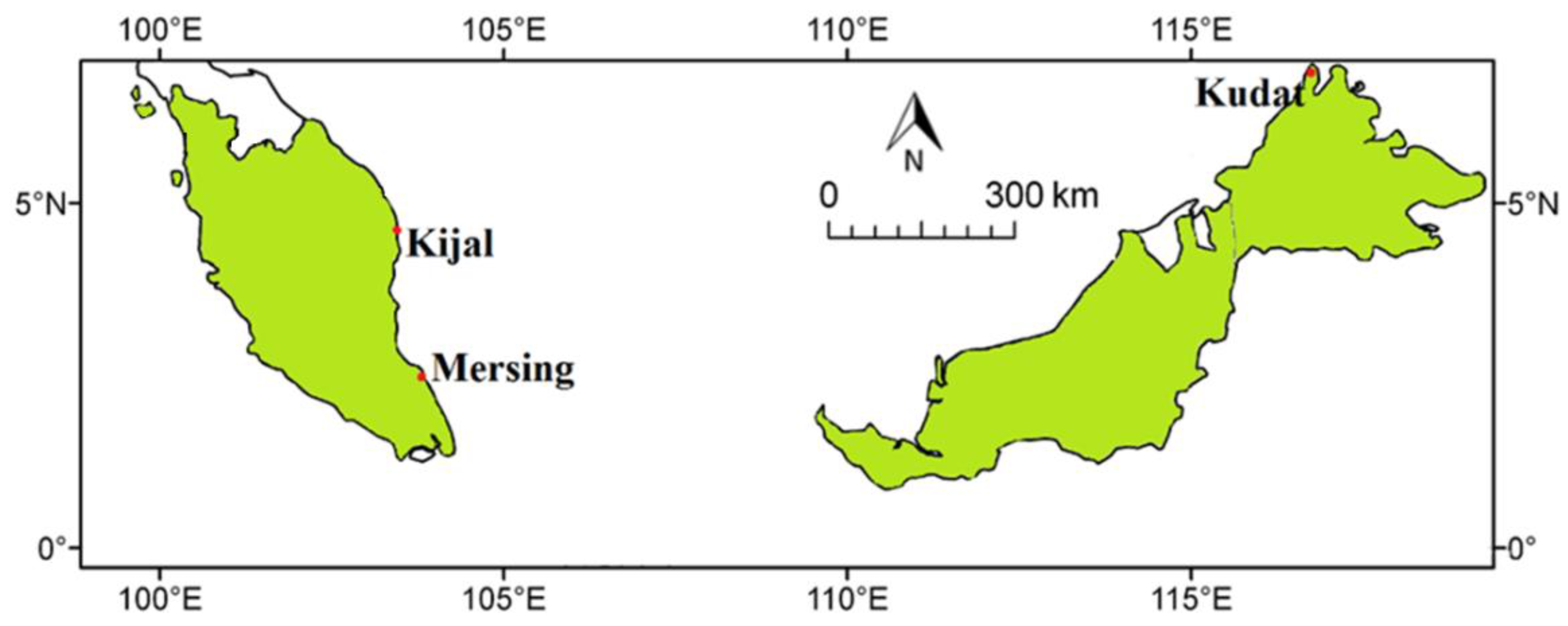
2.1. Data Description

This study used three types of wind data; (i) wind mast data that was measured at multiple heights, (ii) wind data that was measured by the Malaysia Meteorological Department (MMD) and (iii) the reanalysis wind data. The reanalysis data that was used in this study is from the extended Climate Forecast System Reanalysis (CFSRE).

The wind mast and MMD data were measured data collected using the sensors, and stored in the data logger of a wind measurement mast situated at three locations, namely Kudat in Sabah; Mersing in Johor; and Kijal in Terengganu, as shown in Figure 1 and

Table 1. The sites of the measured wind mast, the Malaysia Meteorological Department (MMD) and Climate Forecast System Reanalysis (CFSRE).

Data	Information	Kudat	Mersing	Kijal
Wind mast data	Coordinates	7°1′45.33″ N 116°44′47.98″ E	2°34′50.00″ N 103°48′23.60″ E	4°20′50.70″ N 103°28′34.74″ E
	Height	10 m, 70 m	10 m, 60 m	10 m, 60 m
	Power law index (PLI)	0.38	0.20	0.25
	Period	May 2014–April 2015 (12 Months) 52,560 data Recovery: 99%	January 2014–December 2014 (12 Months) 52,560 data Recovery: 99%	May 2013–April 2014 (12 Months) 52,560 data Recovery: 99%
MMD data	Coordinates	6°55′12.00″ N 116°49′48.00″ E	2°27′0.00″ N 103°49′48.00″ E	5°22′48.00″ N 103°5′60.00″ E
	Height	10 m	10 m	10 m
	Period	1 January 2006–December 2016	1 January 2006–December 2016	1 January 2006–December 2016
CFSRE data	Coordinates	7°0′0.00″ N 117°0′0.00″ E	2°30′0.00″ N 103°59′60.00″ E	4°0′0.00″ N 103°29′60.00″ E
	Height	10 m	10 m	10 m
	Period	1 January 1983–31 December 2017	1 January 1983–31 December 2017	1 January 1983–31 December 2017

. The wind mast data were measured at our temporarily installed wind measurement mast, while the MMD data was directly obtained from the Malaysian Meteorological Department.

The wind mast measurements were carried out in accordance with IEC 61400-12-1 [14]. The selection of the sites was based on the several previous studies that confirmed the potential of those sites for wind energy projects in Malaysia [15,16,17,18]. Most of the literature indicates that the east coast of peninsular Malaysia and the northern part of Sabah are the most promising sites for wind energy in the country. In addition, the site selection was also based on field inspection trips and preliminary wind resource maps. The factors which are considered in the selection of sites were: the difficulty of access, the availability of grid connection, and the wind quality. Every mast was mounted with more than one anemometer to assess the power law indexes. The mounting of these additional anemometer followed the IEC 61400-12-1 [14] as well as procedures recommended in the IEA guidelines [19]. The maximum height of the wind mast tower was different for every site, ranging from 60 m to 70 m (m.a.g.l). Higher measurement heights reduces the uncertainty of the vertical extrapolation of the wind speed. The data are checked and validated on a monthly basis to detect possible defects in time and to limit any data losses. The data losses and outliers could affect the result of the wind resource assessment [20]. The data validation methods were employed based on the methods suggested by [21,22].

The extended Climate Forecast System Reanalysis (CFSRE) is an extended version of the dataset from the first and second version of the CFSR. It was developed by the United States National Oceanic and Atmospheric Administration (NOAA), United States National Centers for Environmental Prediction (NCEP), and United States National Weather Service (NWS). The CFSR is generated based on the following factors [23]: (i) coupling of atmosphere and ocean during the generation of the six hour guess field; (ii) an interactive sea-ice model (for iced region); (iii) surface model; and (iv) assimilation of satellite radiances. The spatial resolution is 0.5 degrees, and the data are available from 1979 to the present. The correlation between CFSR data with the measured data is in the range 0.81–0.91 [24]. A similar range of correlations from several studies on the CFSR data for different countries is summarized in [25]. The value is quite acceptable and shows the suitability for wind data prediction or climate analysis. In addition, higher spatial and temporal resolutions of the CFSR datasets allow better representation of the local wind climate by the high levels of correlation with the data records obtained from the anemometers installed on local masts [26]. To start the study of climate, especially in relation to the impact of ENSO, at least around 35 years of wind data is needed [27]. Therefore, in this paper, 35 years of data from 1983 to 2017 were utilized.

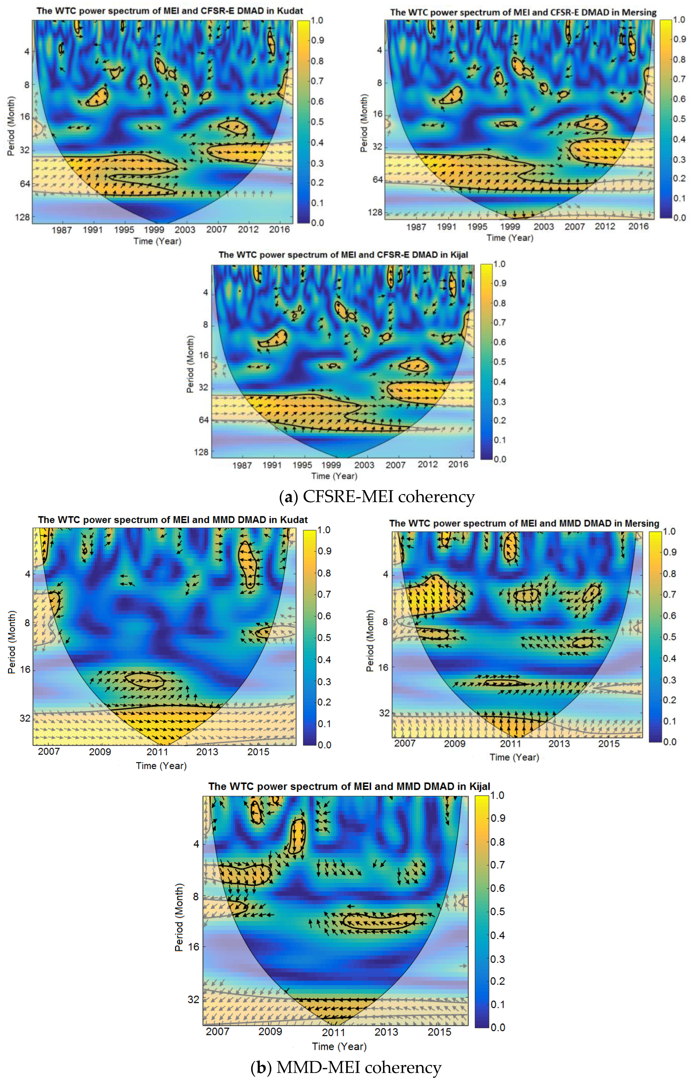
2.2. Wavelet Coherence

Many signals, such as atmospheric parameters, are irregular and non-stationary. Compared to Fourier transform, Wavelet transform was chosen because of its ability to achieve a variable resolution in one domain (either frequency or time) and multi-resolution in the other domain [28]. The spectral behaviour of a time series also can be studied using the Wavelet transform. Hence, to investigate the relationships of wind speed and MEI (ENSO index), the Wavelet Coherence (WTC) is proposed. The equation for WTC is as follows [29]:

$$R_n^2(s)=\frac{{\left|S(s^{-1}{W}_n^{XY}(s))\right|}^2}{S\left(s^{-1}{\left|W_n^X\right|}^2\right)S\left(s^{-1}{\left|W_n^Y\right|}^2\right)}$$

(1)

where S is the smoothing operator which is essential in coherence analysis. The smoothing operator is given by [29]:

$$S(W)=S_{\mathrm{scale}}(S_{\mathrm{time}}(W(s)))$$

(2)

where the smoothing operator along the wavelet scale is denoted as S_scale and the smoothing operator in time is denoted as S_time.

The smoothing operators are designed so that they have the same footprint as the wavelet used. The suitable S_scale and S_time for Morlet wavelet are respectively given by:

$${S_{scale}(W)|}_n={\left(W_n(s)·c_1\Pi (0.6s)\right)|}_n$$

(3)

$${S_{time}(W)|}_s={\left(W_n(s)·c_2{e}^{\frac{-n^2}{2s^2}}\right)|}_s$$

(4)

where П is the rectangular function and, c₁ and c₂ are the normalization constant. The factor 0.6 is an empirically determined scale decorrelation length for the Morlet wavelet [30]. c₁ and c₂ are determined numerically after the computation of the two convolutions (the filters c₁П(0.6s) and $c_2{e}^{-n^2/2s^2}$ must have unit weight).

The evaluation of the phase difference ${\varphi }_n^{XY}$ is conducted to determine the delay between two time series (wind speed and MEI data) at some specific time and scale [30]:

$${\varphi }_n^{XY}(s)={\tan }^{-1}\left(\frac{\mathsf{\Im }\left(S\left(s^{-}{W}_n^{XY}(s)\right)\right)}{\mathsf{\Re }\left(S\left(s^{-}{W}_n^{XY}(s)\right)\right)}\right)$$

(5)

where $\mathsf{\Re }\left(S\left(s^{-}{W}_n^{XY}(s)\right)\right)$ and $\mathsf{\Im }\left(S\left(s^{-}{W}_n^{XY}(s)\right)\right)$ are the real and the imaginary parts of the smoothed cross wavelet transform, respectively. ${\varphi }_n^{XY}(s)$ is not defined when $\mathsf{\Im }\left(S\left(s^{-}{W}_n^{XY}(s)\right)\right)$ is equal to zero.

2.3. Vertical Extrapolation

The wind data should be vertically predicted, as the hub height of the selected wind turbine is higher than the height of the measurement mast. The common method used to compute the vertical wind data is by using the power law method, which is also known as the Hellmann power law. The Hellmann power law, as expressed by [31,32], is given in the following:

$$v_2=v_1{\left(\frac{z_2}{z_1}\right)}^{\alpha }$$

(6)

in which v is the wind speed to height z, v₁ is the reference wind speed to reference height z₁, v₂ is the desired wind speed to desired height z₂ and α is the power law index (PLI).

2.4. Energy Production

A Goldwind wind turbine (WTG) with capacity of 1.5 MW was selected for energy analysis as it is classified as a class III wind turbine which is suitable for application in low wind speed regions. The cut-in and rated wind speed for the wind turbine is 3.0 m/s and 13 m/s, respectively. The hub height for both wind turbines is 70 m from ground level. As the selected wind turbines in this study are the pitch-regulated type, thus, the power and the energy produced by WTG were calculated by using the following equations [3]:

Power:

$$p{(v)}_{pitch}={\mathrm{P}}_{\mathrm{r}}\times \{\begin{array}{c}\begin{array}{l}0\\ \end{array}\\ {\left({\displaystyle \sum _{i=0}^n{a}_i{v}^i}\right)}_{asc}\\ \begin{array}{l}\\ 1\end{array}\end{array}\begin{array}{c}v<v_c\mathrm{or}v>v_f\\ \\ \\ \begin{array}{l}{v}_c\le v\le v_r\\ \\ v_r\le v\le v_f\end{array}\end{array}$$

(7)

Energy:

$$AE{P}_{pitch}={\mathrm{P}}_r{\displaystyle \underset{V_c}{\overset{V_r}{\int }}\left({\displaystyle \sum _{i=0}^n{a}_i{v}^i}\right)f(v)dv}+{\mathrm{P}}_r{\displaystyle \underset{V_r}{\overset{V_f}{\int }}f(v)dv}$$

(8)

where P_r is the wind turbine rated power, v_c is the cut-in wind speed, v_r is the rated wind speed, v_f is the cut-out wind speed, ${\displaystyle \sum _{i=0}^n{a}_i{v}^i}$ is the fifth order polynomial model, and f(v) is the wind speed distribution.

2.5. Accuracy Metrics

The study used three types of accuracy metric to look at the performance of every derived model and artificial data. The metrics include the coefficient of determination, the root mean square error, and the mean absolute error.

2.5.1. The Coefficient of Determination

The coefficient of determination, r, is a formula used in interpreting the proportion of variability in the data set that is taken into account by the selected statistical model. r gives some information about the goodness of fit of the chosen model. A higher r represents a better fit using the theoretical or empirical function, and the highest value is 1 [33]. The equation of r is presented as the following:

$$r=1-\frac{{\displaystyle \sum _{i=1}^n{\left(v_{a,i}-v_{b,i}\right)}^2}}{{\displaystyle \sum _{i=1}^n{\left(v_{a,i}-\overline{v}\right)}^2}}$$

(9)

where, $v_{a,i}$ is the observed data at specific period, i, $v_{b,i}$ is the artificial data, $\overline{v}$ is the mean value of $v_i$, and n is the number of all observed wind data.

2.5.2. The Root Mean Square Error

The root mean square error (RMSE) gives the deviation between the artificial and the measured values. Usually, the RMSE is better at revealing model performance differences [34]. This method is widely applied to determine the accuracy, including the studies done by [35,36]. A low RMSE indicates a successful prediction, where the RMSE should be as close to zero as possible, and it is expressed as the following:

$$\mathrm{RMSE}={\left[\frac{1}{N}{\displaystyle \sum _{i=1}^N{\left(v_{b,i}-v_{a,i}\right)}^2}\right]}^{\frac{1}{2}}$$

(10)

where, v_b,i is the artificial value and v_a,i is the observed data.

2.5.3. Mean Absolute Error

Mean absolute error (MAE) is the average over the verification sample of the absolute values of the differences between forecasts and the corresponding observations. It measures the accuracy of continuous variables. The MAE is a linear score, which means that all the individual differences are weighted equally in the average [37]. The equation is given as follows:

$$\mathrm{MAE}=\frac{1}{N}{\displaystyle \sum _{i=1}^N\left|v_{b,i}-v_{a,i}\right|}$$

(11)

3. Results and Discussion

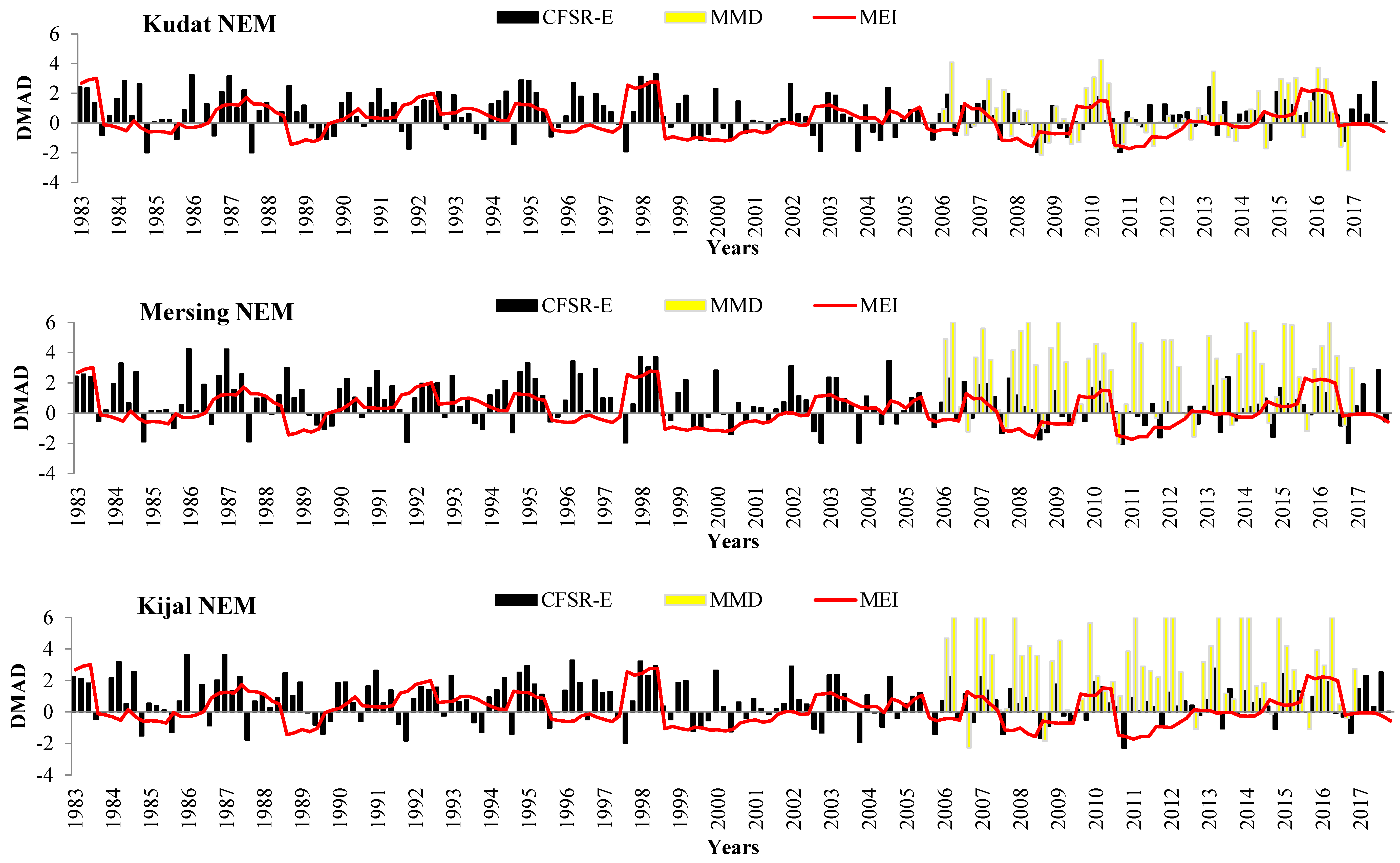
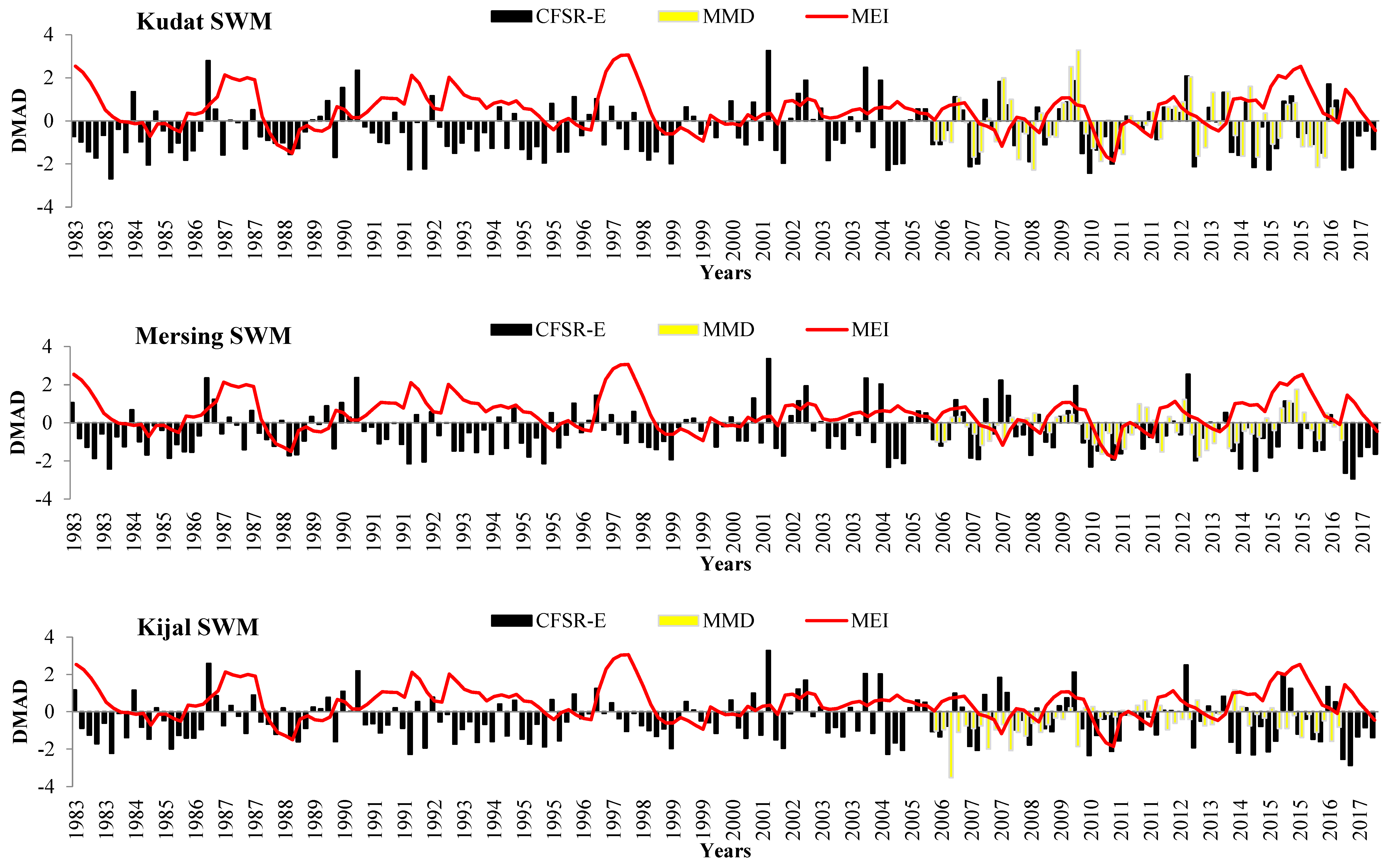
3.1. The Variability of CFSRE and MMD Data

The variability of both CFSRE and MMD in conjunction with MEI index analysis during the Southwest monsoon (SWM) and Northeast monsoon (NEM) were assessed using the dimensionless median absolute deviation (DMAD) and Wavelet coherency analysis. The SWM, also known as the dry season occurred from May to September, while the NEM (wet season) occurred from November to March. During the NEM season (Figure 2), both CFSRE and MMD for all sites show an increment in wind speed from their median level, while a decrement occurred during the SWM season (Figure 3). Similar findings regarding the variability of wind speed during both monsoons in Malaysia was also reported by [2,4,38,39]. Usually, higher precipitation with strong wind speed occurs during the NEM season compared to the SWM. In addition, the precipitation and wind strength would be reduced by the existence of El Niño and increased with La Niña.

The strength of an ENSO event based on the MEI index is identified as per the classification in [40]. El Niño strength is classified as Very Strong El Niño (VSE), Strong El Niño (SE), Moderate El Niño (ME) and Weak El Niño (WE). La Niña strengths are Strong La Niña (SL), Moderate La Niña (ML) and Weak La Niña (WL). During a SE, the wind speed is usually less than the normal range, but it was noticed that during a VSE, all sites experienced mostly higher wind speeds. It is important to mention that as each ENSO event has unique lineaments in terms of specific pattern changes, timing and intensity, the ENSO impacts on wind speed are always different for each event.

In order to study the relationship between the wind speed and ENSO, the Wavelet coherency is evaluated here for the MMD DMAD, CFSRE DMAD and MEI data series (see Figure 4). The values derived using the WTC vary between 0 and 1. The closer the WTC is to 1 the more coherencies there is between the time series. The horizontal axis is the time scale (in years) and the vertical axis is the period (1/frequency). The cone-shaped line is the cone of influence, which indicates the region affected by the edge effect. The 5% significance level against red noise is shown as a thick contour. The coherency ranges were defined based on a color code from dark blue (low coherency, close to zero) to yellow (high coherency, close to one). Moreover, black arrows indicate the phase difference between two sets of time series data which were only plotted for coherence equal or more than 0.5. The arrow pointing to the right mean that the variables are in phase. The arrow pointing to the right is in-phase, and is anti-phase when pointing to the left. The wind speed leading the ENSO index by 90° points straight down, while it is lagging when it points straight up.

For CFSRE-MEI (1983–2017), the distribution of significant coherence is quite similar for all sites and occurred in two periods from 4–16 days and 32–64 days. High and significant coherence values occurred around the period of 32–64 days and are persistent across the spectrum from 1983–2017. In this period band, the two time series are approximately in-phase as represented by arrows pointing to the right, which suggests that the wind speed was positively correlated with the MEI index. The phase difference between CFSRE and MEI shows a clear seasonal variability. For MMD-MEI (2006–2016), the distribution of significant coherence is different for different sites. In Kudat, significant coherence occurred at period 2–6 (2014–2015) and period 6–10 (2006–2007). In Mersing, significant coherence occurred at period 1–3 (2011–2012) and period 4–8 2006–2010). In Kijal, significant coherence occurred at period 1–5 (2009–2010) and period 6–10 (2007–2012). The most significant coherence values for CFSRE-MEI (all sites) occur around 32–64 months, while for MMD-MEI they occur after 31 months. The arrows show the strong in-phase relationship for CFSRE-MEI, which suggests the positive correlation of the two series. However, for MMD-MEI, the arrows show a strong in-phase relationship only at Kudat, while in Kijal they are anti-phase. In addition, the arrows in Mersing are anti-phase (2006–2012) and in-phase (2013–2016).

3.2. The Wind Speed Prediction

The measured wind mast data only covers a short period of around one to three years. Therefore, to study the long-term wind energy potential, data prediction should be conducted. The data prediction adopted sectoral regression by using a Measure-Correlate Predict (MCP) approach. MCP is widely used in establishing long-term wind statistics using limited wind data from the measured site and the long-term wind data from nearby sites. The concurrent measured and nearby long-term wind data (CFSRE and MMD) were utilized to generate the transfer function. Based on the generic transfer function, the predicted data can be generated using the nearby long-term data as a reference. There are many types of MCP approaches, including the linear regression method [41,42] and matrix method [43,44]. Despite the various available MCP methods, linear regression is the most widely used method in the wind industry, presumably due to its straight forwardness and effectiveness [25]. Therefore, the linear sectoral regression was used to predict the long-term data. By using this regression, the concurrent data were grouped into different 30° sectors based on the wind direction. The available data on the sector was correlated and used to derive the linear transfer function. The residual model is also included, where the zero mean Gaussian distribution model [45], e ~ N (0,s), was adopted. The neglect of residual in linear regression prediction can lead to 10% of erroneously as mentioned in [46]. The parameters of linear regression were estimated by a least squares algorithm.

Table 2. The correlation coefficient and accuracy analysis of concurrent reanalysis and predicted data with measured wind mast data.

Site	Metrics	CFSRE	MMD	MCP-MMD	MCP-CFSRE
Kudat	r	0.4532	0.2538	0.1879	0.4174
	MAE	1.0518	1.1389	1.1664	1.0899
	RMSE	2.0815	1.8510	2.0767	1.6676
Mersing	r	0.4610	0.3861	0.3788	0.4303
	MAE	1.2748	1.3233	1.3232	1.2886
	RMSE	1.9503	1.7871	1.9046	1.8219
Kijal	r	0.5481	0.5161	0.4445	0.4599
	MAE	1.0019	1.0410	1.0788	1.0729
	RMSE	1.8376	1.3759	1.6182	1.5275

shows the r, MAE and RMSE results for concurrent CFSRE and MMD data with measured wind mast data. It is shown that the MCP with CFSRE is more accurate and worked well with the measured wind mast data. The results may be influenced by geographical factors as the CFSRE data point was situated near to the site where the mast tower was installed, while the MMD station was located far from the mast site. The correlation coefficient for MCP-CFSRE is in between 0.4174–0.4599, indicating a close to moderately strong relationship between the variables [47]. The wind RMSE and MAE of MCP-CFSRE also shows better results compared to MCP-MMD. The MAE is the average value of the residuals. The Durbin-Watson (DW) statistic tests the residuals to determine if there is any significant correlation. Since the p-value is less than 0.05, there is an indication of possible serial correlation at the 95.0% confidence level.

The Weibull distribution function is used to identify the precision of the range and distribution of the wind speed for all concurrent data. The scale parameter is used to measure the wind speed characteristics of the distribution, and it is proportional to the mean wind speed. The shape parameter, k, specifies the shape of a distribution. A small value of k signifies variable winds, while constant winds are characterized by a larger k. The value of shape parameter was equal to or more than 2.00, indicating that the wind speed data tended to be uniformly distributed over a relative range of wind speeds. The higher the value of the wind speed, the more the Weibull curve will skew to the right. This skewed curve means there is more potential for wind power and energy density.

Table 3. The mean wind speed and Weibull parameters of all data.

Site	Data	Signal	Mean	Weibull Mean	Weibull Scale, c	Weibull Shape, k
Kudat	CFSRE Concurrent	Mean wind speed, m/s	3.76	3.81	4.30	2.12
		Wind direction, Degrees	106.20	-	-	-
	MMD Concurrent	Mean wind speed, m/s	2.52	2.72	3.07	2.07
		Wind direction, Degrees	156.8	-	-	-
	Mast	Mean wind speed, m/s	2.82	2.85	3.21	1.84
		Wind direction, Degrees	171.10	-	-	-
	MCP-CFSRE Concurrent	Mean wind speed, m/s	2.77	2.85	3.22	2.05
		Wind direction, Degrees	175.20	-	-	-
	MCP-MMD Concurrent	Mean wind speed, m/s	2.93	3.03	3.43	1.99
		Wind direction, Degrees	198.00	-	-	-
Mersing	CFSRE	Mean wind speed, m/s	3.36	3.41	3.84	2.38
		Wind direction, Degrees	111.40	-	-	-
	MMD	Mean wind speed, m/s	2.83	2.97	3.36	2.28
		Wind direction, Degrees	268.40	-	-	-
	Mast	Mean wind speed, m/s	2.43	2.59	2.90	1.67
		Wind direction, Degrees	164.40	-	-	-
	MCP-CFSRE	Mean wind speed, m/s	2.45	2.60	2.92	1.75
		Wind direction, Degrees	133.30	-	-	-
	MCP-MMD	Mean wind speed, m/s	2.49	2.63	2.96	1.78
		Wind direction, Degrees	174.40	-	-	-
Kijal	CFSRE	Mean wind speed, m/s	3.36	3.40	3.83	2.19
		Wind direction, Degrees	22.8	-	-	-
	MMD	Mean wind speed, m/s	2.09	2.34	2.65	2.14
		Wind direction, Degrees	149.9	-	-	-
	Mast	Mean wind speed, m/s	2.31	2.47	2.77	1.76
		Wind direction, Degrees	20.2	-	-	-
	MCP-CFSRE	Mean wind speed, m/s	2.26	2.37	2.67	1.82
		Wind direction, Degrees	330.00	-	-	-
	MCP-MMD	Mean wind speed, m/s	2.34	2.44	2.74	1.71
		Wind direction, Degrees	329.6	-	-	-

presents the concurrent period of mean wind speed and Weibull parameters for all data. It shows that the CFSRE has a higher value compared to the measured mast and MMD data. However, the predicted data of MCP-CFSRE and MCP-MMD is close to the measured mast data (see Figure 5). This proves that the sectoral regression method is a robust method for long-term wind prediction.

3.3. Long Term Wind Energy Potential

Based on the MCP-CFSRE and MCP-MMD, the gross long-term monthly capacity factor of the Goldwind 1.5 MW WTG was computed and plotted. The monthly capacity factor (CF) was computed based on different monsoon seasons, NEM and SWM, and plotted on the same graph. The CF for MCP-CFSRE is computed for a 35-year period as the reference data for CFSRE is available from 1983 to 2017. For MCP-MMD, the period is 10 years, from 2006 to 2016. The CF refers to the ratio of estimated and nominal annual energy production. The energy production at specific periods (monthly or seasons) for the selected Goldwind 1.5 MW wind turbine was simulated at selected sites where the wind measurement masts were installed. After the value of annual energy production (AEP) had been determined, the CF was then computed as a percentage. The best CF that is feasible and promising for an energy project is 20% and above. In fact, a CF of 20% has been determined as the best CF to attain profitability of wind energy project [48].

The level of monthly averaged CF for both MCP-CFSRE and MCP-MMD during the NEM and SWM seasons show the same trend (See Figure 6). The CF during the NEM is higher compared to the SWM for Kijal and Mersing. In Kijal the average CF is 10.66% during the NEM and 5.19% during the SWM, while the average CF in Mersing during the NEM and SWM are 21.32% and 3.71%, respectively. However, in Kudat, where the monthly averaged CF is almost the same for both the SWM and NEM season. In addition, the monsoonal averaged CF at Kudat during the SWM (36.42%) is slightly higher compared to the NEM (24.61%). This can be explained by their geographical location. Kijal and Mersing are located on the east coast of peninsular Malaysia. Therefore, during the SWM, the southwesterly wind is blocked by the Titiwangsa range, which reduces the impact of the monsoon. However, based on a report by [49], during the SWM tropical storms exist in the South China Sea and Pacific Ocean, thus, there are tail-effects on the wind strength in the northern part of Sabah. This will increase the energy production of wind turbines during this period (see

Table 4. The average of monthly CF during both monsoon seasons throughout the years of the reference data period.

Data	Composition	Kudat	Mersing	Kijal
MCP-CFSRE (35-years)	Average CF (%); NEM + SWM	30.56	11.49	7.24
	Average CF (%); NEM only	24.61	21.32	10.66
	Average CF (%); SWM only	36.42	3.71	5.19
MCP-MMD (10 years)	Average CF (%); NEM + SWM	30.25	11.75	11.93
	Average CF (%); NEM only	23.57	18.14	16.20
	Average CF (%); SWM only	35.79	7.92	8.73

).

4. Conclusions and Recommendation

In this study, the long-term wind energy variability of selected sites in Malaysia was investigated. The data that was utilized in the analysis are: (i) one-year data that newly measured the three selected sites, (ii) ten years of data obtained from meteorological data, and (iii) 35 years extended CFSR reanalysis wind data. The findings of this paper are as follows:

• The influences of ENSO on the wind speed pattern of selected sites were assessed using the DMAD method during the Southwest monsoon (SWM) and Northeast monsoon (NEM). During the NEM season, both CFSRE and MMD for all sites show an increment in wind speed from their median levels, while a decrement occurred during the SWM season.
• The wavelet coherency analysis is useful to study the interaction and the relative phase between two time series. The relationships between wind speed and MEI time series data showed the strongest correlation at around the 32–64 months period band for CFSRE-MEI and above 31 months for MMD-MEI coherency.
• Long-term wind energy production was determined by averaging the 35 years (MCP-CFSRE) and 10 years (MCP-MMD) of computed capacity factor (CF). The averaged CF during the NEM was higher compared to the SWM for Kijal and Mersing. In Kijal the average CF is 10.66% during the NEM and 5.19% during the SWM, while the average CF in Mersing during NEM and SWM are 21.32% and 3.71% respectively. However, the result is different for Kudat where the monthly CF is almost the same for both the SWM and NEM season. The average CF at Kudat during the SWM (36.42%) is slightly higher compared to the NEM (24.61%).
• The ENSO (MEI index) has an influence on the variability of wind speed (CFSRE and MMD) in Malaysia, which also directly affects the projected energy production.

References

1. Albani, A.; Ibrahim, M.Z. An assessment of wind energy potential for selected sites in Malaysia using feed-in tariff criteria. Wind Eng. 2014, 38. [Google Scholar] [CrossRef]
2. Ibrahim, M.Z.; Albani, A. The potential of wind energy in Malaysian renewable energy policy: Case study in kudat, sabah. Energy Environ. 2014, 25. [Google Scholar] [CrossRef]
3. Albani, A.; Ibrahim, M.Z. Wind Energy Potential and Power Law Indexes Assessment for Selected Near-Coastal Sites in Malaysia. Energies 2017, 10, 307. [Google Scholar] [CrossRef]
4. Muzathik, A.M.; Nik Wan, W.B.; Ibrahim, M.Z.; Samo, K.B. Wind resource investigation of Terengganu in the west Malaysia. Wind Eng. 2009, 33, 389–402. [Google Scholar] [CrossRef]
5. Landberg, L.; Myllerup, L.; Rathmann, O.; Petersen, E.L.; Jørgensen, B.H.; Badger, J.; Mortensen, N.G. Wind resource estimation—An overview. Wind Energy 2003, 6, 261–271. [Google Scholar] [CrossRef]
6. Weekes, S.M.; Tomlin, A.S.; Vosper, S.B.; Skea, A.K.; Gallani, M.L.; Standen, J.J. Long-term wind resource assessment for small and medium-scale turbines using operational forecast data and measure-correlate-predict. Renew. Energy 2015, 81, 760–769. [Google Scholar] [CrossRef]
7. Bueno, C.; Carta, J.A. Wind powered pumped hydro storage systems, a means of increasing the penetration of renewable energy in the Canary Islands. Renew. Sustain. Energy Rev. 2006, 10, 312–340. [Google Scholar] [CrossRef]
8. Zelle, H.; Appeldoorn, G.; Burgers, G.; van Oldenborgh, G.J. The Relationship between Sea Surface Temperature and Thermocline Depth in the Eastern Equatorial Pacific. J. Phys. Oceanogr. 2004, 34, 643–655. [Google Scholar] [CrossRef] [Green Version]
9. Agilan, V.; Umamahesh, N.V. Detection and attribution of non-stationarity in intensity and frequency of daily and 4-h extreme rainfall of Hyderabad, India. J. Hydrol. 2015, 530, 677–697. [Google Scholar] [CrossRef]
10. Wolter, K.; Timlin, M.S. Measuring the strength of ENSO events: How does 1997/98 rank? Weather 1998, 53, 315–324. [Google Scholar] [CrossRef]
11. Mohammadi, K.; Goudarzi, N. Study of inter-correlations of solar radiation, wind speed and precipitation under the influence of El Niño Southern Oscillation (ENSO) in California. Renew. Energy 2018, 120, 190–200. [Google Scholar] [CrossRef]
12. Watts, D.; Durán, P.; Flores, Y. How does El Niño Southern Oscillation impact the wind resource in Chile? A techno-economical assessment of the influence of El Niño and La Niña on the wind power. Renew. Energy 2017, 103, 128–142. [Google Scholar] [CrossRef]
13. Hamlington, B.D.; Hamlington, P.E.; Collins, S.G.; Alexander, S.R.; Kim, K.Y. Effects of climate oscillations on wind resource variability in the United States. Geophys. Res. Lett. 2015, 42, 145–152. [Google Scholar] [CrossRef] [Green Version]
14. IEC. IEC61400-12-1 Wind Turbines-Part 12-1: Power Performance Measurement of Electricity Producing Wind Turbines, 1st ed.; IEC: Geneva, Switzerland, 2005. [Google Scholar]
15. Ibrahim, M.Z.; Yong, K.H.; Ismail, M.; Albani, A.; Muzathik, A.M. Wind characteristics and gis-based spatial wind mapping study in Malaysia. J. Sustain. Sci. Manag. 2014, 9, 1–20. [Google Scholar]
16. Ibrahim, M.Z.; Yong, K.H.; Ismail, M.; Albani, A. Spatial Analysis of Wind Potential for Malaysia. Int. J. Renew. Energy Res. 2015, 5, 202–209. [Google Scholar]
17. Ibrahim, M.Z.; Albani, A. Wind turbine rank method for a wind park scenario. World J. Eng. 2016, 13, 500–508. [Google Scholar] [CrossRef]
18. Albani, A.; Ibrahim, M.; Yong, K. The feasibility study of offshore wind energy potential in Kijal, Malaysia: The new alternative energy source exploration in Malaysia. Energy Explor. Exploit. 2014, 2. [Google Scholar] [CrossRef]
19. IEA. IEA Recommendation 11: Wind Speed Measurement and Use of Cup Anemometry; IEA: Paris, France, 1999. [Google Scholar]
20. Wettayaprasit, W.; Laosen, N.; Chevakidagarn, S. Data filtering technique for neural network forecasting. In Proceedings of the 7th WSEAS International Conference on Simulation, Modelling and Optimization, Beijing, China, 15–17 September 2007. [Google Scholar]
21. Mueller, P.K.; Watson, J.G. Eastern Regional Air Quality Measurements; Environmental Research and Technology, Inc.: Concord, MA, USA, 1982; Volume 1, Available online: https://www.osti.gov/biblio/6730513-eastern-regional-air-quality-measurements-volume-final-report (accessed on 1 December 2017).
22. Watson, J.G.; Lioy, P.J.; Mueller, P.K. The measurement process: Precision, accuracy, and validity. In Air Sampling Instruments for Evaluation of Atmospheric Contaminants, 7th ed.; Hering, S.V., Ed.; American Conference of Governmental Industrial Hygienists: Cincinnati, OH, USA, 1989; pp. 51–57. [Google Scholar]
23. NCAR. The Climate Data Guide: Climate Forecast System Reanalysis (CFSR). Natl Cent Atmos Res Staff n.d. Available online: https://climatedataguide.ucar.edu/climate-data/climate-forecast-system-reanalysis-cfsr (accessed on 3 October 2016).
24. Sharp, E.; Dodds, P.; Barrett, M.; Spataru, C. Evaluating the accuracy of CFSR reanalysis hourly wind speed forecasts for the UK, using in situ measurements and geographical information. Renew. Energy 2015, 77, 527–538. [Google Scholar] [CrossRef]
25. Carta, J.A.; Velazquez, S.; Cabrera, P. A review of measure-correlate-predict (MCP) methods used to estimate long-term wind characteristics at a target site. Renew. Sustain. Energy Rev. 2013, 27, 362–400. [Google Scholar] [CrossRef]
26. Liléo, S.; Petrik, O. Investigation on the use of NCEP/NCAR, MERRA and NCEP/CFSR reanalysis data in wind resource analysis. In Proceedings of the European Wind Energy Conference and Exhibition, Brussels, Belgium, 14–17 March 2011. [Google Scholar]
27. Yeo, S.R.; Kim, K.Y. Global warming, low-frequency variability, and biennial oscillation: An attempt to understand the physical mechanisms driving major ENSO events. Clim. Dyn. 2014, 43, 771–786. [Google Scholar] [CrossRef]
28. Victor, C.C.; Ling, H. Time-Frequency Transforms for Radar Imaging and Signal Analysis; Artech House: Boston, MA, USA; London, UK, 2002. [Google Scholar]
29. Chellali, F.; Khellaf, A.; Belouchrani, A. Wavelet spectral analysis of the temperature and wind speed data at Adrar, Algeria. Renew. Energy 2010, 35, 1214–1219. [Google Scholar] [CrossRef]
30. Torrence, C.; Compo, G.P. A Practical Guide to Wavelet Analysis. Bull. Am. Meteorol. Soc. 1998, 79, 61–78. [Google Scholar] [CrossRef] [Green Version]
31. Zhang, J.; Draxl, C.; Hopson, T.; Monache, L.D.; Vanvyve, E.; Hodge, B.M. Comparison of numerical weather prediction based deterministic and probabilistic wind resource assessment methods. Appl. Energy 2015, 156, 528–541. [Google Scholar] [CrossRef] [Green Version]
32. Jung, S.; Arda Vanli, O.; Kwon, S.-D. Wind energy potential assessment considering the uncertainties due to limited data. Appl. Energy 2013, 102, 1492–1503. [Google Scholar] [CrossRef]
33. Kidmo, D.K.; Doka, S.Y.; Danwe, R.; Djongyang, N. Performance Analysis of Weibull Methods for Estimation of Wind Speed Distributions in the Adamaoua Region of Cameroon. Int. J. Basic Appl. Sci. 2014, 3, 298–306. [Google Scholar] [CrossRef]
34. Chai, T.; Draxler, R.R. Root mean square error (RMSE) or mean absolute error (MAE)?-Arguments against avoiding RMSE in the literature. Geosci. Model Dev. 2014, 7, 1247–1250. [Google Scholar] [CrossRef]
35. Azad, A.K.; Rasul, M.G.; Yusaf, T. Statistical Diagnosis of the Best Weibull Methods for Wind Power Assessment for Agricultural Applications. Energies 2014, 7, 3056–3085. [Google Scholar] [CrossRef] [Green Version]
36. Costa Rocha, P.A.; Coelho de Sousa, R.; Freitas de Andrade, C.; Vieira da Silva, M. Comparison of Seven Numerical Methods for Determining Weibull Parameters for Wind Energy Generation in the Northeast Region of Brazil. Appl. Energy 2012, 89, 395–400. [Google Scholar] [CrossRef]
37. Willmott, C.J.; Matsuura, K. Advantages of the mean absolute error (MAE) over the root mean square error (RMSE) in assessing average model performance. Clim. Res. 2005, 30, 79–82. [Google Scholar] [CrossRef] [Green Version]
38. Albani, A. Statistical Analysis of Wind Power Density Based on the Weibull and Rayleigh Models of Selected Site in Malaysia. Pak. J. Stat. Oper. Res. 2013, 9, 393–406. [Google Scholar] [CrossRef]
39. Albani, A.; Ibrahim, M.Z.; Taib, C.M.I.C.; Azlina, A.A. The optimal generation cost-based tariff rates for onshore wind energy in Malaysia. Energies 2017, 10, 1114. [Google Scholar] [CrossRef]
40. Mazzarella, A.; Giuliacci, A. Adriano Mazzarella The El Niño events their classification. Ann. Geophys. 2009, 52, 517–522. [Google Scholar]
41. Rogers, A.L.; Rogers, J.W.; Manwell, J.F. Comparison of the performance of four measure-correlate-predict algorithms. J. Wind Eng. Ind. Aerodyn. 2005, 93, 243–264. [Google Scholar] [CrossRef]
42. Derrick, A. Development of the measure-correlate-predict strategy for site assessment. In Proceedings of the 14th British Wind Energy Association Annual Conference, Nottingham, UK, 25–27 March 1992; pp. 259–265. [Google Scholar]
43. Woods, J.C.; Watson, S.J. A new matrix method of predicting long-term wind roses with MCP. J. Wind Eng. Ind. Aerodyn. 1997, 66, 85–94. [Google Scholar] [CrossRef]
44. Mortimer, A. A new correlation/prediction method for potential wind farm sites. In Proceedings of the Bwea Wind Energy Conference, Sterling, UK, 15–17 June 1994; p. 1994. [Google Scholar]
45. Ross, S. Introduction to Probability and Statistics for Engineers and Scientists; John Wiley & Sons: Hoboken, NJ, USA, 1987. [Google Scholar]
46. Thøgersen, M.L.; Nielsen, P.; Sørensen, T.; Svenningsen, L.U. An Introduction to the MCP Facilities in WindPRO. EMD International A/S 2010. Available online: http://help.emd.dk/knowledgebase/ content/ReferenceManual/MCP.pdf (accessed on 1 January 2018).
47. Statstutor. Spearman’s Correlation n.d. Available online: http://www.statstutor.ac.uk/resources/uploaded/spearmans.pdf (accessed on 10 September 2018).
48. Wirachai, R. The Combination of Small and Megawatt Wind Machine in Wind Farm Design for Low Wind Speed Zones. In Proceedings of the Asia Pacific Economic Corporation (APEC) Seminar Best Practices of Wind Energy Development in the APEC Region, Lima, Peru, 4–5 October 2016. [Google Scholar]
49. Wang, G.; Su, J.; Ding, Y.; Chen, D. Tropical cyclone genesis over the south China sea. J. Mar. Syst. 2007, 68, 318–326. [Google Scholar] [CrossRef]
Figure 1. Map showing the selected sites.
Energies 11 02965 g001
Figure 2. The dimensionless median absolute deviation (DMAD) for CFSRE and MMD data during the Northeast monsoon (NEM) season.
Energies 11 02965 g002
Figure 3. The DMAD for CFSRE and MMD data during the Southwest monsoon (SWM) season.
Energies 11 02965 g003
Figure 4. Wavelet coherency analysis.
Energies 11 02965 g004
Figure 5. The comparison of the Weibull distribution function of wind mast data and four points of extended CFSR.
Energies 11 02965 g005
Figure 6. The long-term energy production.
Energies 11 02965 g006