Winds of Change: How Up-To-Date Forecasting Methods Could Help Change Brazilian Wind Energy Policy and Save Billions of US$

Abstract

This paper proposes a revaluation of the Brazilian wind energy policy framework and the energy auction requirements. The proposed model deals with the four major issues associated with the wind policy framework that are: long-term wind speed sampling, wind speed forecasting reliability, energy commercialization, and the wind farm profitability. Brazilian wind policy, cross-checked against other countries policies, showed to be too restrictive and outdated. This paper proposes its renewal, through the adoption of international standards by Brazilian policy-makers, reducing the wind time sampling necessary to implement wind farms. To support such a policy change, a new wind forecasting method is designed. The method is based on fuzzy time series shaped with a statistical significance approach. It can be used to forecast wind behavior, by drawing the most-likely wind energy generation intervals given a confidence degree. The proposed method is useful to evaluate a wind farm profitability and design the biding strategy in auctions.

1. Introduction

1.1. Motivation

Brazilian government aims at installing 17GW of new wind generation capacity by 2024 [1]. This represents a 10.9% expansion in the Brazilian energy matrix, and it is sufficient to power supply 18 million residences [2]. New technologies available in last energy auctions have been forcing a sharp negative goodwill in energy prices. Voltalia SA won the 2018 first Brazilian wind energy auction, offering R$96.60/MWh (US$29.82) [3], a 400% reduction and accounting for R$402.30/MWh actual Brazilian prices [4]. It means that, for each year in advance this energy is available, the Brazilians save up to R$45,524,844,000.00, or US$14.05 billion. By adopting international regulations in Brazil, it makes possible to double that number, and make the energy available two years in advance. These significant savings shed light on this paper’s investigation. Brazilian wind notices so far are based on a Brazilian self-regulation, and demand a three years time wind measurements to afford the energy generation. This aims at ensuring the energy supply, but nowadays new techniques could assure the same, saving time and attracting investments. Notwithstanding, the wind stochastic component is a challenge. Authors in [5,6] highlights the need for new and good quality forecasting methods to deal with this component in the wind energy integration to any energy matrix. Hence, this paper proposes changes in the wind energy policy and some methods to support these changes, providing a confident forecasting in a shorter time, fostering the wind energy growth in Brazil, and speeding up the reduction of energy prices.

1.2. The Literature Review

Brazilian renewable energy market growth depends strongly on the policy-makers [7]. In fact, this is a worldwide issue. Sen [8] states that renewables growth could be as fast as the policy allows, and the market is ready to shift in that direction; provided that government and entrepreneurs could reach an agreement that fits in renewables.

Other issues also block the renewables growth, such as: capital demand and operation costs, policy, site choice, external benefits, cost grid and time to grid integrations; causing economic, technical, infrastructure, market financial, regulatory and administrative barriers. A good representation of this barriers could be found in [9]. However, the key issue is that the energy policy initiatives should be shaped to break barriers that debar investments from occurring, leading to the market reliability and renewable growth [10].

Wind energy has one of the most prominent growing among the renewables, since its worldwide abundant and fuel free [11]. Differing from traditional sources, subdued on oil prices volatility or even renewables like hydroelectric, that is penalized by a trade-off between water for human consumption, agriculture, and energy generation. Altogether, new wind technologies bring wind energy to one of the lowest energy production prices [12]. Onshore wind energy, in particular, is cheaper than many other renewables [11].

The wind seasonality has also a beneficial complementarity behavior along hydroelectricity, making it possible to cheaply layup water in hydroelectric reservoirs when the wind plant is producing and later using this water to supply, and tackle the demand [13]. Since the country growth depends on its energy resources, the introduction of a renewable, not fossil-fuel dependent, and cheaper energy, could boost the national economy, saving billions in electricity fees. The European Wind Energy Association [11], for example, states that by 2020 the wind energy sector is expected to generates 520,000 jobs and €32 billion to the European Union (EU) economy.

The report [14] states the regulatory framework for wind energy growth in the EU member states, highlighting the challenges and also states the growth level expected till 2022. As reported, many countries are not expected to reach the stated level due to their policy bureaucracy to have the implementation approvals. That is also strengthened in [15].

Actual main barriers faced to increase the number of wind energy sites are reported in [14], and they are mainly concerned with bureaucracy, political and economic framework, transparency, and market structure. Countries outside the EU face similar issues, as reported by [16]. The policy-frameworks also remain as an employment key driver. Thus, a robust policy-framework could foster the wind industry, and a lame one disassembles it all [17].

Brazil has three main stakeholders driving its policy: the Ministry of Mining and Energy (MME), the Energy Research Company (EPE) and the National Electric Energy Agency (ANEEL). They define how much, from which kind, and when the energy is going to be hired. They also drive the auctions to hire this energy. The agents’ competition throughout the auctions defines the energy price and the amount hired. Wind farms joining these auctions must gather a row of requirements addressed by ANEEL, MME, and EPE policy-framework. Some are overly rigid, for instance, the wind sampling time. The EPE [1] draws the line in three years of anemometric measurements to be held on wind farm building candidate sites. Also there could not be a rate of missing data higher than 10%, or missing for 30 consecutive days. The ANEEL agrees with the period and the MME enhances this statement in [18], laying down that it is necessary at least three years of sampling. These samples are used to address the farm viability, evaluate how much energy it will generate, and are required as a prior condition to build the farm.

These three years lag period is a limitation that affects the wind farm profitability and even its feasibility as an investment. For instance, the Brazilian inflation rate in 2015 was 10.67% and the accumulated one in the last three years was 21.21% [19]. These high rates make harder for the entrepreneurs to wait three years to analyze its feasibility, and they could decide to invest in less bureaucratic markets.

In [20] it was pointed out IEC 61400-1, IEC 61400-12, MEASTNET and TG 6, as the most commonly used standards for performing and evaluating wind measurement and wind potential energy yields. The international standard IEC 61400 [21] lays down that it is necessary one year of wind speed sampling. That is two years less than the EPE and the MME instructions. By adopting this measurement time, the cost invested to build a Brazilian wind farm could be reduced by 15%, according to the Brazilian actual inflation rate [19]. That value could be even higher if accounting for the market competition and the final consumers. Both are benefited having this cheap energy available two years in advance. Drawing a comparison, this two years reduction in the approval time is enough time to build a complete wind farm. In [20] it was pointed out in between two and three years, for all the process to plan, project and build a mid-size wind farm.

Hence, it could be inferred that the Brazilian wind framework is less competitive than other markets adopting international standards as IEC 61400 [21], which is adopted in the USA, Germany through the version DIN EN 61400-12-1 [22], UK through BS EN 61400-12-1:2017 [23] and India [24], for instance. This statement is strengthened by the world ranking in wind power installed capacity, whose the top six countries are China, EUA, Germany, India, Spain, and the UK, respectively [25]. All, except China, adopted the IEC 61400.

The wind stochastic component casts an imprecision degree in any forecasting. That component is a real challenge to be dealt with in the wind energy integration to any electric grid [5]. These authors emphasize stronger the need for new and good quality forecasting methods. The Brazilian policy adopts long-term metering as the approach to deal with this imprecision. However, improved wind forecasting approaches can be a more effective way to overcome and represent this imprecision. Authors in [26] reinforces this statement, pointing out to an accurate wind power forecasting method as the major contribution for a reliable large-scale wind power system. In this regard, many wind forecasting methods were developed [27].

The wind forecasting schemes could be classified into deterministic approaches, statistical or hybrid. In [28] it was reviewed the most popular forecasting techniques, highlighting Artificial Neural Network (ANN), Autoregressive Integrated Moving Average (ARIMA), Support Vector Machines (SVM), Case-Based Reasoning (CBR), Fuzzy time series (FTS), Grey prediction model, Moving average and exponential smoothing (MA & ES), k-Nearest Neighbor prediction method (kNN) and Hybrid models. Each of them owns a particular advantage and disadvantage. Notwithstanding, a 100% accuracy time series forecasting may not be possible, but the forecasting accuracy and processing speed can be enhanced.

The wind characteristics cannot be described accurately, having an intrinsic imprecision and incomplete knowledge on it. Purely mathematical or statistical models do not deal well with imprecise knowledge, and therefore their accuracies are below the satisfactory levels in these cases [29]. Hence, Fuzzy Time Series (FTS) become a good candidate to resolve forecasting problems since they are based on uncertain and imprecise information pertaining time series data. They are also suitable to represent linguistic variables such as $Temp=[$low, medium, high], and thus, can represent qualitative inputs, and numeric ones at the same time. For example, a specialist advice, or a qualitative index.

Wind power predictions are commonly provided in point forecasts, which correspond to a single value for each look ahead [30]. As an advantage, this approach is easier to understand, however it is less representative, since it represents only the most-likely outcome, overlooking the most-likely outcome region. Interval forecasting, as proposed in [31], are rarer in the literature, but allows an insightful understanding of the possible forecasting area.

In short, the literature review disclosed the benefits of wind energy showing that it is cheap [4], abundant [11], and renewable [12]. It also highlighted its challenges such as the stochastic behavior [13], its energy grid integration [6], and the need for good quality forecasting methods [5]. However, the literature did not reveal any proposal to change the actual Brazilian wind policy in such a way to reduce the wind power plants implementation time. This is an unsolved issue in the current body of knowledge and that is addressed in this study. This work aims at filling this gap, bringing the wind energy benefits in a shorter time to the Brazilian market, and making it competitive worldwide.

Given the above arguments, this paper proposals for the Brazilian wind policy are: adopting international standards such that IEC 61400, which are less restrictive than Brazilian policy-makers standards, and reduce the sample time duration in wind sites to obtain building approvals. Section 2 develops this idea, proposing an improved wind forecast approach to enhance the proposed changes in the Brazilian energy policy.

1.3. The Main Contributions

The paper enhances the literature in two main aspects: proposing an improvement in the Brazilian wind energy policy-framework, and a new wind forecasting method to support this policy change. The new method is used to forecast the wind behavior and wind energy generation. It is based on Fuzzy Time Series (FTS) with a statistical processing in the universe of discourse. That makes possible to draw the pessimist, optimistic, and the most-likely forecasts with a certain degree of confidence, and also design a risk index. This is helpful in tackling the main issues regarding the energy production that are forecasting energy generation and prices.

The main contributions of this paper are listed below:

• Reducing the wind farms implementation time in Brazil:
  • fostering the wind energy growth in Brazil, adopting international standards which are less restrictive than Brazilian policy-makers standards, making it competitive worldwide;
  • drawing international attention to the Brazilian wind energy market, and bringing investments;
  • speeding up the reduction of Brazilian energy prices, more players in the grid improving competition and reducing prices;
• Introducing a reliable method to forecast the wind behavior:
  • improving the wind farm planning and helping to choose the best moment and how much energy will be sold at the energy auctions;
• Using a risk index to treat the wind samples: that allows training the model with the most likely and the most-unlikely samples, and creating a forecasting interval of confidence;
• Including a statistical analysis in the FTS universe of discourse that allows designing more representative intervals;

1.4. The Structure of the Paper

The remainder of this paper contains four sections. Section 2 proposes the method that supports the proposing changes to the current Brazilian wind energy policy and describes the applied tools. Its topics are wind power calculation, forecasting, and statistical inference. Experimental results are presented in Section 3, Section 4 discusses the work achievements, and Section 5 concludes the paper.

2. Materials and Methods

This section presents the methods designed and applied in this paper regarding energy generation, forecasting methods, and the statistical approach used.

Figure 1 contains a block diagram depicting the main sequence of steps that one has to process in order to reproduce the results of the conducted study. The proposed method was implemented in the software Matlab, 2017a release, running on Windows 10 Operational System, using a CPU Intel core i7, 8GB RAM, and the wind speed databases available on [32,33]. These databases represent the wind speed in meters per second (m/s).

This work main idea is that it is not necessary to have three years of wind measurement in a prospective wind site to have an accurate forecasting, as discussed in the last section. An up to date forecasting method could reduce significantly this time, and bring a set of benefits.

To demonstrate it, here it is proposed an adaptation of the forecast method developed by [34], represented in Figure 1, Step 3, including some improvements. This paper improves the method on Step 3, by including the optimizations of the number of clusters, and the optimization of the initial matrix of cluster center values (Step 2, based on [35,36]). In the original version, these variables are set arbitrarily. At last, it is proposed the algorithm on Step 4, that performs a statistical analysis on the forecasting, drawing the line on the risky values of energy generation and its occurrence throughout the year. Step 4 produces an insightful comprehension about the forecasting and it is the base for further decisions about the wind energy farm. The Step 3 algorithm was chosen because it beats the similar algorithm in literature, as discussed in [34].

The proposed procedure main benefit is its suitability to represent the intrinsic uncertainty of wind behavior. Both inputs and outputs uncertainties are represented. The input ones are well-represented through the fuzzy variables, that group into clusters the similar wind speed behavior, and the output ones create forecasting intervals, instead of a point forecast, to represent the wind energy stochasticity. Next, the whole procedure is detailed.

2.1. Wind Energy Generation

The wind speed and its occurrence distribution are the main variables to estimate the wind farm energy generation. Wind energy generations could be determined such as [37]:

$$O_t=\frac{1}{2}{C}_p\rho D{S}_t^3,$$

(1)

where $O_t$ is given in kW and it is the produced energy in the instant t; $Cp$ is the Power Coefficient, a measure of the wind turbine efficiency; $\rho$ is the air density constant in kg/m${}^3$, D is the wind turbine propellers area in square meters m${}^2$, and $S_t$ is the wind speed in m/s in time t.

Thereafter, energy forecasting is performed with the following FTS approach.

2.2. Fuzzy Time Series

Time series are data sets that represent the behavior of one or more variables over time, in which the variable successive observations are not independent of each other [38]. These variables have groups of behavior that repeat from time to time, and thus, could be used to estimate a similar situation in the future.

The Fuzzy Time Series concept was first proposed by Song and Chissom [39], aiming at forecasting time series using linguistic values rather than numeric values as data inputs. They proposed to partition a time series into regular intervals, creating sets of linguistic functions that define groups of behavior in each of those intervals. Then, it is determined a mathematical connection that could link a past group of behaviors to the next value in the time series. Further, the pertinence of new elements on the series are cross-checked into this structure, the new element is fitted in the respective group pattern, and then a new output is calculated.

To set the FTS fundamentals, let $\gamma \left(t\right):t=0,1,2,\cdots$, be the universe of discourse in $\mathbb{R}$ by which fuzzy sets ${\mu }_j\left(t\right)$ are defined, and t is time. Each fuzzy sets ${\mu }_j\left(t\right)$ can equally represent a numeric function or a linguistic one such as ${\mu }_1\left(t\right)=low$, ${\mu }_2\left(t\right)=medium$, .... The fuzzy sets ${\mu }_j\left(t\right)$ maps a partition of the universe of discourse, representing the variables behavior. Thereafter, $F\left(t\right)$ is called a FTS defined on $\gamma \left(t\right)$ if $F\left(t\right)$ is a collection of fuzzy sets as ${\mu }_1\left(t\right), {\mu }_2\left(t\right), {\mu }_3\left(t\right), \cdots$. If exists a fuzzy relationship $R(t$ − $1,t)$, such that $F\left(t\right)=F(t$ − $1)\circ R(t$ − $1,t)$ where ∘ is an arithmetic operator, then $F\left(t\right)$ is said to be caused by $F(t$ − $1)$. The relationship between $F\left(t\right)$ and $F(t$ − $1)$ can be denoted by $F(t$ − $1)\to F(t)$. Now assume $F(t$ − $1)=B_i$ and $F\left(t\right)=B_j$; a Fuzzy Logical Relationship (FLR) can be defined as $B_i\to B_j$, where $B_i$ is called the left-hand side (LHS) and and $B_j$ is called the right-hand side (RHS) of the fuzzy logical relationship, respectively [39]. The FTS simplest form consists of the six steps presented in Algorithm 1.

Over time, many improvements have been proposed in each of those steps proposed by [39]. The universe of discourse partition have been one of main research fields in FTS since it affects the forecast performance [40], and it is an open issue indeed [41]. Huang [42] first realized it, proposing the distribution-based and average-based approach to define the intervals size in the Cheng model [39], improving the interval fit. Many techniques were used aiming at this purpose, like the ant colony algorithm [43], imperialist algorithm [44], particle swarm [45] and genetic algorithms [46]. A further approach proposes clustering techniques in the universe of discourse partition, such as fuzzy c-means [47], Gath-Geva cluster [48] and granular information [49]. Some works developed a cluster approach directly in data history fuzzification, dismissing the creation of intervals in the universe of discourse [50,51]. The last addressed the clustering approach dismissing intervals in the universe of discourse as a better approach, rather than trying to find the best partition for the universe of discourse [34].

Algorithm 1: Fuzzy Time Series [39]

Thus, regarding the universe of discourse partition, this work implemented a clustering approach. The procedure consists of splitting the input variables into a set of clusters. The clusters are chunks of data that represents a characteristic behavior of the inputs, and it substitutes the universe of discourse partition of the FTS. Further, the weighted linear contribution of each cluster is used to map the output. This linear combination behaves as a FLR. As improvements, a subtractive cluster method is used to define the number of clusters, and do the automatic tuning of the cluster centers. The number of clusters is validated with Bezdek index.

This paper proposes a procedure that could be split into three stages: i.data processing with tuning parameters; ii.training; iii.testing.

Data processing stage implements a subtractive clustering (SC) method [52] to calculate the c number of clusters and each most likely center values $\overrightarrow{v_i}$ for each input set of data $X_{r\times N}$. Where r is the number of inputs, and N the number of observations. The matrix $V_{r\times c}={[v_1,v_2,\cdots ,v_i,\cdots ,v_c]}_r$ stores the vector of cluster prototypes center of the data set r. There is a set of c centers for each input variable $X_r$. SC algorithm is a single-pass method for estimating the number of clusters used by the FCM, as well as determining the initial centers in near-optimal values, helping the FCM convergence.

Each point $x_N$ in the row r of $X_{r\times N}$ is considered as a potential cluster center of the r input [35]. The potential $\Psi$ of data point’s $x_N$ is cross-checked with the $x_i$ other possible points and is defined as [35]

$${\Psi }_N=\sum _{i=1}^N{e}^{\frac{-4x_N-x_i^2}{l_a^2}},$$

(2)

where $l_a$ and $l_b$ are th cluster radius in data space and the cluster radius penalty, respectively. Then, let $x_1$ and ${\Psi }_1$ be the first cluster center and its respective potential. The potential is revised for each data point by using [35]:

$${\Psi }_N={\Psi }_N-{\Psi }_1{e}^{\frac{-4x_N-x_1^2}{l_b^2}}.$$

(3)

$x_1$ then becomes $v_1$, the first cluster center of the vector $\overrightarrow{v_i}$. An amount of potential is subtracted from each data point as a function of its distance from the first cluster center. The data near the first cluster center will have greatly reduced potential, and, therefore, will unlikely be selected as the next cluster center. At last, the optimal number of clusters c is validated with the Bezdek index as follow [36]:

$$V_{pc}=\frac{1}{N}\sum _{i=1}^c\sum _{j=1}^N{u}_{ij}^2,$$

(4)

where $u_{ij}$ is the membership of element $x_j$ to cluster $v_i$. The optimal number of clusters is given by [36]:

$$\begin{array}{cc}\underset{X}{\mathrm{Maximize}}\hfill & V_{pc}\hfill \\ \mathrm{subject}\mathrm{to}\hfill & 2\le c\le (N-1)\hfill \end{array}$$

(5)

Algorithm 2 summarizes this process.

Algorithm 2: Subtractive Clustering Algorithm

The number of clusters and the centers values calculated with Algorithm 2 are inputs in the FTS algorithm. Next stage is training. Thus, let ${\overrightarrow{y}}_{1\times N}$ be the FTS respective output data from the inputs $X_{r\times N}$. Then $\overrightarrow{x_j}={[x_{1j}{x}_{2j}\cdots x_{rj}]}^T$ become the jth input data vector and $y_j$ is its corresponding output. Thus, using Fuzzy C-means, the matrix X is grouped into the c calculated clusters. This is done minimizing $J_1$ [53]:

$$\begin{array}{c}\hfill J_1=\sum _{j=1}^N\sum _{i=1}^c{u}_{ij}^m{∥\overrightarrow{x_j}-\overrightarrow{v_i}∥}_A^2,\\ \hfill \sum _{i=1}^c{u}_{ij}-1=0\end{array}$$

(6)

where $u_{ij}$ is an element of $U_{c\times N}$ and represents the membership degree of the jth data vector in the ith cluster; m is a parameter which determines the fuzziness of the resulting clusters; ${\overrightarrow{v}}_i$ is center of the ith cluster calculated by the SC in Algorithm 2; ${\left|\right|.\left|\right|}_A^2$ is the distance between the input elements and cluster centers weighted by the inputs covariance norm matrix $A_{r\times r}$. The distance is calculated such as ${∥{\overrightarrow{x}}_j-{\overrightarrow{v}}_i∥}_A^2={({\overrightarrow{x}}_j-{\overrightarrow{v}}_i)}^{T}A({\overrightarrow{x}}_j-{\overrightarrow{v}}_i)$, and the norm matrix calculated as equation [53]:

$$\begin{array}{c}\hfill A={\left(\frac{1}{N}\sum _{j=1}^N(\overrightarrow{x_j}-\overline{\overrightarrow{v}}){(\overrightarrow{x_j}-\overline{\overrightarrow{v}})}^T\right)}^{-1},\\ \hfill \overline{\overrightarrow{v}}=\frac{1}{N}\sum _{j=1}^N\overrightarrow{x_j}.\end{array}$$

(7)

The $J_1$ minimization is done by an iterative algorithm. Thus $J_1$ is rewritten as Equation (8) by Lagrange multiplier, and in each repetition, the values of $\overrightarrow{v_i}$ and $u_{ij}$ are updated [34].

$$\overrightarrow{v_i}=\frac{{\sum }_{j=1}^N{u}_{ij}^m\overrightarrow{x_j}}{{\sum }_{j=1}^N{u}_{ij}^m},u_{ij}={\left[\sum _{k=1}^c{\left(\frac{{∥\overrightarrow{x_j}-\overrightarrow{v_i}∥}_A^2}{{∥\overrightarrow{x_j}-\overrightarrow{v_k}∥}_A^2}\right)}^{\frac{1}{m-1}}\right]}^{-1}.$$

(8)

The final cluster center is defined when changes in U and V lead to insignificant improvements. Thereafter, Equation (9) defines the membership function for the qth variable in the ith cluster [34]:

$$\begin{array}{c}\hfill u_{qij}={\left[\sum _{k=1}^c{\left(\frac{{∥x_{qj}-v_{qi}∥}^2}{{∥x_{qj}-v_{qk}∥}^2}\right)}^{\frac{1}{m-1}}\right]}^{-1},\\ \hfill {∥x_{qj}-v_{qi}∥}^2={\left(x_{qj}-v_{qi}\right)}^2,\\ \hfill \forall j\in [1,N].\end{array}$$

(9)

Function (10) calculates the weighted contribution of each cluster for each bonded ${\overrightarrow{x}}_j$ and respective output [34]:

$${\tau }_{ij}=\frac{{\prod }_{q=1}^r{u}_{qij}}{{\sum }_{i=1}^c{\prod }_{q=1}^r{u}_{qij}}.$$

(10)

The output forecasting $y_j$ (11) is the weighted linear combination of the inputs ${\overrightarrow{x}}_j^{*}=\left[1{\overrightarrow{x}}_j\right]$, where [34]:

$$y_j=\sum _{i=1}^c{\tau }_{ij}\sum _{q=1}^{r+1}{p}_{iq}{x}_{qj}^{*},$$

(11)

and $p_{iq}$ is the weight parameter of linear combination for each input, considering $X_{(r+1)\times N}^{*}$ such that: $x_{1j}^{*}=1,x_{(q+1)j}^{*}=x_{qj}\forall q\in [1,r],j\in [1,N]$.

$J_2$ in (12) is minimized to calculate the $p_{iq}$ values:

$$J_2={\left(\sum _{i=1}^c{\tau }_{ij}\sum _{q=1}^{r+1}{p}_{iq}{x}_{qj}^{*}-y_j\right)}^2$$

(12)

$$\begin{array}{c}\hfill \frac{\partial J_2}{\partial p_{iq}}=\sum _{i=1}^c{\tau }_{ij}\sum _{q=1}^{r+1}{p}_{iq}{x}_{qj}^{*}-y_j=0\forall j\in [1,N]\end{array}$$

(13)

Leading to the matrix of weighted contributions H, used to design the set of N Equation (14) [34]:

$$\begin{array}{c}\hfill H=\left[\begin{array}{cccccccccc}{\tau }_{11}& \cdots & {\tau }_{c1}& {\tau }_{11}{x}_{11}& \cdots & {\tau }_{c1}{x}_{11}& \cdots & {\tau }_{11}{x}_{r1}& \cdots & {\tau }_{c1}{x}_{r1}\\ {\tau }_{12}& \cdots & {\tau }_{c2}& {\tau }_{12}{x}_{12}& \cdots & {\tau }_{c2}{x}_{12}& \cdots & {\tau }_{12}{x}_{r2}& \cdots & {\tau }_{c2}{x}_{r2}\\ ⋮& \cdots & ⋮& ⋮& \cdots & ⋮& \cdots & ⋮& \cdots & ⋮\\ {\tau }_{1j}& \cdots & {\tau }_{cj}& {\tau }_{1j}{x}_{1j}& \cdots & {\tau }_{cj}{x}_{1j}& \cdots & {\tau }_{1j}{x}_{rj}& \cdots & {\tau }_{cj}{x}_{rj}\\ ⋮& \cdots & ⋮& ⋮& \cdots & ⋮& \cdots & ⋮& \cdots & ⋮\\ {\tau }_{1N}& \cdots & {\tau }_{cN}& {\tau }_{1N}{x}_{1N}& \cdots & {\tau }_{cN}{x}_{1N}& \cdots & {\tau }_{1N}{x}_{rN}& \cdots & {\tau }_{cN}{x}_{rN}\end{array}\right],\\ \hfill H\overrightarrow{P}=\overrightarrow{y}\therefore \overrightarrow{P}={[\overrightarrow{p_1}\overrightarrow{p_2}\cdots \overrightarrow{p_i}\cdots \overrightarrow{p_c}]}^T,\\ \hfill \overrightarrow{p_i}=[p_{i1}{p}_{i2}\cdots p_{iq}\cdots p_{i(r+1)}],\end{array}$$

(14)

for each $x_{1j}^{*}=1,x_{(q+1)j}^{*}=x_{qj}\forall q\in [1,r],j\in [1,N]$. Thereafter, $H\overrightarrow{P}=\overrightarrow{y}$ could be solved minimizing the error $e={(\overrightarrow{y}-H\overrightarrow{P})}^T(\overrightarrow{y}-H\overrightarrow{P})$.

Then, $\overrightarrow{P}$ is calculated from (15), where ${\left(H^{T}H\right)}^{+}$ is the pseudo-inverse of $H^{T}H$ [34].

$$\begin{array}{c}\hfill \overrightarrow{P}={\left(H^{T}H\right)}^{+}{H}^T\overrightarrow{y}\end{array}$$

(15)

The Algorithm 3 resumes the procedure.

Algorithm 3: Clustering Fuzzy Time Series Forecast

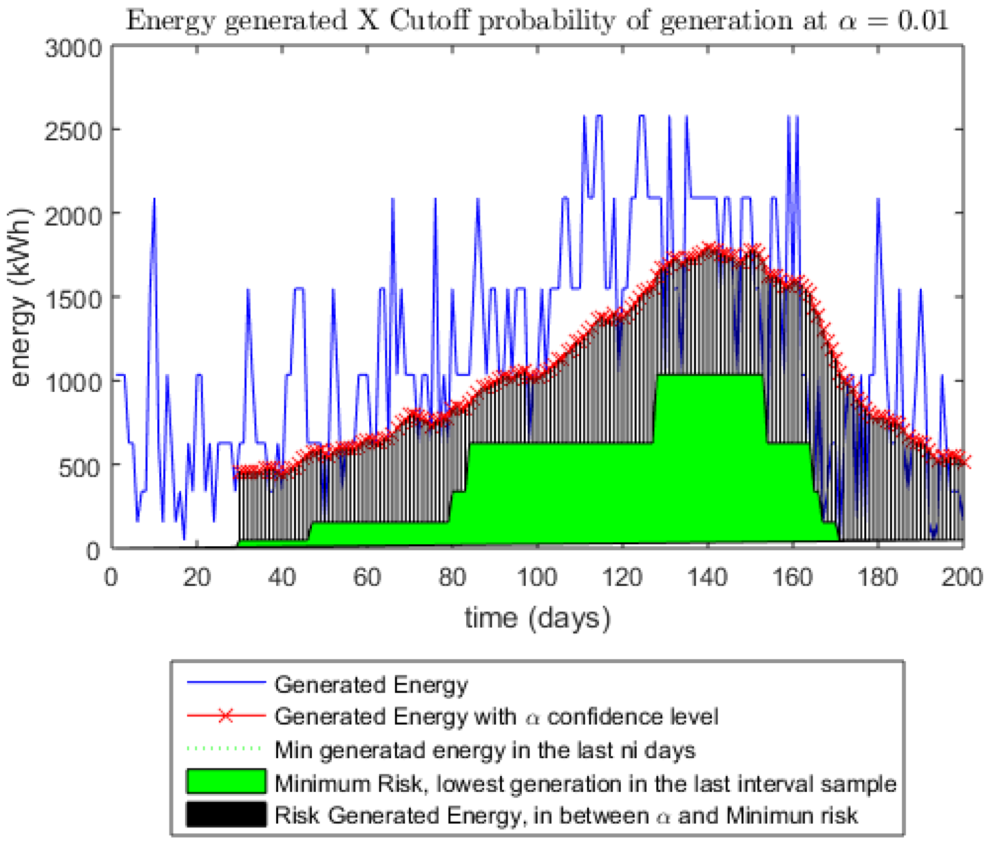
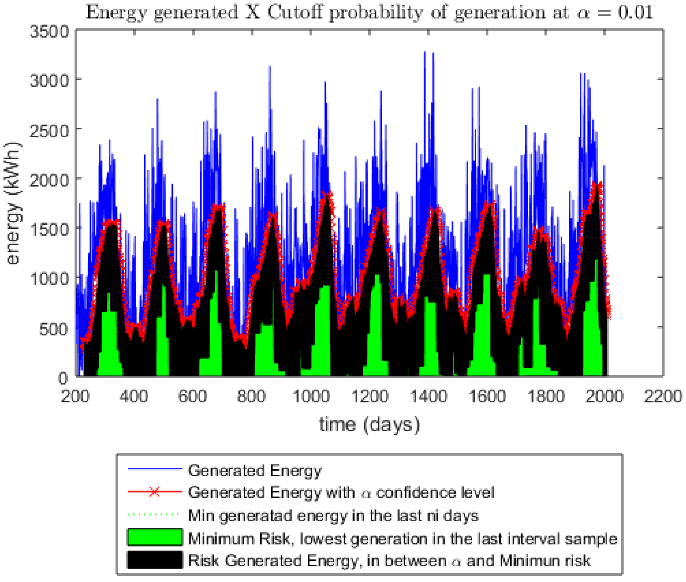
The Algorithm 3 yields two outputs: a set of equations that represent the wind behavior, and the forecast set of wind power generation. The forecast values are examined and used to find the most likely values, and the pessimist periods of generation along the year. Thus, a statistical analysis is performed onto forecasting. The analysis can be graphically represented, having in the x-axis the time, and in the y-axis, the power generated. Then the limits are drawn for the critical values, most unlikely values, and the risk generation periods in each part of the year.

Given a chosen significance level $\alpha$, and a moving window $w_n$ with $\Lambda$ samples, two particular situations are from interest here: the critical values (cutoff) from which the above values satisfy the chosen criteria of occurrence probability [55], and the lowest values in the last $\Lambda$ past points of a moving window $w_n$ where n is the number of windows. These two calculations indicate, in the forecasting values, the most likely happening values and the worst case region in the last windows. For example, let $\alpha =0.01$. Thus, it means it was chosen to have a 99% probability of having the forecasting values above the cutoff values in a one-sided z test given the past $\Lambda$ samples. Also, it means that it is expected to have 1% of the values under the cutoff. Under the cutoff region, the most cautious value is the lowest value in each past $\Lambda$ samples (or the minimum value in the past $w_n$ window), which represents a conservative forecast. The region between the cutoff slope and this cautious forecast slope is the risk taken for further decisions in the energy trade. Lower $\alpha$ values and longer window samples are most-likely to decrease the area between the cutoff and the conservative forecast. The length of these two variables keeps helpful information about the data seasonality to be used both from who sells than who buys the energy.

The procedure is resumed in Algorithm 4:

Algorithm 4: Determining confidence areas in the forecasting

Next section puts forward a case study for the proposed procedure from above.

3. Results

The implemented experiments aim at presenting the proposed method, that has as its main contribution to prove that it is possible to reduce the implementation time of wind-farms in Brazil, leading to a change in the Brazilian wind policy.

The experiments draw a comparison between the wind behavior in many different countries, investigating if they have a distinct wind behavior from Brazil that could justify its shorter implementation time.

Two kinds of experiments were proposed. The first focuses on the sample size necessary to forecast the wind energy generation, checking also the location influences. The second experiment focuses on how to use the forecasting to make confident decisions about the energy trade. The second experiment has as output a forecasting interval with a degree of confidence.

3.1. Experiment 1

Databases from NASA [32], NREL [33], and Petrolina were engaged in the experiments. The selections encompassed distinct countries, Brazilian regions and time sampling to assess the method suitability. Datasets of ten years durations were used with different training periods (from one to ten years) to forecast the remaining period of time. The procedure aims at comparing the wind speed measurements duration pointed out in Brazilian and international standards. To calculate the energy generation in each site we used the wind speed sample in m/s and the Equation (1). Algorithms 2 and 3 were applied in each site, performing the forecasts. Root mean square error (RMSE), and Mean Square Error (MSE) were used for validation, calculating the error in between the real wind power generation and the forecast using the proposed method.

Table 1. Forecasting error for different training samples and durations accounting for different data sources.

	NREL		Petrolina		NASA
Years	RMSE	MSE	RMSE	MSE	RMSE	MSE
1–10	4.82	23.22	209.83	41,146	147.67	21,808.53
2–10	5.57	31.09	197.21	43,420	145.95	21,302.85
3–10	6.16	38.06	211.95	40,219	142.74	20,375.66
4–10	6.16	38.00	212.26	45,712	143.05	20,463.44
5–10	6.02	36.25	213.46	45,259	140.53	19,750.16
6–10	5.82	33.92	213.48	45,844	136.10	18,523.47
7–10	6.02	36.27	215.22	46,174	134.44	18,076.17
8–10	5.82	33.87	215.37	46,320	131.74	17,357.86
9–10	5.61	31.50	188.93	46,385	130.84	17,119.88
10–10	5.48	30.03	203.80	34,409	130.41	17,006.85

presents the error using data sources (NASA, NREL, and Petrolina) for different training durations. Each sample has 10 years duration. The column Year represents the amount of data, in the sample, used for training and for forecasting. Thus, a value “2–10” in the column Year means it is used two years of a ten years sample to training the Algorithm 3. The same notation was used in all tables and figures.

It is noted that, in the same database, the error behavior is similar for different sampling intervals, but it changes depending on the location. Thereafter, the NASA data source was adopted, once it covers a larger number of locations worldwide.

Table 2. RMSE error on the testing set at different locations and durations.

Years Training/Testing	Brazil Natal	Brazil Janauba	Brazil Floripa	Scotland	Belgium Ghent	USA Florida	China Hongkong	Spain Barcelona	India Mumbai
1–10	156.98	109.18	264.57	113.48	304.89	163.76	188.79	254.80	33.57
2–10	148.37	111.04	295.65	120.57	298.44	155.04	201.18	238.70	32.75
3–10	146.37	110.69	240.41	114.87	256.56	150.63	227.75	251.25	32.12
4–10	147.85	117.51	265.34	116.84	262.73	154.05	214.93	223.29	32.72
5–10	148.13	116.72	266.84	116.02	243.29	158.75	256.12	251.75	33.37
6–10	146.49	118.29	267.19	114.45	252.05	160.25	251.60	252.13	33.44
7–10	147.80	120.17	252.10	111.98	240.86	162.41	231.67	247.94	33.31
8–10	147.66	117.82	250.46	113.54	233.07	163.05	231.11	250.20	35.65
9–10	146.75	115.88	247.24	114.17	229.59	161.51	233,16	250.71	35.74
10–10	146.75	117.60	269.15	113.93	229.59	159.98	182.48	249.91	35.90

cross-check different countries and three regions in Brazil, one in the extreme north, one extreme south and one in the middle. This aims at investigating if the wind behavior in Brazil is different from other countries. As could be noted, increasing the training sample and reducing the forecast horizon do not always decrease the forecasting error. Some cases showed better results with smaller training sample times. Between one and three years, it is not possible to say statistically that one training sample time is better than the other in the same site. Also, it was noted that the error in Brazilian wind sites is not an outlier when cross-checked with other countries error. The smallest set of errors was found in India and the greater one in Belgium. This is an evidence that the Brazilian wind policy is restrictive since the Brazilian wind behavior is similar to other countries ones.

Hence,

Table 3. RMSE Forecasting error for different training samples and durations in all Brazilian states.

	Years Training—Forecasting
Brazilian States	1–10	2–10	3–10	4–10	5–10	6–10	7–10	8–10	9–10	10–10
Sergipe—SE	127.96	123.37	125.89	125.84	123.62	121.33	122.74	120.68	119.86	119.86
Pará—PA	127.55	120.40	122.25	122.34	120.50	119.75	118.53	116.74	115.99	115.97
Minas Gerais—MG	75.90	73.29	71.59	76.13	77.15	73.16	72.79	71.70	71.90	71.83
Roraima—RR	9.74	9.24	8.65	8.69	8.98	8.99	8.78	8.46	8.40	8.39
Distrito Federal—DF	90.15	89.01	88.90	93.10	94.16	96.08	95.23	95.26	95.61	95.25
Mato Grosso do Sul—MS	128.90	115.50	107.95	112.17	107.95	106.13	101.87	94.58	93.15	92.49
Mato Grosso—MT	76.31	79.45	76.07	73.27	72.59	72.33	70.26	68.34	68.20	67.28
Paraná—PR	20.28	20.30	19.22	18.67	18.52	17.71	16.86	15.76	15.62	15.36
Santa Catarina—SC	174.84	179.78	182.72	175.85	173.85	177.60	177.17	173.55	171.82	170.38
Ceará—CE	153.68	144.66	146.27	145.04	149.11	148.80	153.48	150.15	151.25	151.00
Goiás—GO	116.58	111.69	110.89	107.78	109.40	107.04	105.92	105.94	107.45	107.27
Paraíba—PB	148.45	140.84	136.10	139.72	139.63	139.05	140.02	139.44	138.58	138.24
Amapá—AP	28.21	28.05	28.32	28.87	29.40	29.67	29.54	28.93	28.64	28.57
Alagoas—AL	138.19	129.79	130.71	128.36	130.22	131.47	131.32	131.37	133.12	133.12
Amazonas—AM	9.87	10.99	10.06	10.21	10.50	10.48	10.27	9.24	8.57	8.44
Rio Grande do Norte—RN	174.63	145.05	151.35	149.69	147.22	148.08	147.93	149.65	151.10	150.13
Tocantins—TO	82.00	76.25	81.40	81.88	84.53	83.67	86.12	87.01	87.74	87.25
Rio Grande do Sul—RS	98.67	85.15	89.10	87.67	82.29	74.89	74.44	74.15	69.93	69.24
Rondônia—RO	5.54	5.38	5.58	5.18	4.92	4.74	4.47	4.23	4.11	4.09
Pernambuco—PE	153.54	154.45	154.17	157.44	158.07	157.83	161.71	163.17	165.13	165.13
Acre—AC	11.48	7.78	7.34	7.03	6.64	6.51	6.09	5.99	5.41	5.24
Rio de Janeiro—RJ	70.64	73.96	70.69	72.05	72.26	74.83	70.96	70.47	69.02	68.99
Bahia—BA	87.98	84.56	89.36	90.15	91.51	91.25	88.26	88.96	89.33	89.33
Maranhão—MA	156.80	151.26	149.59	148.37	147.66	145.59	144.81	145.20	144.19	143.81
São Paulo—SP	63.76	60.60	59.81	58.76	57.39	55.61	56.75	53.73	53.81	53.26
Piauí—PI	102.21	100.09	99.65	99.38	100.20	99.55	99.18	97.82	96.94	96.82
Espírito Santo—ES	137.76	122.64	121.90	121.15	116.88	116.50	115.02	112.73	112.02	111.02

focuses on Brazilian sites. Ten years duration samples from all Brazilian regions were accounted for. As could be seen, changing the interval duration leads to the same magnitude errors. Some sites even presented smaller forecasting errors with one-year sample training set than with three-years.

Then, for each Brazilian state, it was cross-checked the 10 years forecasting with the real 10 years energy generation. One year of each sample was used to forecast the next nine years. Figure 2 shows the states box-plot. Each pair (forecast and real) represents a ten years sample, from 2007 till 2017 in each Brazilian state. The two letters abbreviations in the Figure 2 stands for the state name, (see Table 3). Each state has a pair of boxplots representing the real and forecast samples. As could be seen, these paired samples are quite similar. A hypotheses test between them showed in none of the states was possible to say that the real and forecast samples are different with a 95% confidence interval.

Thereafter, Figure 3 compares a real 10 years energy generation and its forecastings obtained from different durations of training. The training periods vary from 1 to 10 years of the sample. The number before the “y-10” represents the number of years used to train the algorithm to forecast the remaining data of the 10 years sample. It is easy to realize how similar are the real and forecasting samples, no matter how long it is the training period. This is an evidence of the method robustness to deal with wind energy forecasting.

The experiments performed did not show any evidence that Brazil could not adopt an international standard, and reduce the time for wind enterprises approval to one year rather than the current three years.

3.2. Experiment 2

Next experiments perform analysis about how the forecasting could be used to improve the confidence in energy trades, devising different levels of risk into the forecasting, assisting the stakeholders’ decision. Here, was used a wind speed dataset (m/s) from NASA’s database [32], in the Brazilian state Sergipe.

First, it was selected one year of this database, splitting 10% of the data for training and 90% for testing the forecast. Experiment 1 implemented Steps 1 to 3 from the proposed procedure in Figure 1. Now, Experiment 2 implements also the Step 4, that devises the confidence values into the forecasting, accounting for the last window of forecasting. This window move on time and, for each new value forecast, it is analyzed the set of data forecast in the last window.

Figure 4 considers the year 2007 in Sergipe’s dataset, and $\alpha =0.01$. In that figure, the wind behavior is represented by the energy generated, that is Step 3 output. The blue slope represents the real energy generated in the wind site, and the red slope is the forecast energy. In black, it is shown the slope of the cutoff values with 99% occurrence probability in the last 30 days window data. That means, considering the last 30 days, the next energy generation value have 99% of chance to be higher than the value in the black slope (the cutoff value). Just 1% of all samples are expected to be under that line. That window was adjusted to a monthly interval, but could be set to any lag time at decision maker convenience. This figure allows to analyze the forecasting against the most likely occurrence probability. The generation above the cutoff slope is the profitable risk, the values that the generation company is risking to gain. It is the optimistic risk scenario.

The black line (cutoff values) is the generated energy with $\alpha$ confidence level, considering the last forecast windows. Pinpointing this values reduces forecast volatility, once they represent the most likely value to happen, giving low importance to the noise and outliers in the prediction. The output is a more reliable value of forecasting. This cutoff values can be used by the energy trader to know the likely scenario of energy generation in the wind farm through the year.

Then, Figure 5 complements the Figure 4 with two new decision areas: the pessimist risk (green) and decision risk (black). The green line in the figure represents the lowest generation value in the last 30 days windows sample. Thus, the green area is the most pessimist generation in the last window sample, or the safest generation known in the last windows. The black area in between the green and red line is the decision risk area. The wind prospected sites with the smallest black area are the ones with the highest certainty in the energy generation. When the company already has the wind power plant implemented, this black area helps the decision maker to know when it is more risky to sell energy, and when is necessary to take into account other measures to mitigate the risk, for example, buy from another source of energy. In an auction situation, it helps to know what kind of procurement is more indicated to that site due the seasonality generation behavior. Also, it helps in formulating the bids limits once the bounds of the minimum energy generation are addressed. For example, an amount contract auction could not be indicated from the year ending to the beginning season once there is a higher possibility of zero generation at that period (no green area). Instead, the middle year has a bigger green area denoting a higher probability of generation where there is reduced chance of no generation.

Then, the whole procedure is extended to a 10 years sample, from which the first year of training was used to forecast the next 9 years of energy generation. This aims at planning in the long term. The same wind site from Sergipe was used. Figure 6 shows the result.

Figure 6 green areas represents the energy generation minimum risk, the red slope represents the most likely energy generation, and the blue one represents the 10-years real generation from 2007 to 2017. It is realized the wind seasonality through the year, with windy winters and little-wind summers. The green areas sum points out to the stakeholders the minimum energy generation expected for this wind site in the long term, and the sum of the area under the red slope represent the likely generation expected along these ten years. This information gives to the stakeholder the optimistic and pessimist scenarios of generation. Then, a minimum operator is used to summarize these ten years forecasting in just one year. Thus, the Algorithm 4 calculates, for each day of the year, the minimum value occurred in all forecasting years. The procedure is repeated for the minimum risk and to the cutoff values, giving a concise and cautious interpretation of the forecasting.

4. Discussion

EU approved in June 2018 the final agreement for decarbonizing its energy sector [56]. This is one of many efforts to reduce fossil fuel consumption worldwide. Indeed, migrating for a greener energy matrix have been the present days’ challenge, and it is better as fast as the countries move in that direction. However, different countries devise distinct policies to drive its energy market. This study aims at helping this energy matrix change in Brazil, that even with up to 60% of renewable sources, can become even greener and cheaper through fostering on wind energy. It was realized that other countries adopted a better policy that allows to implement the wind farms in a shorter time. Hence, it was investigated if it is possible to reduce the wind farms implementation time in Brazil and how. This topic is an open issue in literature, lacking on meaningful researches. This work focused on wind energy growth since it is cheaper, renewable and more abundant than other sources. Its main drawback is it stochasticity, that here it is overcome with a robust forecast method. This study has achieved three main contributions:

• Reducing the wind farm implementation time in Brazil:

Experiment 1 Section 3.1 investigated the wind behavior in Brazil, checking its similarity to other countries. It was implemented the steps 1 to 3 from the proposed method in Figure 1. From the results can be concluded that the Brazilian wind behavior is similar to the ones in countries adopting the standard IEC 61400. It was investigated also the sample size influence into the forecasting. Thus, it was examined the forecast quality and its relation with the training sample length in the 27 Brazilian states, and 6 other countries. It was used samples with 1 to 10-years duration to forecast the next years’ generation. The RMSE error was low in all the cases, and increasing the sample length from 1-year to 3-years did not reduce significantly the RMSE forecasting errors. Indeed, in 6 (SC, AP, AM, BA, MT, PR) of the 27 Brazilian states, the error had an increment using training samples of 2 and 3-years duration when compared at 1-year duration sample (Table 3). Now, consider the training periods of 1 and 3-years duration in all Brazilian states. The average percent difference between the respective RMSE forecasting errors was 5.36%, taking these two durations (Table 3). However, this 5.36% imprecision is insignificant comparing with the benefits of reducing with two years the wind farm implementation time. The Brazilian inflation target is 4.5% per year, the last 3 years inflation was 21.21% [19], and the last wind energy auctions offered a 400% reduction in the actual Brazilian energy price [3,4]. These indexes overcome this 5.36% difference in reducing the wind-farms implementation time in Brazil from 3 to 1 year. To the government, it is more effective to loosen the wind energy regulation, admitting 1-year duration samples to concede the building approvals. This will make the wind farms more attractive to the entrepreneur, fasten the Brazilian energy price reduction, and align Brazilian policy with the best international policies. If it is necessary, the government can devise a transitory reduction index of 5.36% to offset the expected amount of energy in the prospected site. Thereafter, the wind farm can claim this index review when the farm starts its energy generation. That keeps the balance, minimizing the wind farm implementation time without harm to the government conservative position. Both solutions, reduce the wind sample size to one year or include a transitory reduction index, could be easily implemented in the Brazilian wind policy with great benefits to the market. The whole market is benefited from this policy change, the government is benefited by bringing investments and new technology, the market by encouraging competition, and the final consumer by the energy price reduction.

2.

Introducing a reliable method to forecast the wind behavior:

This study also investigated the method capacity to represent the wind behavior. Real and forecast data behavior was cross-checked in Figure 2, identifying the samples’ level of similarity. That figure shows, with a high degree of confidence, that it is not possible to distinguish the real and forecast data, giving its high similarity. This indicates the method deals well with the wind stochasticity. RMSE error also denoted small values, reinforcing the statement. The statistical analysis in the FTS universe of discourse also contributed to the wind stochasticity representation and led to a robust forecast. The Step 3 approach was compared to other methods in [34], showing it outperforms in speed and precision the other FTS methods. However, this approach can suffer from the curse of dimensionality, increasing substantially the computational cost if a high-dimensional problem is designed.

The method is also suitable to represent linguistic variables such as $Temp=[$low, medium, high] and thus, can represent qualitative inputs. For example, a specialist advice, such as the Brazilian risk index of water shortage called Bandeira Tarifaria. Brazilian energy mix is highly dependent on hydroelectricity, so the government monitors the water shortage risk representing it in four levels: low, medium, high, and extra-high. Each level represents the government expectation of shortage, a truly fuzzy linguistic variable that should be interpreted by the energy market, reflecting on the prices. The market energy price increases and decreases depending on each level this index points out. The proposed method is perfectly suitable to represent this kind of situation and it could be explored in future works.

3.

Designing a risk index to treat the wind samples:

Proposed method in Step 4 introduces a risk representation into the forecasting. It allows representing a forecasting interval bounded by the most likely forecasting and the most cautious one. The most likely values are based on the cutoff values in the PDF slope for a given $\alpha$, and the most cautious slope represents the minimum value in a past window of data. Experiment 2 in Section 3.2 demonstrated this idea, extending the forecast duration from 1 to 10 years. Although the proposed method has shown a small RMSE error forecasting, the Step 4 improves the forecast representation, turning it from a point forecast to an interval forecast. This better represents the uncertainty, softening the wind volatility effects into the forecasting. The uncertainty representation is a key performance indicator to the energy market agents. The ratio between the likely forecast and the cautious one represents the spread of the possible values of forecasting. That ratio gives an uncertainty measurement, and it is helpful for designing the energy trader selling strategy. As near as it is this ratio to 1, more trustful is the expected energy generation, and as higher it is this number, as greater is the wind farm volatility. That helps to compare different wind sites, representing its risk and volatility in one index easily comparable.

5. Conclusions

This paper tackle some of the main issues of wind power industries. It was discovered it is possible to reduce with two years the wind farm implementation time in Brazil, bringing many benefits and no harm to the energy market. The experiments led to conclude that in the same wind site, a year, three years or even nine-year sample length are equally good and lead to a forecasting error of similar magnitude order. The benefits of a reduced time overcome the possible difference in the forecasting. The error seems to be more related to the wind behavior in the site than to the sample’s length. This can indicate that Brazilian wind policy imposes unnecessary constraints by establishing three years of sampling to approve the wind farms building licenses. Hence, it could be inferred that the Brazilian wind framework is less competitive than other markets adopting international standards. That disadvantage drives investments migration to other countries, indicating that adopting international standards could foster the Brazilian wind energy growth and make it more competitive worldwide.

The paper also showed that Clustering FTS methods are a good approach to represent wind behavior and its stochasticity. The proposed method shown to be flexible and trustworthy. Here, only the inputs wind speed and power generation were used in forecasting, but this method can use as many inputs as necessary, even linguistic ones and a mix of numeric and linguistic variables. Thus, further works could use many simultaneous generation sites to forecast distribution companies generation portfolio or use exogenous variables, like air humidity, solar radiation, and temperature to improve the forecasting. Another issue of interest to the market is the energy price. The approach designed here could be adapted to tackle that issue, having as output the energy prices.