Exact Solution of Heat Transport Equation for a Heterogeneous Geothermal Reservoir


Environmental Hydrogeology Group, Department of Earth Sciences, Utrecht University, Princetonlaan 8A, 3584 CB Utrecht, The Netherlands
Energies 2018, 11(11), 2935; https://doi.org/10.3390/en11112935
Submission received: 25 June 2018
/
Revised: 20 October 2018
/
Accepted: 24 October 2018
/
Published: 27 October 2018
(This article belongs to the Section L: Energy Sources)
Abstract
:An exact integral solution for transient temperature distribution, due to injection-production, in a heterogeneous porous confined geothermal reservoir, is presented in this paper. The heat transport processes taken into account are advection, longitudinal conduction and conduction to the confining rock layers due to the vertical temperature gradient. A quasi 2D heat transport equation in a semi-infinite porous media is solved using the Laplace transform. The internal heterogeneity of the geothermal reservoir is expressed by spatial variation of the flow velocity and the effective thermal conductivity of the medium. The model results predict the transient temperature distribution and thermal-front movement in a geothermal reservoir and the confining rocks. Another transient solution is also derived, assuming that longitudinal conduction in the geothermal aquifer is negligible. Steady-state solutions are presented, which determine the maximum penetration of the cold water thermal front into the geothermal aquifer.
1. Introduction
The generation and movement of the cold water thermal front inside a geothermal reservoir, due to reinjection of heat depleted water after power production, is a very important phenomenon to consider in designing the injection production well scheme of a geothermal power plant [1,2]. Reinjection of geothermal water after power generation is an essential procedure in maintaining the reservoir pressure, as well as the extraction efficiency, of a geothermal reservoir. But this in turn is responsible for cooling the reservoir with the passage of injection time. Geothermal reservoirs are frequently confined by impermeable rock layers above and below, which play a crucial role in the heat transport process that takes place due to the cold water injection. Besides advective and conductive heat transfer in the geothermal aquifer, another heat transfer process involved physically is heat loss to the confining rock layers. Being impermeable, the advective heat transport in the rock layers can be neglected, and the sole mode of heat transport consists of conductive flux to the rocks, due to the vertical temperature gradient between the geothermal aquifer and the rock media.
The phenomenon of the movement of a cold water thermal front in a geothermal reservoir has been studied analytically by a few researchers. A simple analytical model was developed by Bodvarsson [3] for the movement of the thermal front due to cold water injection, both for rocks with intergranular flow, as well as fracture flow. The author also discussed practical problems related to the siting of injection wells. Bodvarsson and Tsang [4] presented an analytical model to study the heat transfer phenomenon due to cold water injection into a geothermal reservoir with equally spaced horizontal fractures. A numerical study was also performed to verify the impact of the assumptions of the analytical model on the solution, which showed that the assumption of negligible horizontal conductive heat transport leads to an erroneous temperature distribution after a long time. Chen and Reddell [5] developed an analytical model for an aquifer thermal energy storage (ATES) system, which considered injection of hot water into a confined aquifer overlain and underlain by rock media. Two unsteady solutions were derived, one for a long time period and another for a short time period. The authors proposed a graphical technique for evaluating the aquifer thermal properties, like the longitudinal thermal conductivity and heat capacity of the aquifer, vertical thermal heat conductivity and the heat capacity of the caprock. Stopa and Wojnarowski [6] presented an analytical model, using the method of characteristics, to study the thermal front velocity of cold water injected into the geothermal reservoir. The authors considered the heat capacity and density of rock and water to be dependent on temperature, and neglected the longitudinal heat conduction. Yang and Yeh [7], Li et al. [8] and Yeh et al. [9] investigated the transient temperature behavior of an ATES system for a confined aquifer, bounded by rock media of different geological properties from above and below, by semi-analytical solutions using the Laplace transform. The authors used a numerical inversion technique, by numerical routine DINLAP, to derive their solutions, which approximates the Laplace inversion. An analytical solution for transient temperature distribution due to injection of heat depleted water into deep geothermal reservoirs is reported by Ganguly and Mohan Kumar [1], who developed a closed form analytical solution for the geothermal reservoir and also analyzed the sensitivity of a few parameters influencing heat transport in porous media.
Although there are a handful of analytical models existing in the literature, there are a very few which address the heterogeneity of a geothermal aquifer. Homogeneous aquifers are very rare in nature, and to present the actual scenario, it is essential to take into account the heterogeneity, because it has an important influence on the heat transport phenomenon in porous media. In a recent paper, Ganguly et al. [10] derived an analytical solution for a geothermal reservoir with block or layered heterogeneity. The present paper describes an analytical model of the transient thermal behavior due to injection of cold water into a geothermal aquifer with continuous heterogeneity, underlain and overlain by impermeable rock layers. Determination of the transient temperature distribution for a geothermal reservoir is necessary for designing the injection-production well scheme and fixing the flow rates through the wells. A one-dimensional heat transport equation in a porous geothermal aquifer, involving advective, conductive and heat loss (sink) terms, has been solved in order to derive complete and closed form solutions using the Laplace transform technique. As the solution is completely analytical, approximations or difficulties with the numerical Laplace inversion are avoided.
2. Mathematical Formulation
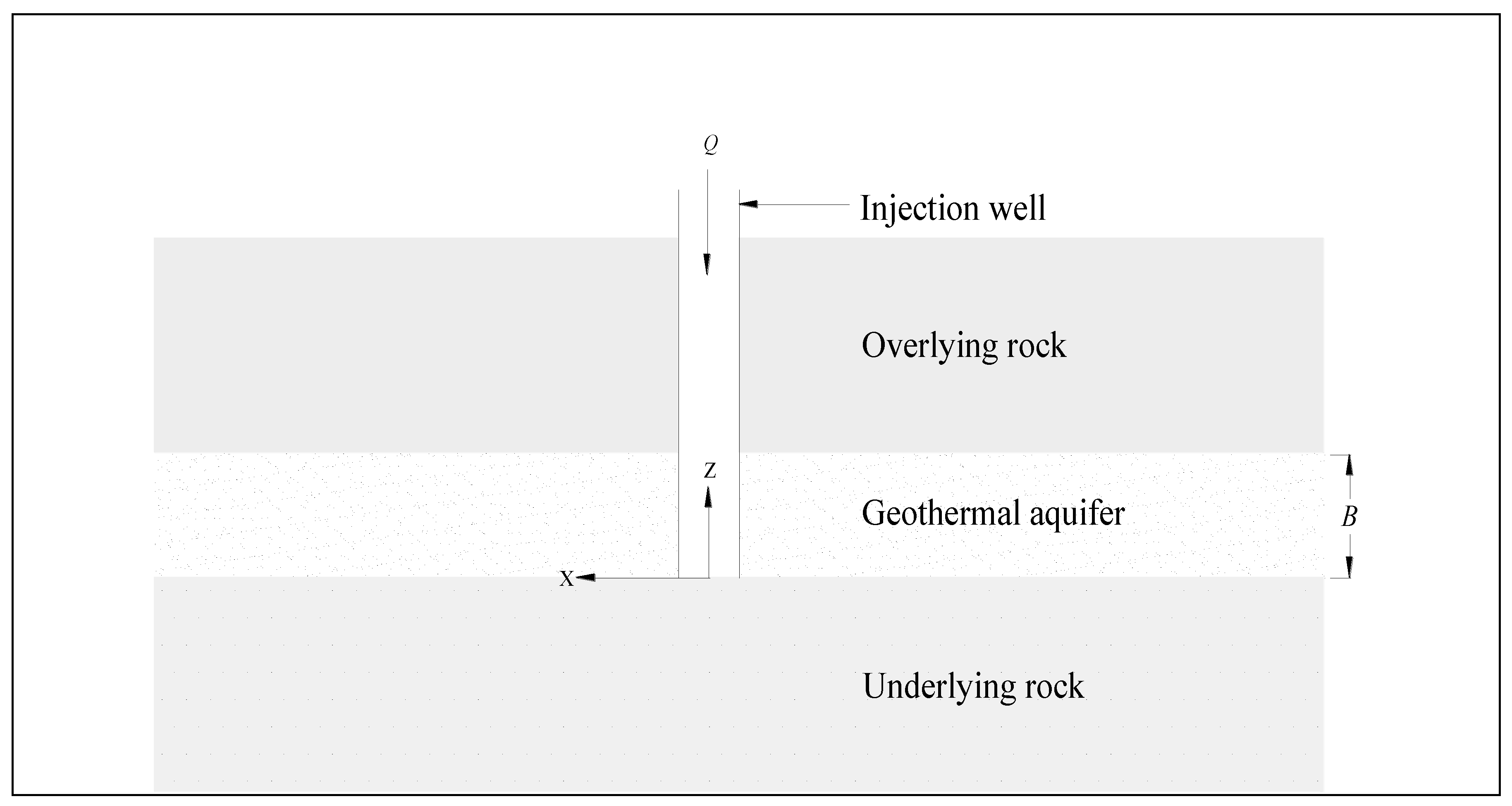
The mathematical model presented here is a set of coupled partial differential equations (PDEs), one for the confined porous geothermal reservoir and one each for the overlying and underlying rock layers. A schematic of the problem domain is shown in Figure 1. The coupling between the differential equations is ensured by the continuity of temperature at the interface of the geothermal reservoir with the confining layers. The one-dimensional heat transport equation for single phase fluid flow in a porous aquifer, involving advection, longitudinal conduction and heat transfer to the underlying and overlying rock media (source terms), is given by
where and are the densities of the rock and water, respectively; and are the heat capacities of rock and water, respectively; is the porosity of the geothermal reservoir; is the temperature, is the velocity of groundwater; q1 and q2 are the source terms of heat loss from the geothermal reservoir to the overlying and underlying rocks, respectively; is the injection time and represents the longitudinal direction. is the effective thermal conductivity porous media; is injection time and represents the longitudinal direction. The assumption of thermal equilibrium is applicable in the above differential equation.
The heterogeneity in the geothermal reservoir is expressed by a spatial variation of velocity [2,11,12] in a finite domain
where is the parameter of small magnitude accounting for the heterogeneity of the medium, is the flow velocity at the point of injection. The parameter is a dimensionless parameter of small magnitude. From Equation (2) it is evident that at the flow velocity through the porous media is at the injection well, which slowly and linearly increases along the distance due to the heterogeneity of the porous media. The small magnitude of the parameter and thus the parameter ensures that the velocity in the porous media is in the Darcy regime. The effective thermal conductivity () of the porous media, which is the dispersion parameter of the advection-dispersion in Equation (1), is considered to be proportional to [2], as suggested by [13,14]
The differential equation describing the heat transport in the overlying and underlying rock is
where subscripts 1 and 2 refer to overlying and underlying rocks, respectively. .
The source terms, i.e., the heat loss from the geothermal aquifer to the confining rock media at their interfaces , are modeled by Fourier’s law of heat conduction. If it’s considered that the heat flux to the rock media is proportional to the vertical temperature gradient between the geothermal aquifer and the rock layers, this leads to
where are the temperatures of the overlying and underlying rock. Substituting Equation (5) into Equation (1), we have the differential equation describing the transient heat transport phenomenon in the geothermal aquifer due to cold water injection
The initial and boundary conditions for the heat transfer Equation (6) for the geothermal aquifer in a semi-infinite domain are given by
The initial and boundary conditions for the heat transfer, Equation (4), for the overlying rock are
The initial and boundary conditions for the heat transfer, Equation (4), for the underlying rock are
The differential equations of heat transfer for the geothermal aquifer and the confining rock media are coupled through the boundary conditions in Equations (11) and (14), which denote the continuity of temperature at the interface of two media.
3. Analytical Solutions
3.1. The General Transient Solution
3.1.1. Solution for the Geothermal Aquifer
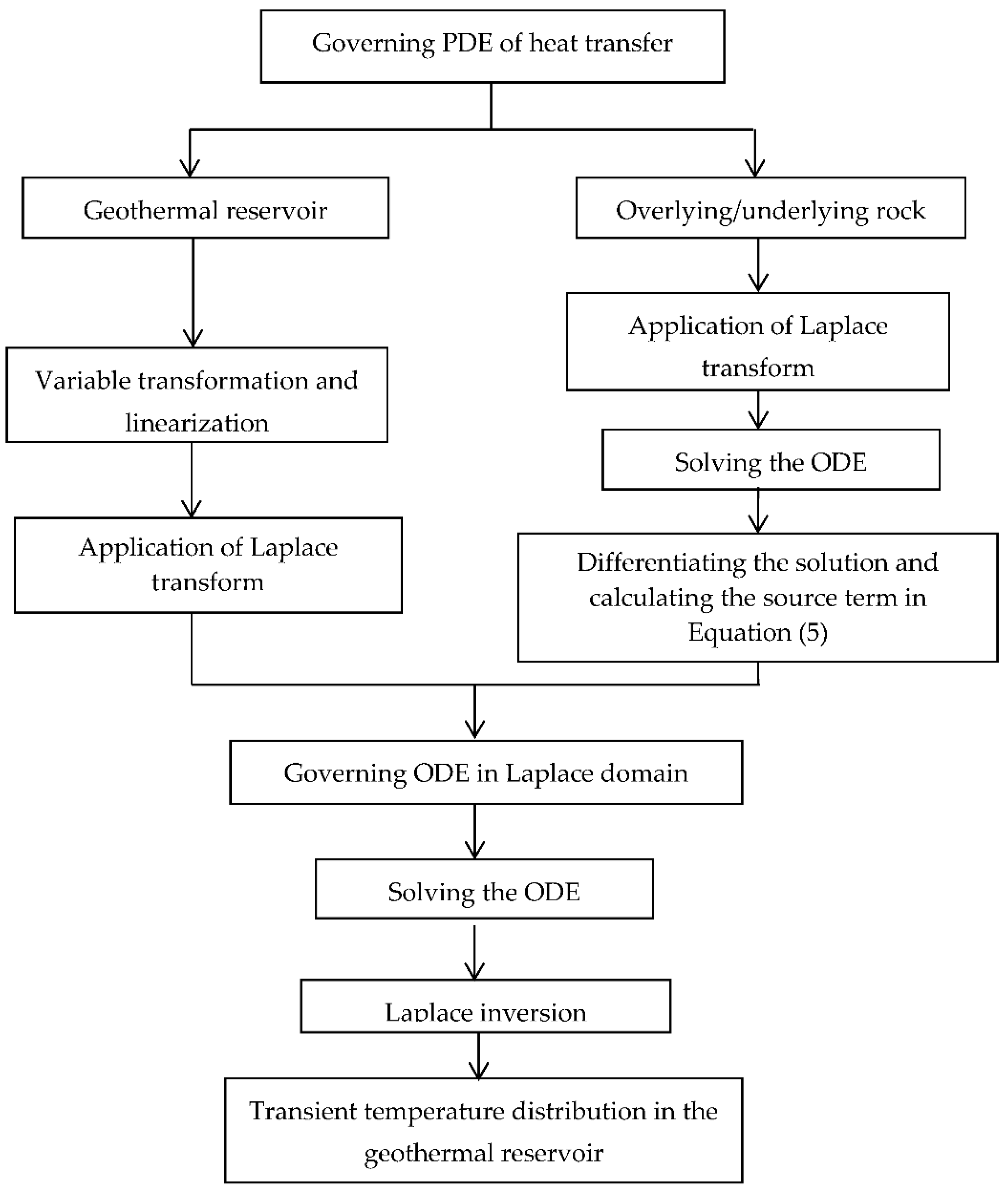
In order to solve the second order governing differential Equation (6) for transient heat transfer in the geothermal aquifer, a Laplace transform will be applied to the heat transfer equations for the overlying and underlying rocks given by Equation (4). The resulting ordinary differential equation (ODE) will be solved and the solution will be differentiated to obtain the temperature gradient at the interface of the geothermal aquifer and the rock media. The heat loss terms from the aquifer to the rock media are then determined using Equation (6), and substituted in Equation (3), which is then solved and inverted to obtain the temperature distribution in the geothermal aquifer. The whole solution procedure is presented as a flow chart in Figure 2.
Application of the Laplace transform to Equation (4) leads to
where is the Laplace transform of , which is defined as
where is a complex number.
Substituting the initial condition given by Equation (10) into Equation (16), the general solution of the ODE becomes
Since the solution is required to be bounded, the first term of Equation (18) should vanish to satisfy boundary condition (12). Constant is determined by using boundary condition (11), which gives
Hence the gradient of at the interface () of geothermal aquifer and the overlying rock is given by
Similarly, the gradient of at the interface () of the geothermal aquifer and the underlying rock is given by
A two-step variable transformation will now be performed with the aim to convert the variable coefficient PDE (6) to a constant coefficient one. The first variable transformation is for the distance in longitudinal direction, defined by
Application of the variable transformation to Equation (6) leads to
where and .
The initial and boundary conditions for Equation (23) in terms of the transformed space variable are given by
Using another variable transformation
Equation (23) can be written as
The initial and boundary conditions in terms of spatial variable become
Equation (28) is a constant coefficient second order PDE and hence the Laplace transform is applied to it. Substituting the source terms from Equations (20) and (21), the transformed ODE is given as
where
and
Equation (32) is derived using the initial condition in Equation (7). The general solution of Equation (32) is
where
Here . Boundary condition (9) requires . The unknown constant is determined by applying boundary condition (8), whose Laplace transform is
Hence the particular solution of Equation (32) finally can be written as
For practical values of all the parameters involved in and , (e.g., for values of parameters given in Table 1, the value of becomes 3.25 × 10⁻⁸). Hence Equation (38) can be reduced to
where is substituted in the above equation. Equation (39) can be expanded and written as
We now proceed to invert the solution in the Laplace domain. In order to facilitate the inversion, we make use of one integral result, given by [15]
Using the above integral result, Equation (40) can be written as
Application of the inverse Laplace transform on Equation (42) leads to the final result for the transient temperature distribution in a heterogeneous porous geothermal aquifer due to cold water injection, given by
Returning to the original space variable x, Equation (43) can be written as
where the lower limit of the integral has been changed to since the terms under integral sign requires
It is evident from Equation (44) that the second term exists due to the difference of the initial geothermal aquifer temperature () and temperature of the injected water (). Hence the larger the difference, the faster the cold water thermal front movement will be. The third and fourth terms in Equation (44) on the other hand, emerge due to the difference of the initial temperature of the geothermal aquifer and the confining rock media. If we assume the temperatures of the aquifer and the confining rock media are approximately equal (i.e., ), the above Equation (44) reduces to
3.1.2. Solution for the Overlying Rock
As the equations of heat transport for the geothermal aquifer and the overlying and underlying rocks are coupled, the next strategy will be to substitute Equation (43) into the general solution in Laplace domain for the heat transport equation in overlying rock, given by Equation (19), and invert the solution to obtain the two-dimensional transient temperature distribution for the overlying rock. By the substitution of Equation (42) into Equation (19) we have
Applying the inverse Laplace transform on Equation (46) and switching over to the original space variable , the above equation can be written as
As with the solution for the geothermal aquifer in Equation (44), it is also noticed that the second term in Equation (47) emerges due to the difference of the initial geothermal aquifer temperature and the temperature of the injected water. The third, fourth and fifth terms represent the contribution to the solution of the difference of the initial temperature for the geothermal aquifer and the confining rock media. Considering the initial temperature of the aquifer and the confining rocks to be almost equal (), the above equation reduces to
3.2. Transient Solution with Negligible Longitudinal Conduction
3.2.1. Solution for the Geothermal Aquifer
In certain geothermal reservoirs with very low thermal conductivity, the advective flux of heat transfer becomes much larger than the conductive flux. As a consequence the conductive heat transfer in those cases can be neglected. Mathematically neglecting the conduction term results in turning the second order PDE into a first order one, given by
Taking the Laplace transform of Equation (49) and substituting the source terms from Equations (20) and (21), we obtain
where Equation (7) has been used as the initial condition. Equation (50) is an ODE in the Laplace domain whose general solution is of the form
Using Equation (7) as the boundary condition we arrive at the particular solution of the ODE (50), given by
Since for all practical values of the parameters involved , Equation (52) can also be written as
Inverting the solution in the Laplace domain we arrive at the final solution for the transient temperature distribution in the geothermal aquifer in the case of negligible longitudinal conductive heat transport
The above Equation (54), in terms of the original space variable , can be written as
Like the previous case, we also see here that the second term of the solution is the contribution of the difference in the initial geothermal reservoir temperature and the temperature of injected water. The third and the fourth terms arise due to the difference of the initial geothermal aquifer temperature and that of confining rocks. In the case of an approximately equal initial temperature of the aquifer and the rock layers, the above Equation (55) simplifies to
3.2.2. Solution for the Overlying Rock
The same strategy is applied as before to derive the solution for the overlying rock media in the case of an aquifer with negligible longitudinal thermal conductivity. Substituting Equation (53) into Equation (19) we obtain
The solution in the Laplace domain is inverted to give the transient temperature distribution in the overlying rock in this case
Equation (58) in terms of the original space variable can be written as
The solution for the case of reduces to
4. Steady-State Solutions
The steady-state in the geothermal aquifer is reached when the heat transport flux by advection and conduction is balanced by heat loss to the over and underlying rock media. The steady-state solution is of great importance for predicting the maximum advancement of the cold water front, after which the temperature distribution in the aquifer remains constant. The region in the geothermal aquifer affected due to cold water injection can also be determined from it. The steady-state solution is developed here, making use of the final value theorem [16], which states
where is the steady-state value of a function and is the Laplace transform of .
Applying the theorem to the general transient solution (referred as GTS hereafter) for the geothermal aquifer in Equation (41), and writing the equation in the original variable , we obtain
Substituting the value of , the equation can also be written as
Substituting Equation (46) into Equation (19), and applying the final value theorem to that, yields again Equation (63), which is the steady-state solution for the temperature distribution in the overlying rock. The distance () penetrated by the thermal front, for any temperature at the steady-state, can be calculated for any value of the temperature ratio by rearranging Equation (63)
where . Similarly the steady-state temperature distribution in the geothermal aquifer for the negligible conduction case is found by applying the final value theorem to Equation (54), which again leads to the same Equation (64), which implies that the longitudinal conduction has no effect on the temperature distribution after a long time.
Like the previous case, substituting Equation (53) into Equation (19), and using the final value theorem, we obtain the steady-state solution for the overlying rock, which is also given by Equation (64). The steady-state solution implies that after a very long time, the geothermal aquifer and the rock layers attain the same temperature distribution throughout their domain in spite of the difference in their thermo-geological properties.
5. Results and Discussion
The analytical model derived in the previous section will be tested now by solving practical problems. The properties of the geothermal aquifer, the underlying and overlying rocks and the fluid properties required for testing the analytical model are listed in Table 1. The initial temperature of the geothermal aquifer (), the overlying rock () and underlying rock () are assumed to be 80 °C, 74 °C and 75 °C, respectively. Heat depleted water at a temperature of 20 °C () is injected at one end of the reservoir. The transient solutions derived in the previous sections for a geothermal aquifer (Equation (45)) and for the overlying aquifer (Equation (48)) are integral solutions. The integrals are evaluated using MATLAB by applying the Gauss−Kronrod quadrature technique for numerical integration. It is to be noted that although the upper limit of the integration extends to infinity, the numerically significant range is much smaller than that. To deal with this problem, the integral was tested for different upper limits, and the limit was fixed when no variation of the result was noticed with variation of the upper limit.
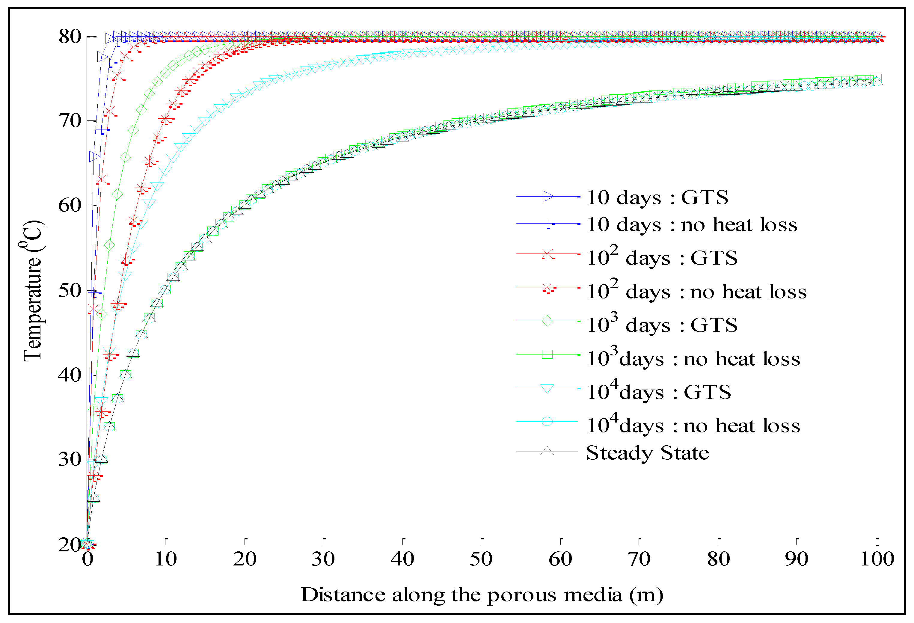
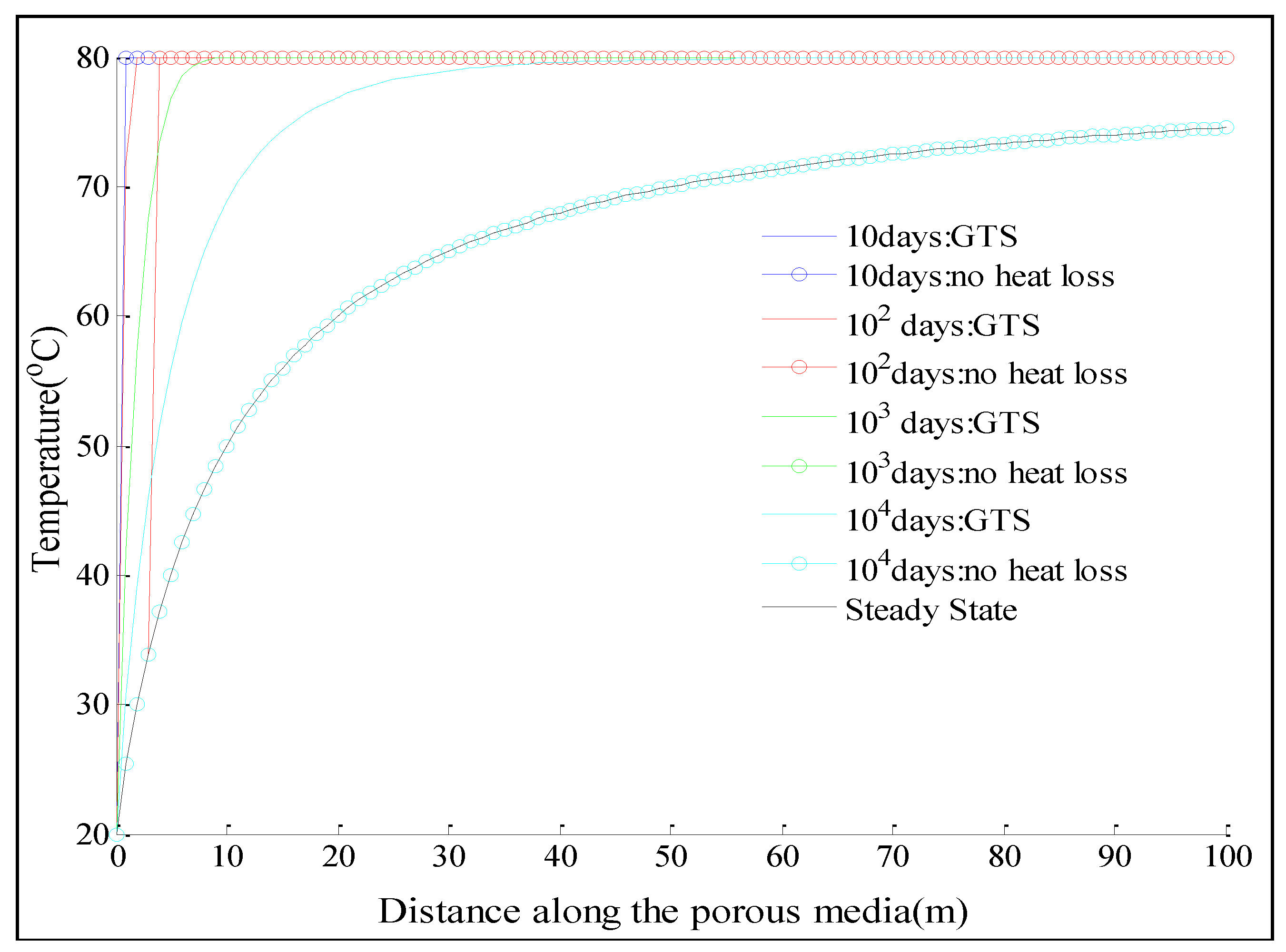
The temperature versus distance along the geothermal aquifer for the GTS at four different injection times is plotted in Figure 3, along with the temperature distributions for the no heat loss case given by Ganguly and Mohan Kumar [2]
The value of the heterogeneity parameter () is taken as 0.1 km−1 [12,13]. The curves show a nonlinear rising trend of the cold water thermal front, with the injection water temperature at one end and the initial geothermal aquifer temperature at the other. With the passage of injection time the thermal front advances through the geothermal aquifer and the aquifer temperature gradually declines until it attains the steady-state temperature distribution when the thermal front penetrates its maximum distance. After that, injection of cold water does not affect the temperature distribution further. The effect of a reduction in the geothermal aquifer temperature remains mostly concentrated near the injection well. Physically, the injected cold water extracts heat from surrounding rocks as it advances through the aquifer, and as the aquifer temperature gradually declines, the cold water gradually fails to extract enough heat to reach the initial geothermal aquifer temperature. When this effect reaches the production well, which is situated at a finite distance away from the injection well (the distance is less than penetrated at the steady-state), the temperature of the extracted water decreases, resulting in a reduction in efficiency of the geothermal reservoir. The steady-state solution given by Equation (63) is also plotted in Figure 3. Evidently the temperature distribution in the geothermal aquifer after a long time coincides with the steady-state temperature distribution, given by Equation (63).
The curves also show that the effect of heat loss on the transient temperature distribution is profound. Due to the loss of heat by conduction to the confining rock layers, the advancement of the cold water thermal front at a fixed injection time for the GTS is always less than the no heat loss case. The overall aquifer temperature is greater in the system with heat loss. The thermal front has advanced 5 m and 13 m in the GTS in 10 and 100 days, respectively, whereas it has advanced 7 m and 38 m for the no heat loss case. With the passage of injection time, this difference between the advancement of the thermal front increases, and the thermal front reaches the steady-state earlier in the case of no heat loss.
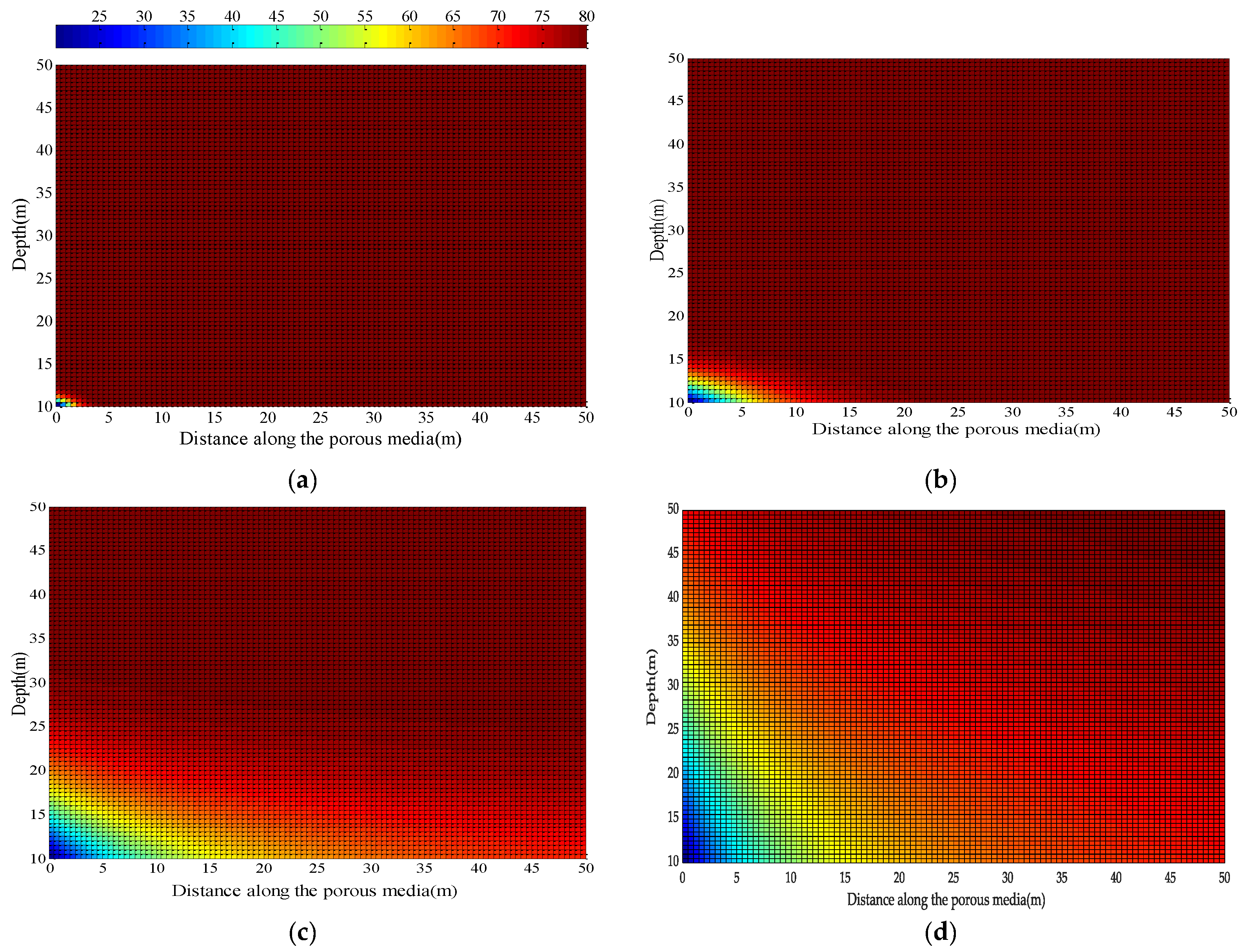
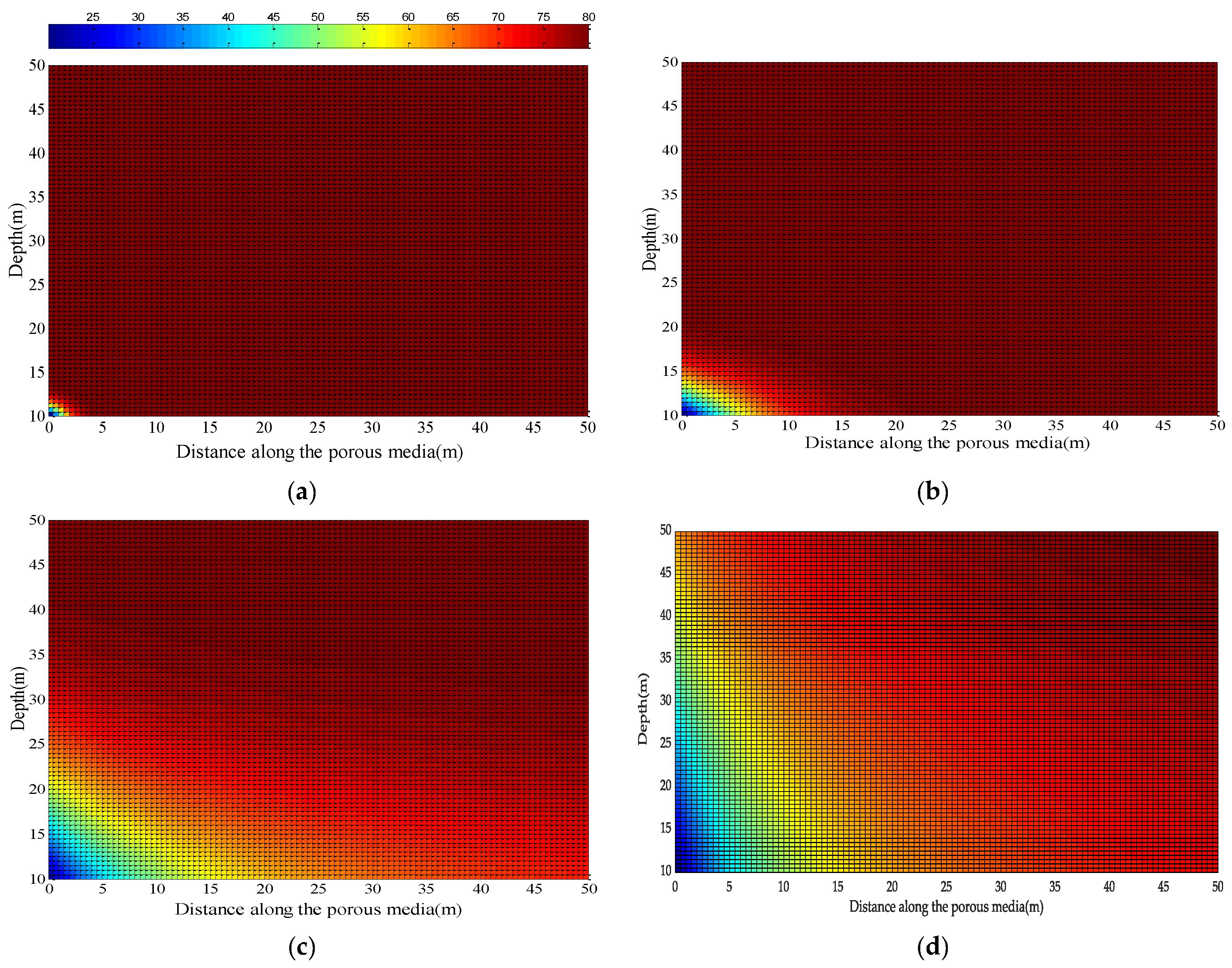
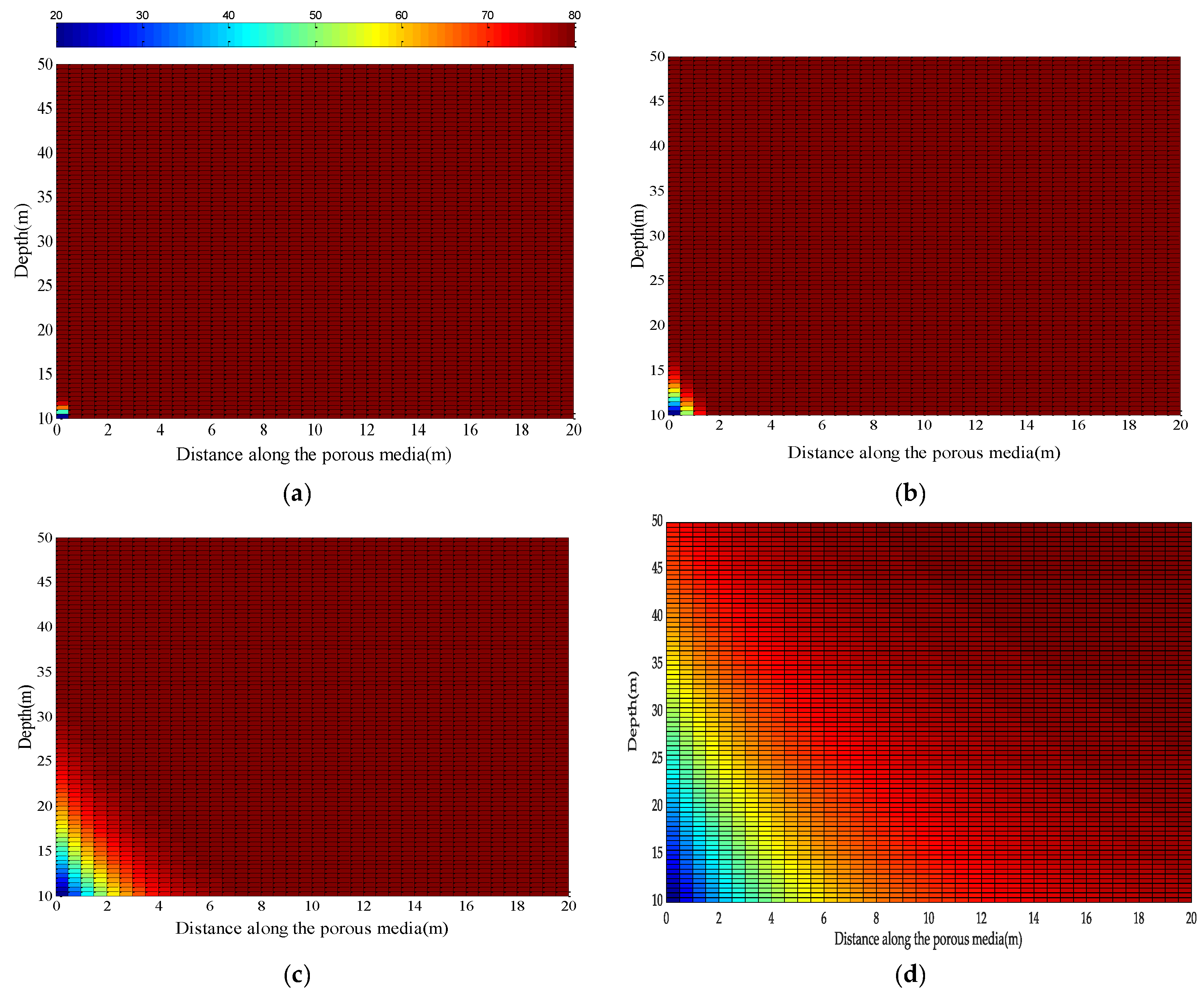
The two-dimensional transient temperature distributions in the overlying rock for the GTS, given by Equation (47), are shown in Figure 4a–d at four different injection times of 10, 100, 1000 and 10,000 days, respectively. The two-dimensional thermal front here also spreads with time, until it reaches steady-state. Figure 5a–d shows the temperature distributions in the overlying rock at the same injection times for a vertical thermal conductivity () of 2.5 W/m·K. Comparing the two figures, it becomes evident that due to higher vertical thermal conductivity in the second case, the cold water thermal front has advanced more and the overall temperature in the rock is also less than the first case. The advancement of the thermal front was 2 m, 5 m and 21 m at injection times of 10, 100 and 1000 days, respectively, in the first case, whereas the same for the second case was 3.5 m, 10 m and 30.5 m, respectively, at the same injection times. The results show that the vertical thermal conductivity of the overlying rock is an important parameter to consider in the computation of the transient temperature field in the rock media. The lager the value of the , the larger is the conductive heat flux in the overlying rock, which is responsible for faster movement of the thermal front and faster cooling of the rock media.
The transient temperature distributions in the geothermal aquifer for the case of negligible conduction are shown in Figure 6 at injection times of 10, 100, 1000 and 10,000 days. The solution for the case of no heat loss is given by [2]
for the same value of the heterogeneity parameter = 0.1 km−1, at the same injection times, and is also plotted in the same figure along with the steady-state temperature distribution in Equation (64). The temperature distribution after a long time coincides with the steady-state solution but the steady-state in this case is reached later than the GTS. As with the GTS, the thermal front for the no heat loss case is always ahead of the thermal front with heat loss, which is again due to the conductive transfer of heat to the confining rock media, which slows down the front movement. The overall aquifer temperature for the no heat loss case is also less than that with heat loss at a fixed injection time.
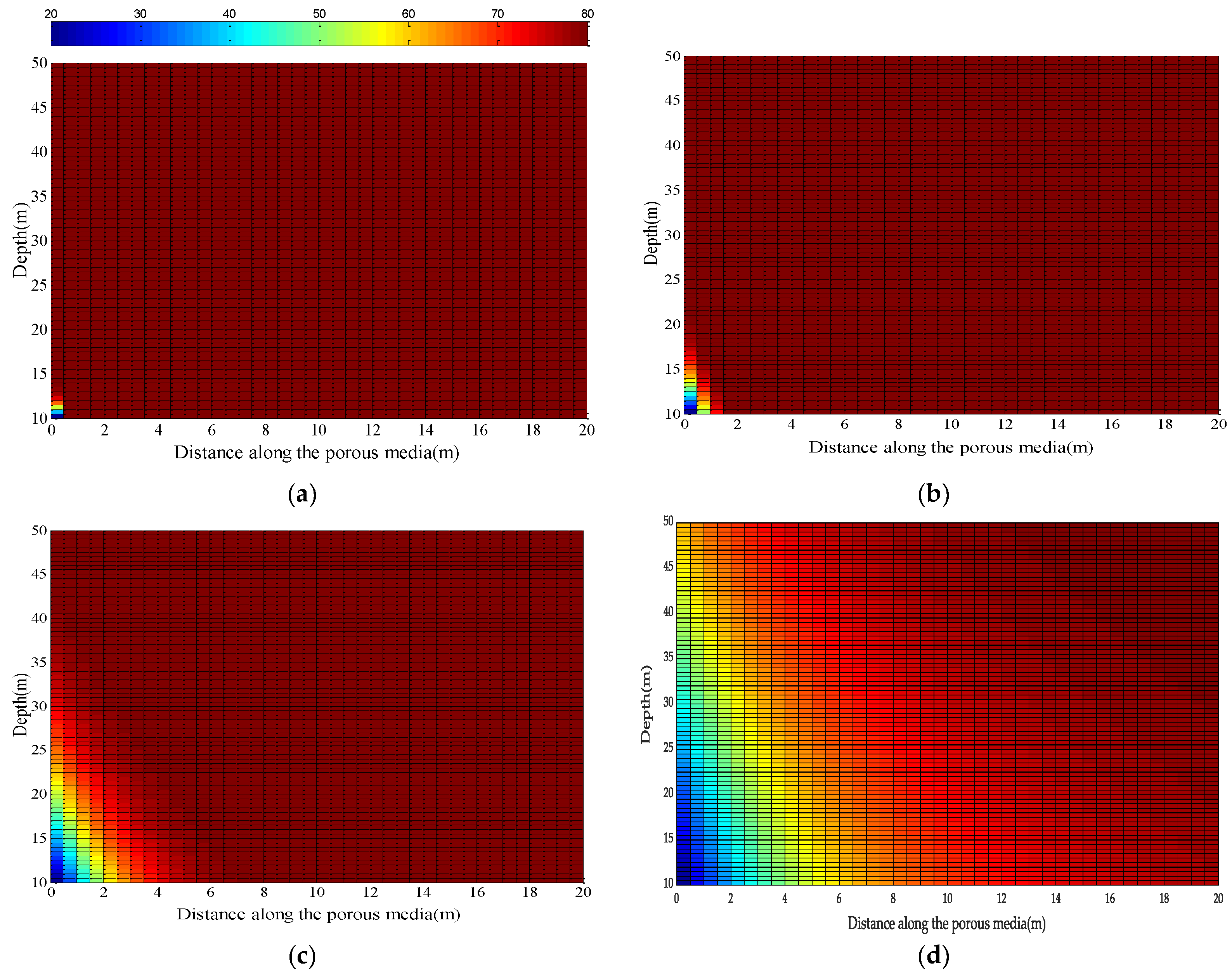
Figure 7a–d represents the temperature distributions in the overlying rock given by Equation (60) at injection times of 10, 100, 1000 and 10,000 days, respectively, for a vertical thermal conductivity of 1.2 W/m·K. The temperature distribution for the same, at the same injection times, for a vertical thermal conductivity of 2.5 W/m·K, is shown in Figure 8a–d, respectively. As with the GTS, it is also evident that due to the higher value of , the conductive heat flux to the overlying rock media increases, which results in faster advancement of the thermal front and cooling down of the rock media.
6. Conclusions
This paper reports an analytical model for the transient heat transfer phenomenon due to injection of cold water in a porous heterogeneous geothermal aquifer, overlain and underlain by impermeable rock media with different thermo-geological properties. The GTS included the heat transport modes of advection, longitudinal conduction and conduction to the over and underlying rock media due to a vertical temperature gradient. The Laplace transform was used as a solution technique. Transient solutions for the temperature distribution were developed for the geothermal aquifer as well as the overlying rock. A simpler solution was derived after considering the longitudinal heat transport to be negligible compared to the other modes. From the results it is evident that heat loss from the geothermal aquifer to the confining rock media plays a very crucial role in the transient heat transport phenomenon in a geothermal reservoir. The heat transport to the rock media helps to slow down the advancement of the cold water thermal front and cool the reservoir. The vertical thermal conductivity of the overlying and underlying rocks is an influential parameter in the transient temperature distribution of the rock media. The larger the value of the parameter, the larger is the heat flux to the rocks, which slows down the thermal front movement in the aquifer and cools it. The transient temperature distribution for an aquifer with negligible longitudinal conductivity is also derived, which also shows that the heat loss helps slow down the movement of the thermal front in this case. The advancement of the cold water thermal front for a system with heat loss is always less than that with no heat loss. Lastly, in spite of the assumptions made to represent the analytical model, it gives valuable insight into the temperature distribution and thermal front movement in a heterogeneous confined geothermal reservoir. The results presented here can serve as a reference solution for complex three-dimensional numerical models of a heterogeneous porous geothermal reservoir.
Funding
This research received no external funding.
Conflicts of Interest
The authors declare no conflicts of interest.
References
- Ganguly, S.; Mohan Kumar, M.S. Analytical solutions for transient temperature distribution in a geothermal reservoir due to cold water injection. Hydrogeol. J. 2014, 22, 351–369. [Google Scholar] [CrossRef]
- Ganguly, S.; Mohan Kumar, M.S. Analytical Solutions for Movement of Cold Water Thermal Front in a Heterogeneous Geothermal Reservoir. Appl. Math. Model. 2014, 38, 451–463. [Google Scholar] [CrossRef]
- Bodvarsson, G. Thermal problems in siting of reinjection wells. Geothermics 1972, 1, 63–66. [Google Scholar] [CrossRef]
- Bodvarsson, G.S.; Tsang, C.F. Injection and thermal breakthrough in fractured geothermal reservoirs. Water Resour. Res. 1982, 87, 1031–1048. [Google Scholar] [CrossRef]
- Chen, C.S.; Reddell, D.L. Temperature distribution around a well during thermal injection and a graphical technique for evaluating aquifer thermal properties. Water Resour. Res. 1983, 19, 351–363. [Google Scholar] [CrossRef]
- Stopa, J.; Wojnarowski, P. Analytical model of cold water front movement in a geothermal reservoir. Geothermics 2006, 35, 59–69. [Google Scholar] [CrossRef]
- Yang, Y.S.; Yeh, H.D. An analytical solution for modeling thermal energy transfer in a confined aquifer system. Hydrogeol. J. 2008, 16, 1507–1515. [Google Scholar] [CrossRef]
- Li, K.Y.; Yang, S.Y.; Yeh, H.D. An analytical solution for describing the transient temperature distribution in an aquifer thermal energy storage system. Hydrol. Process. 2010, 24, 3676–3688. [Google Scholar] [CrossRef]
- Yeh, H.D.; Yang, S.Y.; Li, K.Y. Heat extraction from aquifer geothermal systems. Int. J. Numer. Anal. Methods Geomech. 2012, 36, 85–99. [Google Scholar] [CrossRef]
- Ganguly, S.; Tan, L.; Date, A.; Mohan Kumar, M.S. Numerical investigation of temperature distribution in a confined heterogeneous geothermal reservoir due to injection-production. Energy Procedia 2017, 110, 143–148. [Google Scholar] [CrossRef]
- Kumar, A.; Jaiswal, D.K.; Kumar, N. Analytical solutions to one-dimensional advection-diffusion equation with variable coefficients in semi-infinite media. J. Hydrol. 2010, 380, 330–337. [Google Scholar] [CrossRef]
- Jaiswal, D.K.; Kumar, A.; Kumar, N.; Yadav, R.R. Analytical solutions for temporally and spatially dependent solute dispersion of pulse type input concentration in one-dimensional semi-media. J. Hydro-Environ. Res. 2009, 2, 254–273. [Google Scholar] [CrossRef]
- Scheidgger, A.E. The Physics of Flow through Porous Media; University of Toronto Press: Toronto, ON, Canada, 1958. [Google Scholar]
- Taylor, G. Dispersion of soluble matter in solvent flowing slowly through a tube. Proc. R. Soc. Lond. Ser. A 1953, 219, 186–203. [Google Scholar] [CrossRef]
- Gradshteyn, I.S.; Ryzhik, I.M. Table of Integral, Series, and Products, 7th ed.; Academic Press: Troy, NY, USA, 2007. [Google Scholar]
- Churchill, R.V. Operational Mathematics, 3rd ed.; McGraw-Hill: New York, NY, USA, 1972. [Google Scholar]
Figure 1.
Schematic representation of the confined geothermal aquifer with the injection well.

Figure 2.
Flow chart showing the analytical solution procedure of the governing partial differential equations (PDEs). ODE is ordinary differential equation.
Figure 2.
Flow chart showing the analytical solution procedure of the governing partial differential equations (PDEs). ODE is ordinary differential equation.

Figure 3.
Temperature distribution plots in the geothermal aquifer at different injection times for the general transient solution and the no heat loss case.
Figure 3.
Temperature distribution plots in the geothermal aquifer at different injection times for the general transient solution and the no heat loss case.

Figure 4.
Temperature distribution in the overlying rock for = 1.2 W/m·K at (a) 10 days, (b) 100 days, (c) 1000 days and (d) 10,000 days.
Figure 4.
Temperature distribution in the overlying rock for = 1.2 W/m·K at (a) 10 days, (b) 100 days, (c) 1000 days and (d) 10,000 days.

Figure 5.
Temperature distribution in the overlying rock for = 2.5 W/m·K at (a) 10 days, (b) 100 days, (c) 1000 days and (d) 10,000 days.
Figure 5.
Temperature distribution in the overlying rock for = 2.5 W/m·K at (a) 10 days, (b) 100 days, (c) 1000 days and (d) 10,000 days.

Figure 6.
Temperature distribution plots in the geothermal aquifer at different injection times for the negligible conduction case with and without heat loss.
Figure 6.
Temperature distribution plots in the geothermal aquifer at different injection times for the negligible conduction case with and without heat loss.

Figure 7.
Temperature distribution in the overlying rock for the negligible conduction case for = 1.2 W/m·K at (a) 10 days, (b) 100 days, (c) 1000 days and (d) 10,000 days.
Figure 7.
Temperature distribution in the overlying rock for the negligible conduction case for = 1.2 W/m·K at (a) 10 days, (b) 100 days, (c) 1000 days and (d) 10,000 days.

Figure 8.
Temperature distribution in the overlying rock for the negligible conduction case for = 2.5 W/m·K at (a) 10 days, (b) 100 days, (c) 1000 days and (d) 10,000 days.
Figure 8.
Temperature distribution in the overlying rock for the negligible conduction case for = 2.5 W/m·K at (a) 10 days, (b) 100 days, (c) 1000 days and (d) 10,000 days.


Table 1.
Parameters of the rock and fluid used.
| Parameter Name | Magnitude |
|---|---|
| Specific heat of the aquifer (Cr) (J/kg °C) | 2713 |
| Specific heat of the overlying rock (Cr1) (J/kg °C) | 1046 |
| Specific heat of the underlying rock (Cr2) (J/kg °C) | 800 |
| Density of the aquifer (ρr) (kg/m3) | 1047 |
| Density of the overlying rock (ρr1) (kg/m3) | 2650 |
| Density of the underlying rock (ρr2) (kg/m3) | 2600 |
| Thermal conductivity of the aquifer (λ) (W/m °C) | 2.4 |
| Thermal conductivity of the overlying rock (λ1) (W/m °C) | 1.5 |
| Thermal conductivity of the underlying rock(λ1) (W/m °C) | 2.59 |
| Porosity of the aquifer (ϕ) | 0.3 |
| Porosity of the overlying rock (ϕ1) | 0.10 |
| Porosity of the underlying rock (ϕ2) | 0.15 |
| Density of the geothermal fluid (ρw) (kg/m3) | 985 |
| Specific heat of the geothermal fluid (Cw) (J/kg °C) | 4180 |
| Initial temperature of the overlying rock T01 (K) | 343 |
| Initial temperature of the underlying rock T02 (K) | 338 |
| Vertical area of the geothermal aquifer (A) (m2) | 107 |
| Thickness of the aquifer B (m) | 5 |
| Thickness of the overlying rock b1 (m) | 60 |
| Thickness of the underlying rock b2 (m) | 50 |
© 2018 by the author. Licensee MDPI, Basel, Switzerland. This article is an open access article distributed under the terms and conditions of the Creative Commons Attribution (CC BY) license (http://creativecommons.org/licenses/by/4.0/).
Share and Cite
MDPI and ACS Style
Ganguly, S. Exact Solution of Heat Transport Equation for a Heterogeneous Geothermal Reservoir. Energies 2018, 11, 2935. https://doi.org/10.3390/en11112935
AMA Style
Ganguly S. Exact Solution of Heat Transport Equation for a Heterogeneous Geothermal Reservoir. Energies. 2018; 11(11):2935. https://doi.org/10.3390/en11112935
Chicago/Turabian StyleGanguly, Sayantan. 2018. "Exact Solution of Heat Transport Equation for a Heterogeneous Geothermal Reservoir" Energies 11, no. 11: 2935. https://doi.org/10.3390/en11112935
Note that from the first issue of 2016, this journal uses article numbers instead of page numbers. See further details here.