Hierarchical Control of Nonlinear Active Four-Wheel-Steering Vehicles

Abstract

A new type of hierarchical control is proposed for a four-wheel-steering (4WS) vehicle, in which both the sideslip angle and yaw rate feedback are used, and the saturation of the control variables (i.e., the front and rear steering angles) is considered. The nonlinear three degrees of freedom (3DOF) 4WS vehicle model is employed to describe the uncertainties originating from the operating situations. Further, a normal front-wheel-steering (2WS) vehicle with a drop filter of the sideslip angle is selected as the reference model. The inputs for the rear and front steering angles of the linear 2DOF 4WS, required to achieve the performances described by the reference model, are obtained and controlled by the upper controller. Further, the lower controller is designed to eliminate the state error between the linear 2DOF and nonlinear 3DOF 4WS vehicle models. The simulation results of several vehicle models with/without the controller are presented, and the robustness of the hierarchical control system is analyzed. The simulation results indicate that using the proposed hierarchical controller yields the same performance between the nonlinear 4WS vehicle and the reference model, in addition to exhibiting good robustness.

1. Introduction

The active four-wheel-steering (4WS) system is studied widely to improve the handling stability at high speeds, and the maneuverability at low speeds. With the emergence of intelligent vehicle systems (IVS), the 4WS system can also be used to solve the path tracking problem to ensure that the vehicle can follow the scheduled route, and its algorithm is mainly about determining the required steering angle to adjust the dynamic turning point on the road curvature center [1,2,3]. Hitherto, some control strategies and methods have been proposed to improve the aforementioned control goals, such as fuzzy, adaptive, feedforward, feedback, optimal, H_∞, sliding mode, decoupling, and neural network controls, as well as μ synthesis.

A yaw stability controller based on fuzzy logic was proposed, which took the yaw angular velocity error, steering angle given by driver, and side slip angle as input, calculated the additional steering angle as output, and compared with the existing fuzzy control system with two inputs of the yaw angle and yaw angular velocity. The results showed that the proposed fuzzy yaw controller had better performance [4]. Considering the rear wheel steering resistance moment, the H₂/H_∞ mixed robust controller was designed to track the desired yaw rate, and can be obtained according to the variable transmission ratio strategy [5]. Applying the yaw rate tracking strategy to the 4WS vehicle and considering the resistance moment of rear wheel steering, the H₂/H_∞ infinity hybrid robust controller was designed and the stability control of 4WS vehicle was studied [6]. A μ synthesis robust controller was designed to overcome the model uncertainty [7]. Considering the velocity changing, a linear parameter varying (LPV) controller was designed to improve the handling stability, safety, and comfort of the 4WS vehicle [8]. A high-level control redistribution method based on LPV control framework was adopted to realize torque vectorization and steering, which can ensure the speed and path tracking of the four-wheel independently-actuated (4WIA) vehicle in the case of one or even several wheeled motor failures or performance degradation [9]. Using the preview theory, robust theory, and adaptive path following, the 4WS vehicle can exhibit a good path tracking capability in both the longitudinal and lateral directions [10]. Based on the singular boundary theory and Lyapunov stability theory, the uncertainty of the 4WS vehicle was debated [11]. Combined with the linear programming algorithm and the improved sliding mode algorithm, a joint control strategy combining the exponential reaching law with the saturation function was proposed. The strategy can control the side slip angle, yaw speed, and yaw moment of the vehicle well to improve the handling and stability performance of the vehicle significantly [12]. Based on sliding mode control, an integrated control system with 4WS and direct yaw moment control (DYC) was proposed to improve vehicle handling stability [13]. A fast terminal sliding mode controller was designed to suppress the external disturbance of the steer-by-wire (SBW) system. Considering the unstructured and structural uncertainties, a robust controller was designed by using the synthesis method; the controller order reduction was realized based on Hankel-Norm approximation, and the extended Kalman filter was used to estimate the sideslip angle [14].

In addition, relative investigations have shown that the decoupling control of the vehicle steering characteristics can improve the vehicle’s safety, driving, and even exhibit accurate trajectory tracking because of the vehicle’s individual control of the lateral and yaw motions [15]. A robust triangular decoupling control strategy was proposed to decouple the front axle acceleration from the yaw rate [16]. A lateral-force observer based on the disturbance observer theory was developed, aiming to overcome the fragile robustness of the decoupling control for road conditions, and used along with the yaw-moment observer in a small-scale electric vehicle. Further, the robustness against parameter variation was improved [17]. The necessary and sufficient conditions for the solution of diagonal decoupling were presented, and the vehicle model (lateral plus roll dynamics) was implemented to control the steering angle and sideslip angle of the vehicle independently, using a static state feedback law with a static pre-compensator [18]. An asymptotic decoupling control for the 4WS vehicle based on an easy measurement feedback was introduced. Its control inputs were the front wheel steering angle, and the torques of front and rear wheels; further, the H∞ optimization method was used to derive the desired eigenvalues [19]. Pre-compensation decoupling with H_∞ performance control for a 3DOF nonlinear 4WS vehicles was studied to consider the influence of disturbances on the output under the H_∞ index. The results showed that the longitudinal velocity, lateral velocity, and yaw rate can be controlled independently, and the drivers can steer rapidly [20]. A simple decoupling subsystem consisting of longitudinal, lateral, and yaw dynamics is derived by choosing the combination of longitudinal acceleration/braking force and steering angle of front and rear wheels as the virtual control input [21].

However, compared with diagonal decoupling, triangular decoupling is more complicated, particularly for uncertain systems [22]. Further, it is difficult to build fuzzy rules in all situations for fuzzy control algorithms, and the adaptive control is suitable for the slow time-varying system that is vastly different from the actual steering system whose parameters may change quickly [23]. In addition, the control strategies for a 4WS system can be divided into two types: one is to make the sideslip angle zero, corresponding to trajectory preserving problem, the other one is to track the desired yaw rate. Most studies on the control of 4WS vehicles usually aim to determine the rear wheel steering angle based on the certain front wheel steering angle, and compare the response of 4WS vehicle under the inputs of the front and rear wheel steering angles with that of the 2WS vehicle.

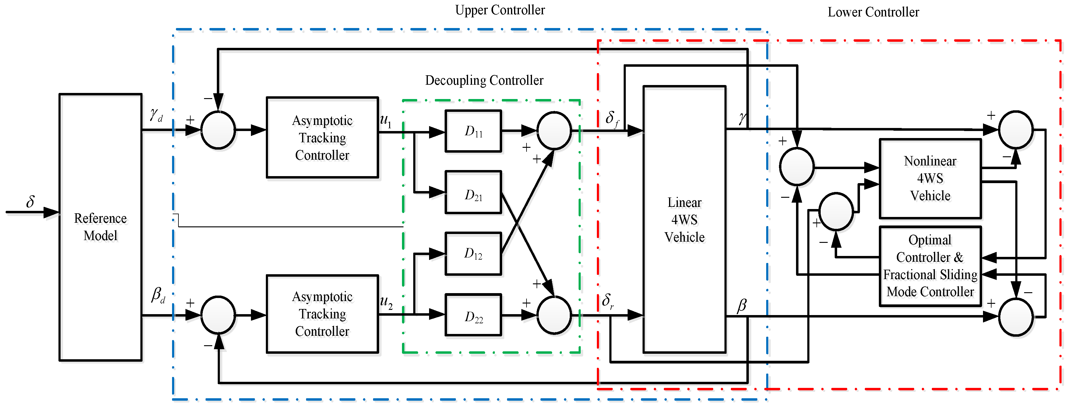
The novelties of this study are as follows: (1) The reference model is obtained by filtering the sideslip angle of a normal 2WS vehicle, which is very different from past practices. (2) According to the 2WS reference model, the front and rear wheel steering angles of linear 4WS vehicle are determined simultaneously by the decoupling controller, and its response is consistent with that of the 2WS reference model completely. (3) Considering that it is very difficult to design controllers directly by using nonlinear models, a new hierarchical controller is proposed in this paper. Firstly, the upper controller controls the linear 4WS model to have the same response as the 2WS reference model. Then the lower controller controls the nonlinear 4WS model to have exactly the same response as the linear 4WS. (4) The upper control strategy, including the decoupling controller and asymptotic tracking controller, is designed to provide the standard input for the linear 4WS vehicle model. The former is to decouple the sideslip angle and yaw rate from each other, which can obtain the required front and rear wheel steering angles. The latter is to control the linear 4WS vehicle model to track the reference model completely. (5) The lower control strategy, including the optimal controller and fractional sliding mode controller, is designed to remove the adverse effects of the state errors between the linear 2DOF and nonlinear 3DOF 4WS vehicle models. The former is to eliminate the state error caused by the different initial states. The latter is to eliminate the state error caused by the uncertainty.

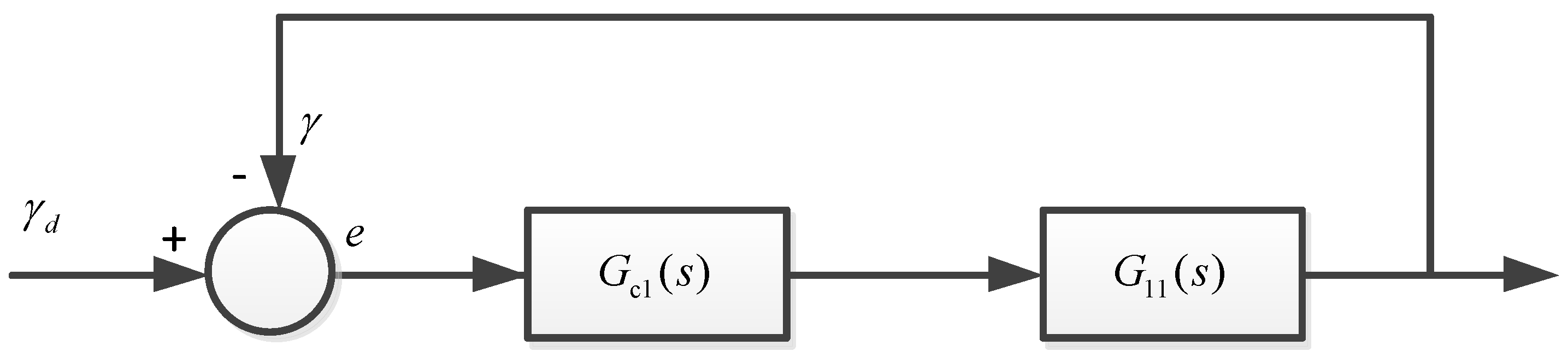
The subsequent parts of this paper are organized as follows: In Section 2, the vehicle models, including the nonlinear 3DOF 4WS/2WS model, the linear 2DOF 4WS/2WS model, and the reference model are presented. The hierarchical control strategies, including the upper control strategy (i.e., the decoupling and the asymptotic tracking control) and the lower control strategy (i.e., the optimal control and the fractional sliding mode control), are described in Section 3. The comparison of the simulation results of the linear 2DOF 2WS vehicle, reference model, nonlinear 3DOF 2WS vehicle, real vehicle with the hierarchical controller and linear 4WS with linear quadratic regulator (LQR) controller are reported in Section 4. Finally, the conclusion is summarized in Section 5.

2. Model Description

We consider three types of vehicle models for the hierarchical control system. The first one is a nonlinear 3DOF 4WS/2WS vehicle model used to describe the system uncertainty, which is controlled by a lower controller to ensure the system robustness. The second one is a linear 2DOF 4WS/2WS vehicle model controlled by an upper controller, which can supply the standard inputs to 4WS vehicles. The last one is a reference model to provide the desired yaw rate and sideslip angle.

2.1. Nonlinear 3DOF 4WS/2WS Vehicle Model

The 4WS vehicle model considering the lateral, yaw, and roll motions is given by

$$\{\begin{array}{l}{I}_z\dot{\gamma }-I_{xz}\ddot{\varphi }=2a{F}_f-2b{F}_r\\ m{u}_x\left(\dot{\beta }+\gamma \right)+m_s{h}_s\ddot{\varphi }=2F_f+2F_r\\ I_x\ddot{\varphi }-I_{xz}\dot{\gamma }+m_s{h}_s{u}_x\left(\dot{\beta }+\gamma \right)=\left(m_{s}g{h}_s-k_{\varphi }\right)\varphi -c_{\varphi }\dot{\varphi }\end{array},$$

(1)

where I_z is the moment of inertia of the vehicle about the z-axis, I_x is the roll moment of inertia of the vehicle body about the x-axis, I_xz is the moment of the inertia product, γ is the yaw rate, ϕ is the roll angle of the vehicle body, a and b are the distances from the centroid to the front and rear axle, F_f and F_r are the lateral forces of the front and rear wheel respectively, m is the vehicle mass, u_x is the longitudinal speed of the vehicle, β is the sideslip angle, m_s is the mass of the vehicle body, h_s is the distance of the body centroid to the roll center axis, g is the gravitational acceleration, k_ϕ is the sum of the roll stiffness of the front and rear suspensions, and c_ϕ is the sum of the roll damping of the front and rear suspensions.

Considering the nonlinearity of the tires, the lateral forces of the front and rear wheels can be expressed as follows [17]:

$$F_i=\phi D_i\sin (C_i\arctan (B_i(1-E_i)\frac{{\alpha }_i}{\phi }+E_i\arctan (B_i\frac{{\alpha }_i}{\phi })))\hspace{1em}i=f,r,$$

(2)

where

$${\alpha }_f=\beta +a\gamma /u_x-R_f\varphi -{\delta }_f,{\alpha }_r=\beta -b\gamma /u_x-R_r\varphi -{\delta }_r,$$

(3)

φ is the road adhesion coefficient (ranging from 0.2 to 1), B_i, C_i, D_i, E_i are the coefficients, α_i is the slip angle of the wheel. R_f and R_r are the roll deflection coefficients of the front and rear axles, respectively; δ_f and δ_r are the steering angles of the front and rear wheels, respectively.

Equation (2) can also be expressed as

$$F_{yi}=k_i{\alpha }_i+f_{yi}\left({\alpha }_i,\phi \right)\hspace{1em}i=f,r,$$

(4)

where k_i is the cornering stiffness of the front or rear wheel and $k_i=B_i{C}_i{D}_i$. Then, according to Equations (2) and (4), the following expression can be obtained:

$$f_{yi}({\alpha }_i,\phi )=\phi D_i\sin (C_i\arctan (B_i(1-E_i)\frac{{\alpha }_i}{\phi }+E_i\arctan (B_i\frac{{\alpha }_i}{\phi })))-k_i{\alpha }_i.$$

(5)

Substituting (4) into (1), we define $\tilde{x}={\left[\begin{array}{ccc}\gamma & \beta & \dot{\varphi }\end{array}\right]}^T$, $u={\left[\begin{array}{cc}{\delta }_f& {\delta }_r\end{array}\right]}^T$; thus, the state space model can be expressed by

$$\tilde{E}\dot{\tilde{x}}=\tilde{A}\tilde{x}+\tilde{B}u+\tilde{F},$$

(6)

where

$$\begin{gathered} \tilde{E}=\left[\begin{array}{ccc}{I}_z& 0& -I_{xz}\\ 0& m{u}_x& m_{s}h\\ -I_{xz}& m_{s}h{u}_x& I_x\end{array}\right],\tilde{A}=\left[\begin{array}{ccc}2\left(a^2{k}_f+b^2{k}_r\right)/u_x& 2\left(a{k}_f-b{k}_r\right)& 0\\ -m{u}_x+2\left(a{k}_f-b{k}_r\right)/u_x& 2\left(k_f+k_r\right)& 0\\ -m_{s}h{u}_x& 0& -c_{\varphi }\end{array}\right], \\ \tilde{B}=\left[\begin{array}{cc}-2a{k}_f& 2b{k}_r\\ -2k_f& -2k_r\\ 0& 0\end{array}\right],\tilde{F}=\left[\begin{array}{l}2a{f}_{yf}\left({\alpha }_f,\phi \right)-2b{f}_{yr}\left({\alpha }_r,\phi \right)+2\left(-a{R}_f{k}_f+\mathrm{b}{R}_r{k}_r\right)\varphi \\ 2f_{yf}\left({\alpha }_f,\phi \right)+2f_{yr}\left({\alpha }_r,\phi \right)-2\left(R_f{k}_f+R_r{k}_r\right)\varphi \\ m_{s}gh\varphi -k_{\varphi }\varphi \end{array}\right]. \end{gathered}$$

(7)

When ${\delta }_r=0$, the 4WS vehicle model described by Equation (6) will become the 2WS vehicle model, which will be used in the simulation for the comparison.

2.2. Linear 2DOF 4WS/2WS Vehicle Model

To obtain the standard input of the 4WS vehicle by the upper controller, the 4WS vehicle model with the lateral and yaw motions is established. By defining $\overline{x}={\left[\begin{array}{cc}\gamma & \beta \end{array}\right]}^T$, the space state equation is as follows:

$$\dot{\overline{x}}=\overline{A}\overline{x}+\overline{B}u,$$

(8)

where

$$\overline{A}=\left[\begin{array}{cc}2\frac{a^2{k}_f+b^2{k}_r}{I_z{u}_x}& 2\frac{a{k}_f-b{k}_r}{I_z}\\ 2\frac{a{k}_f-b{k}_r}{m{u}_x^2}-1& 2\frac{k_f+k_r}{m{u}_x}\end{array}\right]=\left[\begin{array}{cc}{a}_{11}& a_{12}\\ a_{21}& a_{22}\end{array}\right],\overline{B}=\left[\begin{array}{cc}\frac{-a{k}_f}{I_z}& \frac{b{k}_r}{I_z}\\ \frac{-k_f}{m{u}_x}& \frac{-k_r}{m{u}_x}\end{array}\right]=\left[\begin{array}{cc}{b}_{11}& b_{12}\\ b_{21}& b_{22}\end{array}\right].$$

(9)

When ${\delta }_r=0$, the linear 2DOF 2WS vehicle, which will also be used in the simulation for the comparison, can be described as follows:

$$\dot{\widehat{x}}=\widehat{A}\widehat{x}+\widehat{B}\widehat{u},$$

(10)

where

$$\widehat{x}={\left[\begin{array}{cc}\gamma & \beta \end{array}\right]}^T,\widehat{u}={\delta }_f,\widehat{A}=\left[\begin{array}{cc}2\frac{a^2{k}_f+b^2{k}_r}{I_z{u}_x}& 2\frac{a{k}_f-b{k}_r}{I_z}\\ 2\frac{a{k}_f-b{k}_r}{m{u}_x^2}-1& 2\frac{k_f+k_r}{m{u}_x}\end{array}\right],\widehat{B}=\left[\begin{array}{l}\frac{-a{k}_f}{I_z}\\ \frac{-k_f}{m{u}_x}\end{array}\right].$$

(11)

2.3. Reference Model

The typical early practice is to define a first-order system as the reference model and maintain the sideslip angle as zero [5]. However, some studies have shown that 4WS vehicles with zero sideslip angle in cornering maneuvers exhibit significant under-steering characteristic and the zero sideslip angle will contribute to the driver’s unadaptation [1]. Therefore, in this study, the reference model is obtained by filtering the sideslip angle of the normal 2WS vehicle described by Equation (10). Its filtering magnitude can be adjusted in real time and depends on the drivers’ requirements. The transfer function for the drop filter of the sideslip angle can be expressed as follows:

$$G(s)=\frac{\eta {\omega }_n{}^2}{s^2+\sqrt{2}{\omega }_n+{\omega }_n{}^2},$$

(12)

where η is the gain coefficient that can be used to adjust the amplitude of the sideslip angle, ω_n is the cutoff frequency, and s is the complex variable.

3. Design of Hierarchical Controller

Because the considered 4WS vehicle is equipped with a four-wheel steer-by-wire system, only the steering wheel angle issued by the driver is used to describe the driving intention. In fact, the real 4WS vehicle is affected by the parameter uncertainty, tire nonlinearity, non-modeling dynamics, and coupling disturbance caused by the roll. Under such condition, the adopted hierarchical control structure is as depicted in Figure 1. The desired yaw rate and sideslip angle, γ_d and β_d, are generated by the reference model with only the input of the front wheel steering angle, which is proportional to the steering wheel angle. The upper controller computes the inputs of the front and rear steering angles for the linear 2DOF 4WS vehicle; further, δ_f and δ_r, are required to obtain the required performances described by the reference model. Owing to the many differences between the linear 2DOF 4WS vehicle and the nonlinear 3DOF 4WS vehicle, we used the theory of the fractional calculus and the sliding mode control to design the lower controller to guarantee the robustness of the whole control system.

3.1. Design of Upper Controller

The standard input of the 4WS vehicle can be obtained by the upper controller according to the reference model with the single input of the front wheel steering angle. To completely follow the desired sideslip angle and yaw rate, the decoupling of the linear 2DOF 4WS system is performed, and the transfer functions between γ and u₁, and between β and u₂ are obtained. Subsequently, by the asymptotic tracking controller, the linear 2DOF 4WS system can yield the same response as the reference model.

3.1.1. Decoupling of Linear 2DOF 4WS System

The following expression can be obtained from Equation (8):

$$\left[\begin{array}{c}\gamma (s)\\ \beta (s)\end{array}\right]=G(s)\left[\begin{array}{c}{\delta }_f(s)\\ {\delta }_r(s)\end{array}\right]=\left[\begin{array}{cc}{G}_{11}(s)& G_{12}(s)\\ G_{21}(s)& G_{22}(s)\end{array}\right]\left[\begin{array}{c}{\delta }_f(s)\\ {\delta }_r(s)\end{array}\right],$$

(13)

where

$$\begin{gathered} G_{11}(s)=\frac{s{b}_{11}-a_{22}{b}_{11}+a_{12}{b}_{21}}{s^2-\left(a_{11}+a_{22}\right)s+a_{11}{a}_{22}-a_{21}{a}_{12}},G_{12}(s)=\frac{s{b}_{12}-a_{22}{b}_{12}+a_{12}{b}_{22}}{s^2-\left(a_{11}+a_{22}\right)s+a_{11}{a}_{22}-a_{21}{a}_{12}}, \\ {G}_{21}(s)=\frac{s{b}_{21}-a_{11}{b}_{21}+a_{21}{b}_{11}}{s^2-\left(a_{11}+a_{22}\right)s+a_{11}{a}_{22}-a_{21}{a}_{12}},G_{22}(s)=\frac{s{b}_{22}-a_{11}{b}_{22}+a_{21}{b}_{12}}{s^2-\left(a_{11}+a_{22}\right)s+a_{11}{a}_{22}-a_{21}{a}_{12}}. \end{gathered}$$

(14)

As shown in Equation (13), both γ and β are controlled by both δ_f and δ_r. Therefore, it is necessary to decouple γ from β to ensure that the linear 2DOF 4WS system can track the two variables of the reference model simultaneously. Subsequently, two independent input variables, u₁ and u₂, are introduced as shown in Figure 1.

From Figure 1, the relationship between δ_f, δ_r and u₁, u₂ are as follows:

$$\left[\begin{array}{c}{\delta }_f(s)\\ {\delta }_r(s)\end{array}\right]=\left[\begin{array}{cc}{\mathrm{D}}_{11}(s)& D_{12}(s)\\ D_{21}(s)& D_{22}(s)\end{array}\right]\left[\begin{array}{c}{u}_1(s)\\ u_2(s)\end{array}\right].$$

(15)

Substitute Equation (15) into Equation (13), we obtain

$$\left[\begin{array}{c}\gamma (s)\\ \beta (s)\end{array}\right]=\left[\begin{array}{cc}{G}_{11}(s)& G_{12}(s)\\ G_{21}(s)& G_{22}(s)\end{array}\right]\left(\begin{array}{cc}{\mathrm{D}}_{11}(s)& D_{12}(s)\\ D_{21}(s)& D_{22}(s)\end{array}\right)\left(\begin{array}{c}{u}_1(s)\\ u_2(s)\end{array}\right).$$

(16)

Only when

$$\left(\begin{array}{cc}{G}_{11}(s)& G_{12}(s)\\ G_{21}(s)& G_{22}(s)\end{array}\right)\left(\begin{array}{cc}{\mathrm{D}}_{11}(s)& D_{12}(s)\\ D_{21}(s)& D_{22}(s)\end{array}\right)=\left(\begin{array}{cc}{G}_{11}(s)& 0\\ 0& G_{22}(s)\end{array}\right),$$

(17)

can γ and β be controlled by u₁ and u₂, respectively. That is,

$$\left[\begin{array}{c}\gamma (s)\\ \beta (s)\end{array}\right]=\left[\begin{array}{cc}{G}_{11}(s)& 0\\ 0& G_{22}(s)\end{array}\right]\left[\begin{array}{c}{u}_1(s)\\ u_2(s)\end{array}\right].$$

(18)

Subsequently,

$$G_{11}(s)=\frac{\gamma \left(s\right)}{u_1(s)},G_{22}(s)=\frac{\beta (s)}{u_2(s)}.$$

(19)

In addition,

$$\left|G(s)\right|=\frac{\left(a+b\right)k_f{k}_r{u}_x}{I_{z}m{u}_x^2{s}^2-\left[k_f\left(m{a}^2+I_z{u}_x\right)+k_r\left(m{b}^2+I_z{u}_x\right)\right]s+{\left(a+b\right)}^2{k}_f{k}_r+m{u}_x^2\left(a{k}_f-b{k}_r\right)}.$$

(20)

Obviously, $\left|G(s)\right|$ is always not zero as long as $u_x\ne 0$. Substituting Equation (18) into (16), we obtain

$$\left[\begin{array}{cc}{D}_{11}(s)& D_{12}(s)\\ D_{21}(s)& D_{22}(s)\end{array}\right]={\left[\begin{array}{cc}{G}_{11}(s)& G_{12}(s)\\ G_{21}(s)& G_{22}(s)\end{array}\right]}^{-1}\left[\begin{array}{cc}{G}_{11}(s)& 0\\ 0& G_{22}(s)\end{array}\right],$$

(21)

where

$$\begin{array}{l}{D}_{11}(s)=\left(b_2{s}^2+b_{1}s+b_0\right)/\left(a_2{s}^2+a_{1}s+a_0\right), D_{12}(s)=\left(b_5{s}^2+b_{4}s+b_3\right)/\left(a_2{s}^2+a_{1}s+a_0\right),\\ D_{21}(s)=\left(b_8{s}^2+b_{7}s+b_6\right)/\left(a_2{s}^2+a_{1}s+a_0\right), D_{22}(s)=\left(b_{11}{s}^2+b_{10}s+b_9\right)/\left(a_2{s}^2+a_{1}s+a_0\right),\\ a_0=\left(a_{12}{b}_{21}-a_{22}{b}_{11}\right)\left(a_{21}{b}_{12}-a_{11}{b}_{22}+a_{11}{b}_{12}-a_{12}{b}_{22}\right), a_1=a_{21}{b}_{12}{b}_{11}-a_{11}{b}_{22}{b}_{11}+a_{11}{b}_{12}{b}_{21}-a_{12}{b}_{21}{b}_{12},\\ a_2=b_{11}{b}_{22}-b_{21}{b}_{12}, b_0=\left(a_{21}{b}_{12}-a_{11}{b}_{22}\right)\left(a_{12}{b}_{21}-a_{22}{b}_{11}\right), b_1=a_{21}{b}_{12}{b}_{11}-a_{11}{b}_{22}{b}_{11}+a_{12}{b}_{21}{b}_{22}-a_{22}{b}_{11}{b}_{22}\\ b_2=b_{22}{b}_{11}, b_3=\left(a_{11}{b}_{12}-a_{12}{b}_{22}\right)\left(a_{21}{b}_{12}-a_{11}{b}_{22}\right), b_4=-a_{21}{b}^2{}_{12}+a_{11}{b}_{22}{b}_{12}+a_{11}{b}_{12}{b}_{22}-a_{12}{b}^2{}_{22},\\ b_5=-b_{12}{b}_{22}, b_6=\left(-a_{12}{b}_{21}+a_{22}{b}_{11}\right)\left(a_{21}{b}_{11}-a_{11}{b}_{21}\right), b_7=-a_{12}{b}^2{}_{21}+a_{22}{b}_{11}{b}_{21}-a_{21}{b}^2{}_{11}+a_{11}{b}_{11}{b}_{21},\\ b_8=-b_{11}{b}_{21},b_9=\left(a_{21}{b}_{12}-a_{11}{b}_{22}\right)\left(a_{12}{b}_{21}-a_{22}{b}_{11}\right),b_{10}=a_{21}{b}_{12}{b}_{11}-a_{11}{b}_{22}{b}_{11}+a_{12}{b}_{21}{b}_{22}-a_{22}{b}_{11}{b}_{22},\\ b_{11}=b_{22}{b}_{11}.\end{array}$$

(22)

Only the decoupling of the linear 2DOF 4WS vehicle has been introduced here. Nevertheless, it is still necessary to design the corresponding controller to ensure that the decoupled linear 2DOF 4WS vehicle can obtain the required performances described by the reference model.

3.1.2. Design of Asymptotic Tracking Controller

The studies above show that the transfer functions between γ and $u_1$, and between β and u₂ are $G_{11}(s)$ and $G_{22}(s)$, respectively. Here, the transfer function $G_{11}(s)$ is used as an example to illustrate the design of the asymptotic tracking controller $G_{\mathrm{c}1}(s)$. Figure 2 shows the control block diagram.

From Figure 2, the following expression can be obtained:

$$e\left(t\right)={\gamma }_d(t)-\gamma (t)={\gamma }_d(t)-G_{\mathrm{c}1}\left(t\right)G_{11}\left(t\right)e\left(t\right).$$

(23)

Its Laplace transform can be expressed as

$$e(s)=\frac{1}{1+G_{\mathrm{c}1}\left(s\right)G_{11}\left(s\right)}{\gamma }_d(s),$$

(24)

where

$$G_{\mathrm{c}1}\left(s\right)=k_p+k_{d}s,$$

(25)

k_p and k_d are the proportional and differential coefficients of the PD controller.

Further, the characteristic polynomial of this second-order system can be simplified as

$$d_2{s}^2+d_{1}s+d_0=0,$$

(26)

where

$$d_0=a_{11}{a}_{22}-a_{21}{a}_{12}+k_p\left(-a_{22}{b}_{11}+a_{12}{b}_{21}\right), d_1=b_{11}{k}_p+\left(-a_{22}{b}_{11}+a_{12}{b}_{21}\right)k_d-\left(a_{11}+a_{22}\right),d_2=1+b_{11}{k}_d.$$

(27)

Its Routh Series is as follows,

$$\begin{array}{ccc}\begin{array}{c}{s}^2\\ s^1\\ s^0\end{array}|& \begin{array}{c}{d}_2\\ d_1\\ e_1\end{array}& \begin{array}{c}{d}_0\\ 0\\ 0\end{array}\end{array},$$

(28)

where

$$e_1=-\frac{1}{d_1}\left|\begin{array}{cc}{d}_2& d_0\\ d_1& 0\end{array}\right|=d_0.$$

(29)

According to Routh-Hurwitz stability criterion, the parameters of the PD controller can be set and k_p = −5, k_d = −2, when the coefficients of the characteristic polynomials of the 2-order system are all positive. Similarly, the parameters of the asymptotic tracking controller for controlling the sideslip angle can also be determined.

3.2. Design of Lower Controller

Although the standard input of the 4WS vehicle has been obtained by the upper controller, it is still necessary to employ the lower controller such that the nonlinear 3DOF 4WS follows the linear 2DOF 4WS vehicle because many differences exist between the two vehicles. The linear 2DOF 2WS vehicle described by Equations (10) and (12) is used as the reference model.

Let $x={\left[\begin{array}{cc}\gamma & \beta \end{array}\right]}^T$ and $u_c={\left[\begin{array}{cc}{\delta }_{fc}& {\delta }_{rc}\end{array}\right]}^T$; subsequently, Equation (6) can be re-expressed as

$$\dot{x}=Ax+Bu+B{u}_c+F+W_{\varphi },$$

(30)

where

$$\begin{gathered} A=E^{-1}\left[\begin{array}{cc}\frac{2a^2{k}_f+2b^2{k}_r}{u_x}+\frac{I_{xz}{m}_{s}h{u}_x}{I_x}& 2\left(a{k}_f-b{k}_r\right)\\ \frac{\left(2a{k}_f-2b{k}_r\right)}{u_x}-m{u}_x+\frac{m_s^2{h}^2{u}_x}{I_x}& 2\left(k_f+k_r\right)\end{array}\right], E=\left[\begin{array}{cc}{I}_z-\frac{I_{xz}^2}{I_x}& \frac{I_{xz}{m}_{s}h{u}_x}{I_x}\\ \frac{I_{xz}{m}_{s}h}{I_x}& m{u}_x-\frac{m_s^2{h}^2{u}_x}{I_x}\end{array}\right], \\ {W}_{\varphi }=E^{-1}\left[\begin{array}{l}-\frac{I_{xz}{c}_{\varphi }\dot{\varphi }}{I_x}+\frac{-I_{xz}{m}_{s}gh\varphi +I_{xz}{k}_{\varphi }\varphi }{I_x}+\left(-2a{k}_f{R}_f+2b{k}_r{R}_r\right)\varphi \\ \frac{m_{s}h{c}_{\varphi }\dot{\varphi }}{I_x}+\left(-2R_f{k}_f-2R_r{k}_r\right)\varphi +\frac{-m_s^2{h}^{2}g+m_{s}h{k}_{\phi }}{I_x}\varphi \end{array}\right], \\ B=E^{-1}\left[\begin{array}{cc}-2a{k}_f& 2b{k}_r\\ -2k_f& -2k_r\end{array}\right],F=\left[\begin{array}{l}2a{f}_{yf}\left({\alpha }_f,\phi \right)-2b{f}_{yr}\left({\alpha }_r,\phi \right)\\ 2f_{yf}\left({\alpha }_f,\phi \right)+2f_{yr}\left({\alpha }_r,\phi \right)\end{array}\right]. \end{gathered}$$

(31)

The state error between the linear 2DOF and nonlinear 3DOF 4WS vehicle models can be expressed as $e=\overline{x}-x$. Therefore,

$$\dot{e}=\overline{A}e-\overline{B}{u}_c+\Delta ,$$

(32)

where

$$\Delta =\left(\overline{A}-A\right)x+\left(\overline{B}-B\right)u+\left(\overline{B}-B\right)u_c-F-W_{\varphi }.$$

(33)

As shown, the state error between the two vehicle models is primarily from the initial state error of the state variable, the uncertainty error that includes the parameters’ difference, the nonlinear term of the tires F, and the coupling disturbance caused by the vehicle roll W_ϕ. Therefore, it is necessary to define

$$u_c=u_c{}_o+u_{cc},$$

(34)

where $u_c{}_o$ is the output of the optimal controller to avoid the error caused by the different initial states, and $u_{cc}$ is the output of the fractional sliding mode controller to avoid the error caused by the uncertainties.

3.2.1. Design of Optimal Controller

When only the initial state error of state variable is considered, that is, the uncertainty error under the nominal parameters is not considered, that is, $\Delta =0$, $u_{cc}=0$, Equation (32) becomes

$$\dot{e}=\overline{A}e-\overline{B}{u}_{co}.$$

(35)

Let u_co = Ke, where K is the optimal feedback gain matrix; therefore, the performance index of the vehicle system is given by

$$J={\displaystyle {\int }_0^t\left(e^{T}Qe+u_c{}^{T}R{u}_c\right)}dt.$$

(36)

Let Q = diag(100,1000) and R = diag(1,1); therefore, K can be calculated by

$$K=R^{-1}{\overline{B}}^{T}P$$

(37)

where

$${\overline{A}}^{T}P+P\overline{A}-P\overline{B}R{\overline{B}}_{}^{T}P+Q=0.$$

(38)

3.2.2. Design of Fractional Sliding Mode Controller

When only the uncertainty error under the nominal parameters is considered, that is, $\Delta \ne 0$, the sliding superplane can be expressed as

$$s=\dot{e}-\left(\overline{A}-\overline{B}K\right)e.$$

(39)

It is easy to conclude that Equation (39) is completely equivalent to Equation (35) when s = 0. Therefore, provided that s = 0 can be controlled, the state error of the two vehicles can fulfill the requirements of the optimal control. However, if $\Delta \ne 0$, the condition s = 0 is not satisfied at this time. To control the e move on s = 0, the sliding mode control is required after the optimal control of the front and rear steering angles for the actual 4WS vehicle. Subsequently, Equation (32) can be transformed into

$$\dot{e}=\overline{A}e-\overline{B}\left(u_c{}_o+u_{cc}\right)+\Delta .$$

(40)

To further improve the robustness of the system, the fractional order theory is introduced here. That is, s is assumed to satisfy the fractional order decay rate [24]:

$$\begin{array}{cc}{}_c{D}_t^{\alpha }s=-\Lambda s-\epsilon \mathrm{sgn}\left(s\right)& \left(0<\alpha \le 1\right)\end{array}.$$

(41)

where _cD_t^α(·) is the α order Riemann–Liouvilla fractional derivative, Λ is the positive real diagonal matrix, ε is a coefficient, sgn(·) is a sign function.

Subsequently, we obtain the −α order derivative on both sides of Equation (41); therefore,

$$s=-\Lambda {}_c{D}_t^{-\alpha }s-\epsilon {}_c{D}_t^{-\alpha }\mathrm{sgn}\left(s\right).$$

(42)

Substituting (39), (40) into (41), the fractional sliding model control law is expressed as follows:

$$u_{cc}={\overline{B}}^{-1}\Lambda {}_c{D}_t^{-\alpha }s-{\overline{B}}^{-1}\epsilon {}_c{D}_t^{-\alpha }\mathrm{sgn}\left(s\right)-{\overline{B}}^{-1}\Delta .$$

(43)

4. Simulation Analysis

The nominal vehicle parameters and five different parameter groups of the real 4WS vehicle are summarized in

Table 1. Vehicle parameters.

Symbol	Value	Symbol	Value	Symbol	Value
m (kg)	1818.2	kϕ (Nm/rad)	131,380	cϕ	10,000
ms (kg)	1200	Rf	−0.114	a (m)	1.4435
Ix (kgm2)	729.6	Rr	0	b (m)	1.6045
Iz (kgm2)	3885	kf (N/rad)	−62,618	hs (m)	0.44
Ixz (kgm2)	0	kr (N/rad)	−110,185	ux (m/s)	25

and

Table 2. Parameters of real four-wheel-steering (4WS) vehicle.

Group	m (kg)	Iz (kgm2)	a (m)	b (m)
1	1800	3785	1.543	1.505
2	1600	3685	1.423	1.625
3	1700	3885	1.583	1.465
4	1900	3985	1.343	1.705
5	2150	4085	1.243	1.805

, respectively. Assuming that the real 4WS vehicle (represented herein by the nonlinear 3DOF 4WS model) traverses on a road with the adhesion coefficient of 0.8, its partial parameters (m = 1700 kg, I_z = 4100 kgm²) and initial state of state variable ($x_0={\left(0,0\right)}^T$) are slightly different from those of the linear 2DOF 4WS vehicle (m = 1818.2 kg, I_z = 3885 kgm², ${\overline{x}}_0={\left(0.5,-1\right)}^T$). The system input is the step input of the front wheel steering angle with amplitude 0.045 rad. The saturation values of the front and rear steering angles are $\left|{\delta }_f\right|\le \frac{\pi }{6}$ rad, $\left|{\delta }_{\mathrm{r}}\right|\le \frac{\pi }{36}$ rad, respectively.

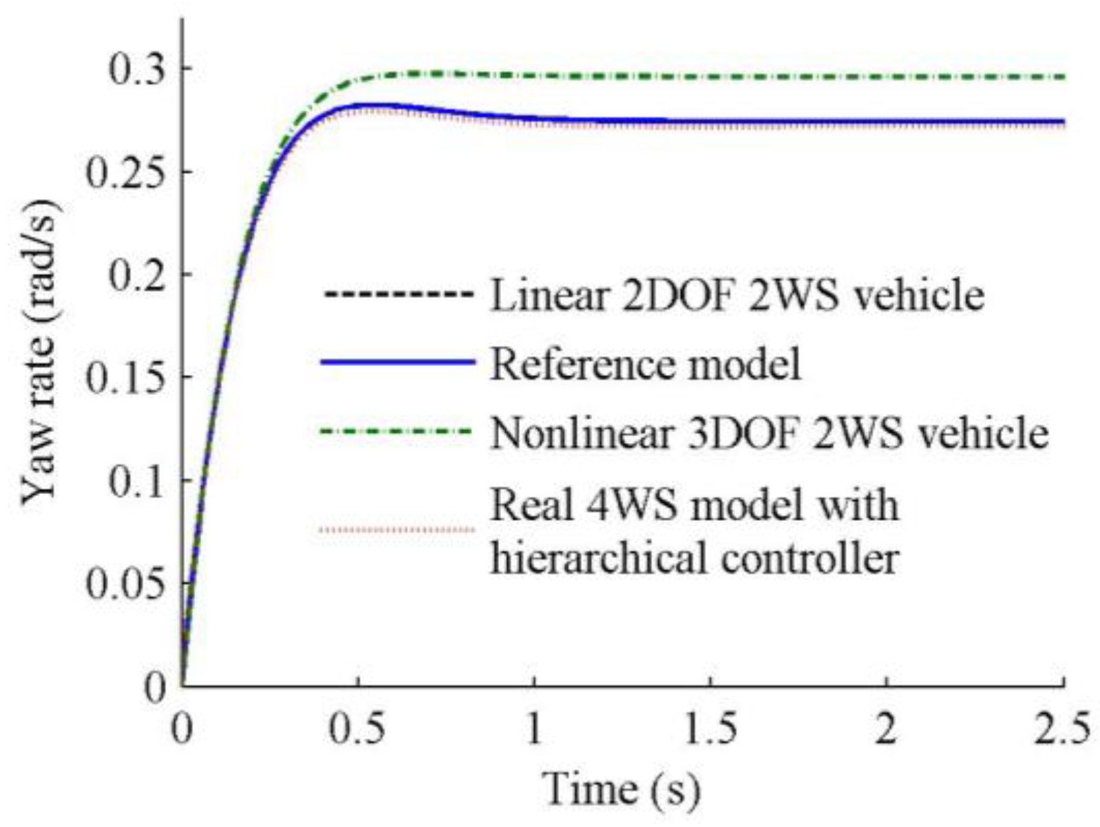
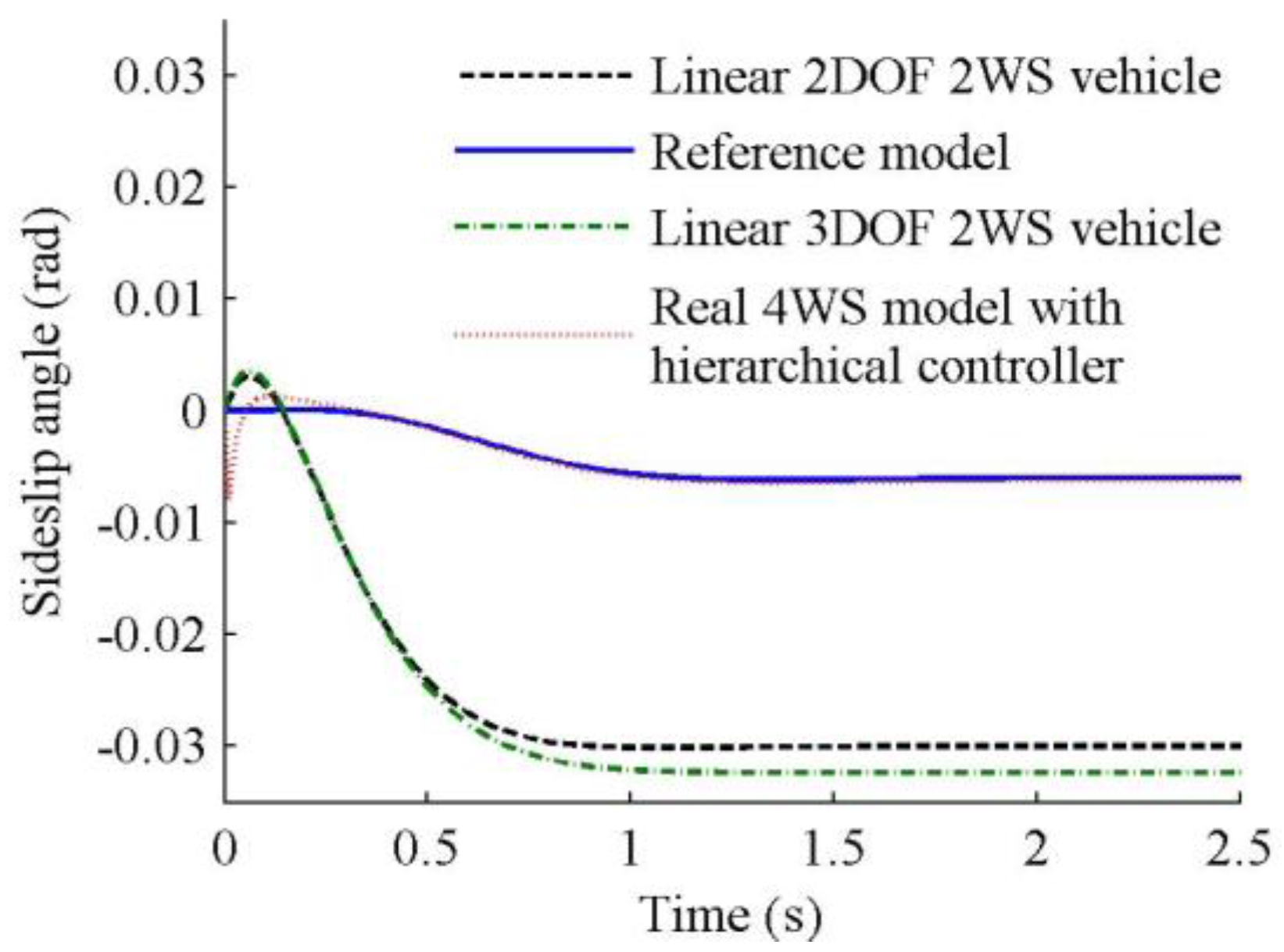
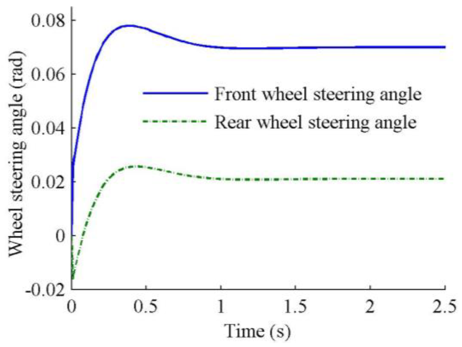
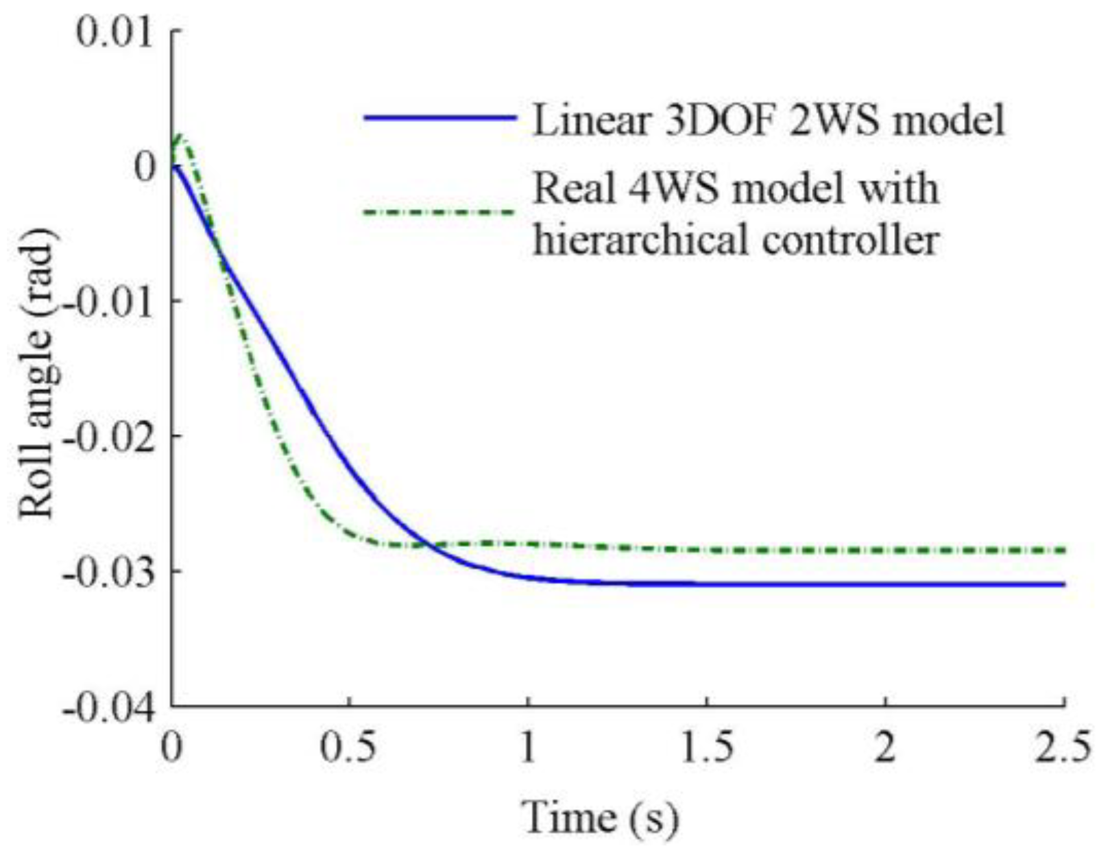
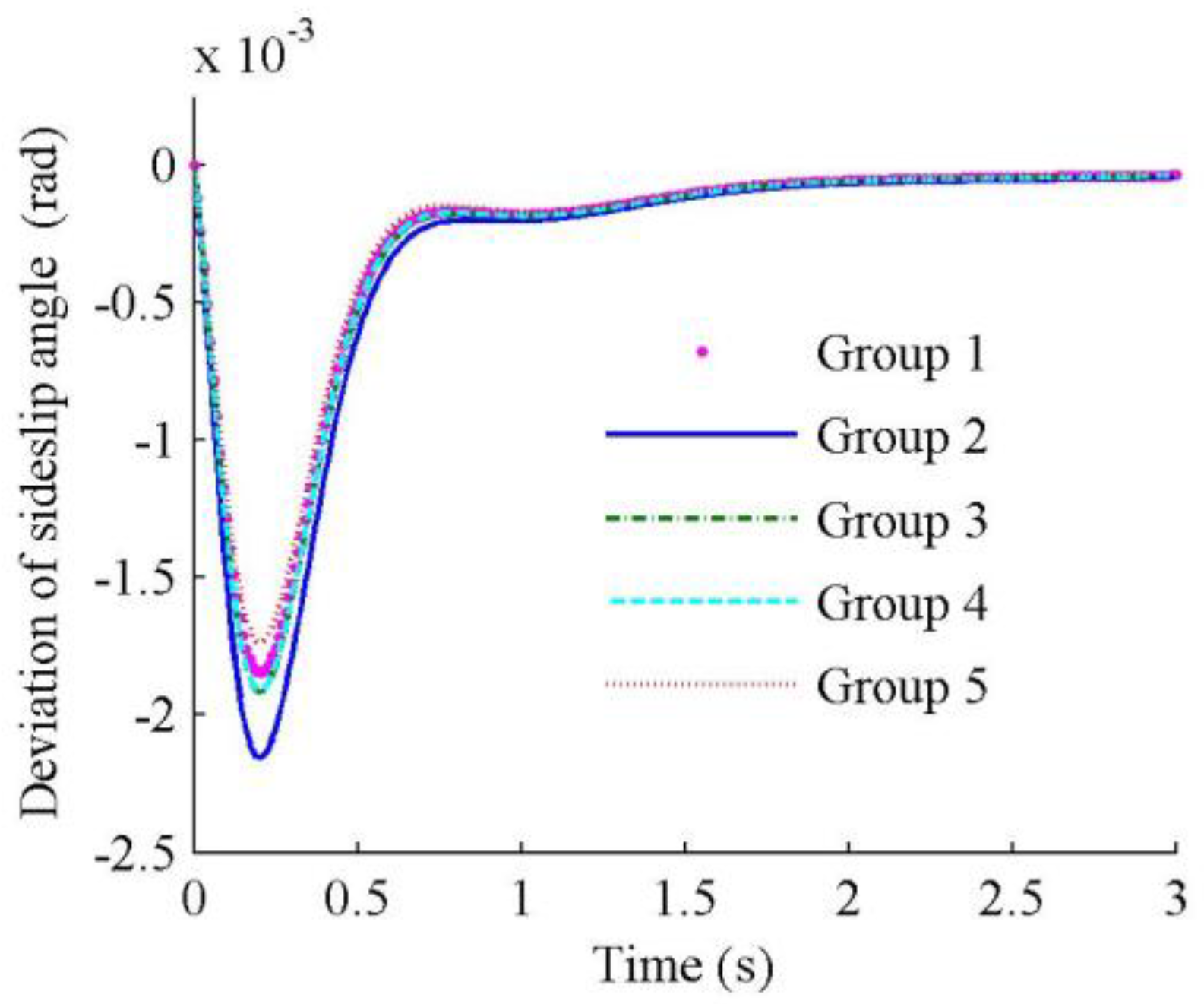
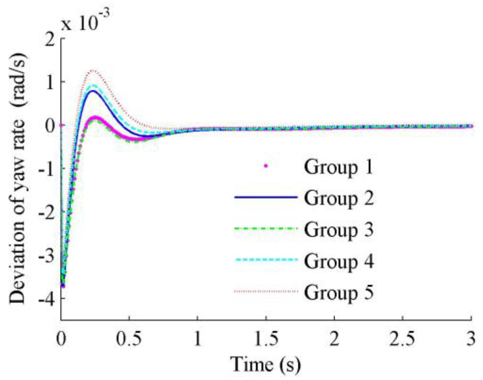
The linear 2DOF 2WS vehicle, reference model, nonlinear 3DOF 2WS vehicle, real 4WS vehicle with the hierarchical controller, and linear 2DOF 4WS vehicle with LQR controller are simulated with the same front wheel steering angle; their response curves are shown in Figure 3, Figure 4, Figure 5, Figure 6, Figure 7 and Figure 8. To investigate the robustness of the hierarchical controller system, five different groups of vehicle parameters are used in the simulation, and their deviations in yaw rate and sideslip angle from those of the real 4WS vehicle with the nominal parameters are shown in Figure 9 and Figure 10.

As shown in Figure 3 and Figure 4, the steady-state values of both the yaw rate and sideslip angle of the linear 2DOF 2WS vehicle, and those of the nonlinear 3DOF 2WS vehicle are different from each other. In particular, their steady-state values of sideslip angle are far from that of the reference model. This is because the nonlinear 3DOF 2WS vehicle considers the roll motion, and the reference model is obtained by filtering the sideslip angle of the linear 2DOF 2WS vehicle, which can also be adjusted according to the driving condition, such as the mass and speed of the vehicle. In addition, at the very beginning, the value of sideslip angle of the real 4WS vehicle with the hierarchical controller exhibits little fluctuation. However, their steady-state values of yaw rate and sideslip angle are almost exactly the same as the reference model. This is because both the partial parameters and the initial state are not the same, and the nonlinear 3DOF 4WS vehicle requires extra consideration for the roll motion.

It can be drawn from Figure 5 that front and rear wheel steering angles of the real 4WS vehicle with hierarchical controller are 0.0698 rad and 0.0215 rad, respectively, which are less than the saturation values. Further, the front and the rear wheels rotate in the same direction, thus fully meeting the requirement of the handling stability at high speed. In addition, it also indicates that although the input of the hierarchical control system is only the front wheel steering angle, the proper front and rear wheel steering angles are obtained by the hierarchical controller. Specifically, the actual front and rear steering angles come from two parts: one is the standard input achieved by the upper controller of the 4WS vehicle, the other is the corrected value obtained by the lower controller to eliminate the uncertainty influence.

Figure 6 shows that the roll angles of the nonlinear 3DOF 2WS vehicle and the real 4WS vehicle with hierarchical controller are −0.031 rad and −0.0285 rad, respectively, thus indicating that the roll angle of the rear 4WS vehicle decreases to a certain extent by adopting the hierarchical controller, and its handling stability is improved compared with the nonlinear 3DOF 2WS vehicle.

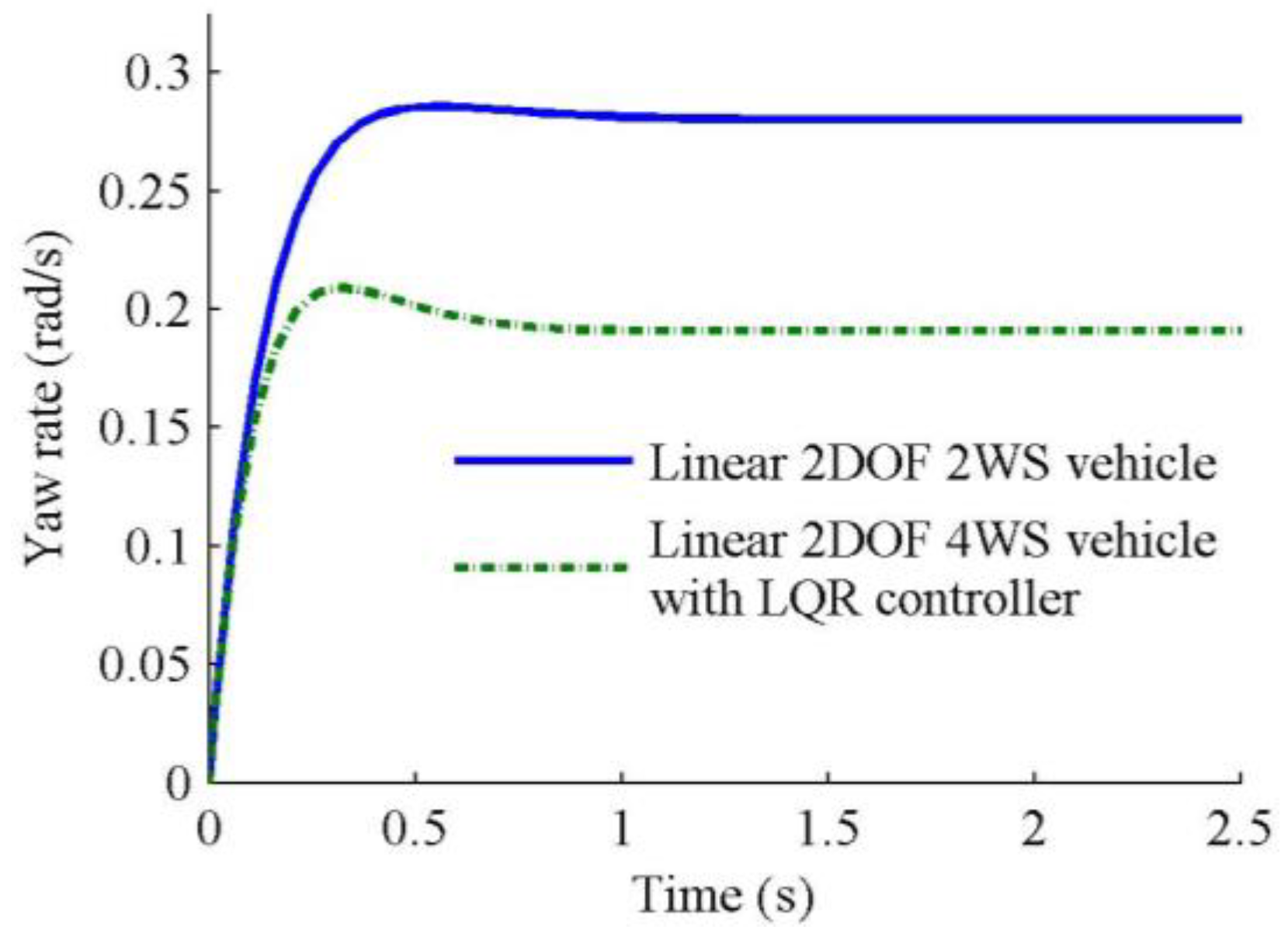
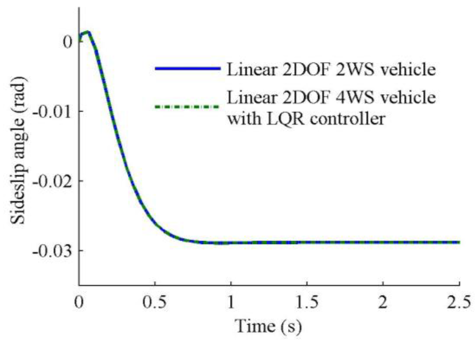
It can be seen from Figure 7 and Figure 8 that the yaw rate of the linear 2DOF 4WS vehicle with LQR controller can track that of the linear 2DOF 2WSvehicle, but the sideslip angle of the former cannot track that of the latter. Thus the upper controller of the hierarchical control strategy is effective to track both the yaw rate and sideslip angle.

As shown in Figure 9 and Figure 10, although almost all of the parameters of the real 4WS vehicle have changed, the maximum deviations in the yaw rate and sideslip angle of the real 4WS vehicle with the hierarchical controller are −3.7 × 10⁻³ rad/s and −2.16 × 10⁻³ rad, respectively, which approach 0 after approximately 1 s and 1.5 s, respectively. Hence, even if the actual 4WS vehicle is traversing with little change in these parameters, the driver will hardly feel these variations and experience no uncomfortable feeling. Obviously, the hierarchical controller demonstrates good robustness.

5. Conclusions

The realization of a new hierarchical control strategy for the nonlinear 3DOF 4WS vehicle is studied. The upper control calculates and controls the standard input for the 4WS vehicle, thus allowing the linear 2DOF 4WS vehicle to track the yaw rate and sideslip angle of the 2WS reference model. The lower control is used primarily to solve the effects of the vehicle uncertainty, and perform the appropriate amendments to yield the required performance in the real vehicle. That is, the optimal controller is applied to control the state error caused by the different initial states of the variable; subsequently, the fractional order sliding mode controller is applied to compensate for the state error caused by the uncertainty error. And the simulation results show that this hierarchical control strategy is effective for the nonlinear 3DOF 4WS vehicles.

References

1. Chen, N.; Chen, N.; Chen, Y.D. On fractional control method for four-wheel-steering vehicle. Sci. China Technol. Sci. 2009, 52, 603–609. [Google Scholar] [CrossRef]
2. Sun, C.Y.; Zhang, X.; Xi, L.H.; Tian, Y. Design of a path-tracking steering controller for autonomous vehicles. Energie 2018, 11, 1451. [Google Scholar] [CrossRef]
3. Ching, N.T.; Hormoz; Dai, V.Q.; Simic, M.; Khayyam, H.; Marzbani; Jazar, R.N. Autodriver autonomous vehicles control strategy. Procedia Comput. Sci. 2018, 126, 870–877. [Google Scholar]
4. Krishna, S.; Narayanan, S.; Ashok, S.D. Fuzzy logic based yaw stability control for active front steering of a vehicle. J. Mech. Sci. Technol. 2014, 28, 5169–5174. [Google Scholar] [CrossRef]
5. Yin, G.D.; Chen, N.; Wang, J.X.; Chen, J.-S. Robust control for 4WS vehicles considering a varying tire-road friction coeffcient. Int. J. Automot. Technol. 2010, 11, 33–40. [Google Scholar] [CrossRef]
6. Zhao, W.Z.; Qin, X.X. Study on mixed H2/H robust control strategy of four wheel steering system. Sci. China Technol. Sci. 2017, 60, 1–10. [Google Scholar] [CrossRef]
7. Li, M.; Jia, Y.; Du, J. LPV control with decoupling performance of 4WS vehicles under velocity-varying motion. IEEE Trans. Control Syst. Technol. 2014, 22, 1708–1724. [Google Scholar]
8. Chen, C.; Shu, M.; Liu, R. Virtual-point-based asymptotic tracking control of 4WS vehicles. Int. J. Control Autom. Syst. 2015, 13, 371–378. [Google Scholar] [CrossRef]
9. Mihaly, A.; Gaspar, P.; Nemeth, B. Multiple fault-tolerant in-wheel vehicle control based on high-level control reconfiguration. IFAC-PapersOnLine 2017, 50, 8606–8611. [Google Scholar]
10. Huang, D.W.; Wang, H.L.; Zhu, Z.W.; Zhang, F. Stochastic stability of four-wheel-steering system. Chaos Soliton Fractals 2007, 33, 823–828. [Google Scholar] [CrossRef]
11. Ackermann, J. Robust decoupling of car steering dynamics with arbitrary mass distribution. In Proceedings of the 1994 American Control Conference—ACC ’94, Baltimore, MD, USA, 29 June–1 July 1994; pp. 1964–1968. [Google Scholar]
12. Zhu, Z.; Du, R. Yaw Moment control strategy for four-wheel side driven EV. Autom. Control Comput. Sci. 2018, 52, 32–39. [Google Scholar] [CrossRef]
13. Shen, H.; Tan, Y.S. Vehicle handling and stability control by the cooperative control of 4WS and DYC. Mod. Phys. Lett. B. 2017, 31, 19–21. [Google Scholar] [CrossRef]
14. Hang, P.; Chen, X.; Fang, S.; Luo, F. Robust control for four-wheel-independent-steering electric vehicle with steer-by-wire system. Int. J. Automot. Technol. 2017, 18, 785–797. [Google Scholar] [CrossRef]
15. Koumboulis, F.N.; Skarpetis, M.G. Robust triangular decoupling with application to 4WS cars. IEEE Trans. Autom. Control 2000, 45, 344–352. [Google Scholar] [CrossRef]
16. Fujimoto, H.; Yamauchi, Y. Advanced motion control of electric vehicle based on lateral force observer with active steering. IEEE Int. Symp. Ind. Electron. 2010, 3627–3632. [Google Scholar]
17. Skarpetis, M.G.; Koumboulis, F.N.; Barmpokas, F.S.; Chamilothoris, G.E. Decoupling control algorithms for 4ws vehicles. In Proceedings of the IEEE International Conference on Mechatronics, Budapest, Hungary, 3–5 July 2006; pp. 499–504. [Google Scholar]
18. Chen, C.; Jia, Y.; Gao, Q.; Yu, F. Asymptotic Decoupling Control with Active Front Steering and Electronic Differentials in Four Wheel Steering Vehicles. In Proceedings of the 30th Chinese Control Conference, Yantai, China, 22–24 July 2011; pp. 111–116. [Google Scholar]
19. Li, M.X.; Jia, M.Y. Precompensation decoupling control with H∞ performance for 4WS velocity-varying vehicles. Int. J. Syst. Sci. 2016, 47, 3864–3875. [Google Scholar] [CrossRef]
20. Chen, C.; Tan, H. Steering Control of High Speed Vehicles: Dynamic Look Ahead and Yaw Rate Feedback. In Proceedings of the 37th IEEE Conference on Decision & Control, Tampa, FL, USA, 18 December1998; Volume 1, pp. 1025–1030. [Google Scholar]
21. Chen, C.; Jia, Y. Nonlinear decoupling control of four-wheel-steering vehicles with an observer. Int. J. Control Autom. Syst. 2012, 10, 697–702. [Google Scholar] [CrossRef]
22. Marino, R.; Cinili, F. Input–Output decoupling control by measurement feedback in four-wheel-steering vehicles. IEEE Trans. Control Syst. Technol. 2009, 17, 1163–1172. [Google Scholar] [CrossRef]
23. Yuhara, N.; Horiuchi, S.; Arato, Y. A robust adaptive rear wheel steering control system for handling improvement of four-wheel steering vehicles. Veh. Syst. Dyn. 1992, 20, 666–680. [Google Scholar] [CrossRef]
24. Manabe, S. A suggestion of fractional-order controller for flexible spacecraft attitude control. Nonlinear Dyn. 2002, 29, 251–268. [Google Scholar] [CrossRef]
Figure 1. Hierarchical control system.
Energies 11 02930 g001
Figure 2. Asymptotic tracking control system.
Energies 11 02930 g002
Figure 3. Curves of yaw rate.
Energies 11 02930 g003
Figure 4. Curves of sideslip angle.
Energies 11 02930 g004
Figure 5. Steering angles of vehicle wheels.
Energies 11 02930 g005
Figure 6. Roll angle curves.
Energies 11 02930 g006
Figure 7. Curves of yaw rate.
Energies 11 02930 g007
Figure 8. Curves of sideslip angle.
Energies 11 02930 g008
Figure 9. Deviation curves of yaw rate.
Energies 11 02930 g009
Figure 10. Deviation curves of sideslip angle.
Energies 11 02930 g010