An Extended Kalman Filter Approach for Accurate Instantaneous Dynamic Phasor Estimation

Abstract

This paper proposes the application of a non-linear Extended Kalman Filter (EKF) for accurate instantaneous dynamic phasor estimation. An EKF-based algorithm is proposed to better adapt to the dynamic measurement requirements and to provide real-time tracking of the fundamental harmonic components and power system frequencies. This method is evaluated using dynamic compliance tests defined in the IEEE C37.118.1-2011 synchrophasor measurement standard, providing promising results in phasor and frequency estimation, compliant with the accuracy required in the case of off-nominal frequency, amplitude and phase angle modulations, frequency ramps, and step changes in magnitude and phase angle. An important additional feature of the method is its capability for real-time detection of transient disturbances in voltage or current waveforms using the residual of the filter, which enables flagging of the estimation for suitable processing.

1. Introduction

Accurate estimation of synchrophasors of voltage and current waveforms is a key aspect of the correct operation of modern electric power systems. IEEE standard C37.118.1-2011 defines the measurement of synchrophasors under all operation conditions, specifying methods for evaluating these measurements and requirements for compliance with the standard, under both steady-state and dynamic conditions [1,2].

The traditional methods for synchrophasor estimation are based on a steady-state model that assumes phasor parameters are constant during the measurement window, but in general, power system voltage and currents are not steady-state sinusoidal waveforms, particularly during disturbances. Harmonic and other non-harmonic frequency components, step changes in magnitude and phase angle, oscillations, fast transients, and high-frequency components can be produced during electromagnetic and electromechanical transient disturbances. The estimation of phasors under these dynamic conditions may produce erroneous results as is reported in [3].

Discrete Fourier Transform (DFT)-based phasor estimation algorithms have traditionally been used because of their good performance in steady-state conditions, and they are used in many commercial phasor measurement units (PMUs), but they fail for off-nominal frequencies and under transient and dynamic conditions. Under these conditions, time-varying amplitude and phase angle models have been proposed to improve the accuracy of phasor estimation and for compliance with synchrophasor measurement standards [4,5,6,7,8,9,10,11,12].

Dynamic phasor estimation algorithms have been proposed [4,5,6], where the phasor is approximated with a Taylor polynomial expansion around the reference time. A Kalman filter was used [7,8] to estimate a dynamic phasor and its derivatives. A state-space model was used where the dynamic phasor was approximated by a kth Taylor polynomial expansion. The state-space model uses the phasor and its derivatives as the state variables and a state transition matrix obtained from the derivatives of each Taylor truncated dynamic phasor, applying the Kalman filter for estimation.

A Taylor-Kalman-Fourier filter for instantaneous estimation of oscillating phasors was proposed in [9]. The signal model was extended to the full set of harmonics, using an extended transition matrix where all harmonics are included, obtaining filters that were more robust to noise and able to estimate dynamic harmonics, providing phasor estimates free from harmonic infiltration.

A modified Taylor-Kalman filter for instantaneous phasor estimation based on an improved dynamic model was proposed in [10]. Other extensions of the Taylor-Kalman filter model have been introduced [11,12]. In [11], an output smoother was applied to improve the estimation accuracy of the method when large oscillations in amplitude and phase angle in harmonics and interharmonics affect the input waveforms. Reference [12] introduced a Taylor Extended Kalman Filter formulation that separately considers the amplitude and phase angle of the Taylor expansion. A new dynamic model was then defined that enables the reduction in the state space dimension considering different expansion orders of magnitude and phase angle, while including harmonics in the model.

A different approach from those based on the use of the synchrophasor Taylor series expansion model was proposed in [13]. An adaptive algorithm was used for phasor estimation, eliminating the effects of various transient disturbances on voltage and current waveforms. The algorithm pre-analyzes the waveforms in the observation window to detect and localize a discontinuity. The data detected before or after the singular point, excluding the transient, are used for phasor estimation.

In this paper, we propose the use of a non-linear adaptive Extended Kalman Filter (EKF) to better adapt to the dynamic requirements of power system signals. The fundamental component, the most relevant harmonic components, the dominant subsynchronous interharmonic component, and the power system frequency were used in a 13-state EKF to model the system and to estimate fundamental and harmonic phasors and the power system frequency. This method enables on-line tracking of the fundamental, harmonics, and subsynchronous interharmonic phasors and the detection of transient conditions in the input waveform using the residual of the Kalman filter.

The paper is organized as follows: Section 2 presents the main characteristics of the EKF and the signal model used in our proposal. Section 3 outlines the performance of the algorithm under off-nominal frequencies, frequency ramps, power oscillations, and step changes in magnitude and phase angle dynamic compliance tests defined in IEEE C37.118.1-2011. The obtained results are also analyzed in this section. Section 4 outlines the transient detection capability of the method and Section 5 presents the conclusions.

2. Kalman Filtering and Signal Model

2.1. Extended Kalman Filter

The Extended Kalman Filter (EKF) is a modified version of the linear Kalman filter that is applied to systems with non-linear processes and measurement equations. In each step of the recursive algorithm, the non-linear equations are linearized using a first order Taylor series to form a linear process, and then the linear Kalman filter model is applied.

The EKF defines the state transition function and the relationship between the states and the measurements by means of the nonlinear functions f and h, respectively:

$$x_{k+1}=f[x_k,k]+w_k$$

$$z_k=h[x_k,k]+v_k$$

where x_k and z_k are the state vector and the measurement at instant k, respectively; and w_k and v_k are the uncertainties introduced by the state transition and the measurement noise, both with zero mean and covariances Q_k and R_k, respectively. The nonlinear functions f and h are linearized using a first-order Taylor series as follows:

$$x_{k+1}={\Phi }_k{x}_k+w_k$$

$$z_k=H_k{x}_k+v_k$$

with

$${\Phi }_k=\frac{\partial f_i[x_k,k]}{\partial x_j}$$

$$H_k=\frac{\partial h_i[x_k,k]}{\partial x_j}$$

where f_i and h_i are the ith elements of functions f and h, respectively, and Φ_k and H_k are the state transition and the measurement matrices, respectively.

The Kalman filter is a two-step prediction-correction process. Starting with an initial estimate of the process x’_k, and its error covariance matrix P’_k, the measurement at instant k, z_k, is used to improve the estimation. A linear combination of the estimate and the measurement is chosen according to Equation (1):

$$x_k=x_k^{\prime }+K_k(z_k-H_k{x}^{\prime }{}_k)=x_k^{\prime }+K_k{\epsilon }_k$$

(1)

where x_k is the estimation update at instant k and K_k is the filter coefficient.

ε_k is the residual, defined as:

$${\epsilon }_k=z_k-H_k{x}^{\prime }{}_k$$

(2)

which represents the difference between the measurement z_k and the estimation x’_k at instant k.

The state transition matrix Φ_k is used to project the filter ahead using the measurement at instant k + 1. Kalman filter equations can be found in [14].

2.2. Signal Model

Considering the input signal as a single-phase sinusoidal with superimposed harmonic and interharmonic components:

$$x(k)={\displaystyle \sum _i^n{A}_i\sin (2\mathsf{\pi }ifk{T}_S+{\theta }_i)}+A_{ih}\sin (2\mathsf{\pi }{f}_{ih}k{T}_S+{\theta }_{ih})$$

where i is the harmonic order; A_i and θ_i are the amplitude and phase angle of each harmonic component respectively; A_ih, θ_ih, and f_ih are the amplitude, phase angle, and frequency of a dominant interharmonic component, respectively; f is the fundamental frequency; and T_s is the sampling period.

The successful application of a Kalman filter depends on the accuracy of the model used, which requires previous knowledge of the system. The lack of relevant components in the signal model may produce erroneous results in the estimation of the components of interest [11,12]. In order to estimate the dominant frequency components in a specific power system network, a DFT analysis was applied to the input signal to select the best possible state vector, which is the DFT output bins-harmonics and interharmonics-with the highest magnitudes, as well as their initialization values and error covariances.

Other proposals to obtain these dominant components in the signal to improve the accuracy of the model can be found in the literature. A compressive sensing approach was proposed in [15] to identify the most relevant components of the signal and to model them in the phasor estimation procedure. A frequency-domain decomposition of the residuals of a linear Kalman filter using the Short-Time Fourier Transform was used in [16] to obtain the dominant subsynchronous component of the signal to be included in the model of the system to achieve an accurate phasor estimation.

Fundamental and odd harmonic components from the third to the ninth are normally dominant in low-voltage supply systems and were proven in [17] as an efficient solution to model the signal. The use of a higher order model improves the accuracy of the estimation but also increases the computational complexity, so a trade-off is required between accuracy and model complexity. The presence of a dominant sub-synchronous interharmonic component close to the fundamental frequency may affect the estimation of the fundamental phasor [16]. Including this frequency component in the model of the system is necessary to obtain an accurate phasor estimate.

Another necessary and important aspect in the successful application of Kalman filters is the adequate selection of the filter parameters, the initial estimation of the state vector, and the covariance matrices, based on previous knowledge of the system to be modeled. The process and the measurement noise covariance matrices, Q_k and R_k respectively, act as tuning parameters to balance the dynamic response of the filter against the sensitivity to noise. Convergence rate and noise rejection of the filter requires a trade off against each other. The degree of stability improves as the process covariance increases and/or the noise covariance decreases [18], the filter response depending more on the ratio of these two matrices than on their specific values [19,20].

The state vector selected at instant k, x_k, is:

$$x_k={[x_1\hspace{1em}{x}_2\hspace{1em}\cdots \hspace{1em}{x}_{11}\hspace{1em}{x}_{12}\hspace{1em}{x}_{13}]}_k$$

(3)

where x₁, x₃, ..., x₉ are the in-phase components of the fundamental and the dominant harmonic components; x₂, x₄, ..., x₁₀ are the corresponding in-quadrature components; x₁₁, x₁₂ are the in-phase and in-quadrature components of the dominant sub-synchronous interharmonic component at instant k; and x₁₃ is the power system frequency. The magnitude and phase angle of each frequency component are computed using the instantaneous rectangular components considered in the model of the signal. The inclusion of the power system frequency in the state vector enables the filter parameters and the phasor to be updated with the new estimation of the frequency in each step of the recursive process, improving the accuracy of the estimation algorithm, and avoiding the need for a separate frequency estimation algorithm, as required in other previously proposed Kalman filter phasor estimation methods [16,21].

The on-line estimation of fundamental phasors and power system frequency with each new sample of the input signal allows increasing the reporting rate without decreasing the frequency resolution, which would be the case for the application DFT-based synchrophasor estimation methods.

3. Performance Analysis

The performance of the proposed phasor estimation method was evaluated using the dynamic compliance tests defined in the IEEE synchrophasor measurement standard and its amendment [1,2], for both P-class and M-class compliance. In each test, the estimated phasor at instant k is compared with the theoretical value provided as an input, computing the Total Vector Error (TVE), Frequency Error (FE), and Rate of Change of Frequency (ROCOF) Error (RFE) performance indices as measurement of the difference between the ideal values and their estimates as defined in [1].

This section presents the results obtained with the proposed method under the different dynamic tests defined in IEEE Standard C37.118.1-2011: frequency deviations, amplitude and phase angle modulations, frequency ramps, and step changes in magnitude and phase angle.

As previously mentioned in Section 2, a previous analysis of the signal in a specific power system network is required to select the dominant frequency components to be included in the state vector. To this end, the daily mean value of the fundamental and odd harmonic components from the 3rd to the 11th order and the mean square values of voltage supply measured in the specific power system network were selected as the initialization values of the state vector and its covariance matrix, respectively. We selected 50 Hz as the initial value of the power system frequency and a Q_k/R_k ratio of 10. This ratio was proven to be an efficient solution in the low-voltage distribution network in [17]. Other power system networks require a similar previous analysis to select the most adequate state vector and the initialization parameters of the Kalman filter. The sampling rate used in the simulations was 6.4 kS/s (128 samples/cycle in a 50 Hz system).

3.1. Frequency Deviation

In these tests, a constant frequency was is applied to the nominal frequency in the range of ±5 Hz for M-class or ±2 Hz for P-class compliance, with constant phase angle in steps of 0.1 Hz, as defined in [1], computing the maximum magnitudes of the three indices: TVE, FE and RFE. The maximum acceptable values of these performance indices are 1%, 0.005 Hz, and 0.01 Hz/s, respectively, for M-class compliance. According to the standard amendment [2], the values are 1%, 0.005 Hz, and 0.4 Hz/s for P-class compliance, respectively.

The test signal used in this test was [1]:

$$x(t)=X_m\cos (2\mathsf{\pi }(f_0+f_{dev})t+\varphi )$$

where X_m is the magnitude, φ is the phase angle of the fundamental component, f₀ is the nominal power system frequency, and f_dev is the frequency deviation.

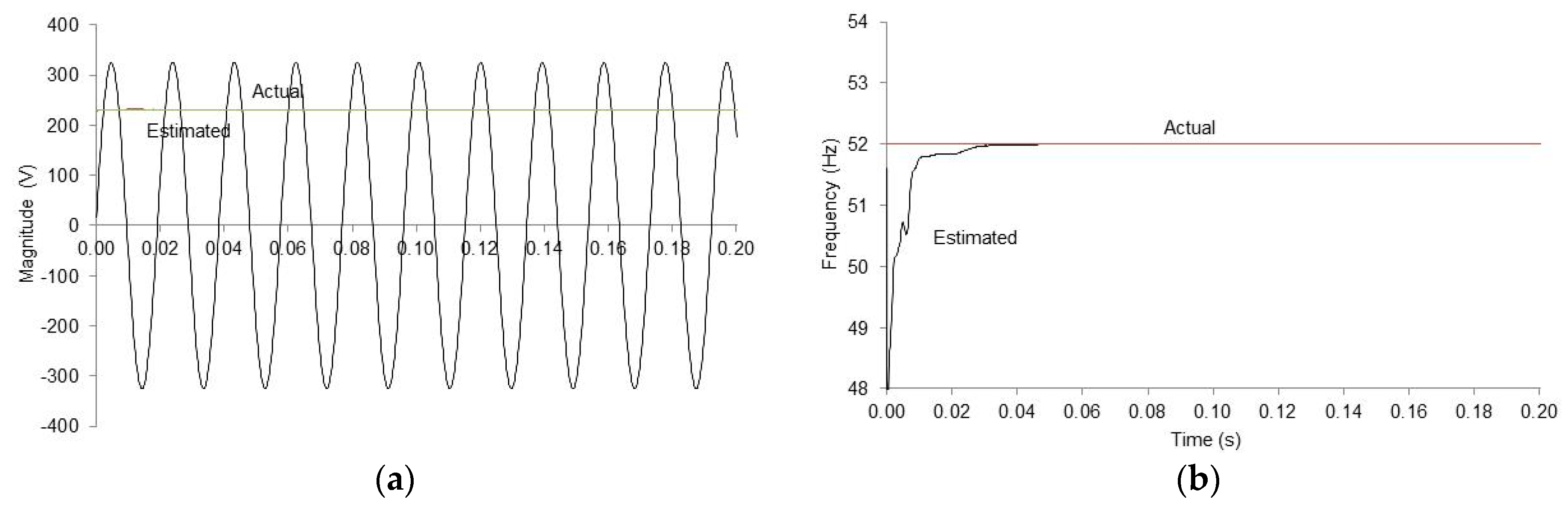
As an example of the performance of our method, Figure 1 shows the actual and the estimated magnitude and frequency in the case of a 230 V magnitude and 52 Hz voltage waveform. After a short initialization time, both the estimated magnitude and frequency quickly converged to their real values. In this case, the maximum TVE, FE, and RFE were 3.4 × 10⁻⁵%, 5.48 × 10⁻³ mHz, and 2.34 × 10⁻⁵ Hz/s respectively.

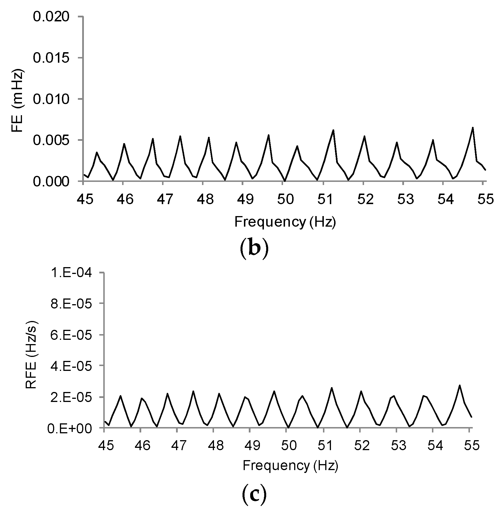
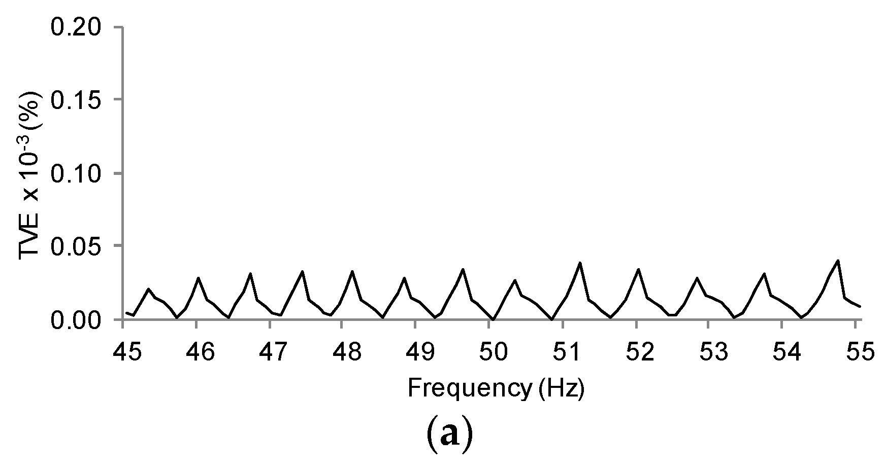
Figure 2 shows the maximum values of TVE, FE, and RFE during the five second record for each of the frequency deviation test signals. The maximum values of the three performance indices were all below the minimum requirements of the synchrophasor measurement standard for both P-class and M-class compliance.

3.2. Amplitude and Phase Angle Modulation

These tests were performed by modulating the input signal with sinusoidal signals simultaneously applied to signal magnitude and phase angle, which were used to estimate the bandwidth of the estimation algorithm. These signals are mathematically represented for a single phase as [1]:

$$x(t)=X_m[1+k_x\cos (wt)]\cos (w_{0}t+k_a\cos (wt-\mathsf{\pi }))$$

where X_m is the amplitude, w₀ is the nominal frequency, w is the modulating frequency, and k_x and k_a are the amplitude and phase angle modulation factors, respectively.

The IEEE synchrophasor measurement standard allows a maximum 3% TVE for modulating frequencies from 0.1 Hz to 5 Hz, and the maximum values of FE and RFE should be lower than 0.06 Hz and 3 Hz/s for P class compliance, respectively, and reporting rates higher than 20, and 0.3 Hz and 30 Hz/s, respectively, for M-class compliance at the same reporting rate. According to the standard, TVE, FE, and RFE indices should be measured over at least two full cycles of the signal in the different modulation tests.

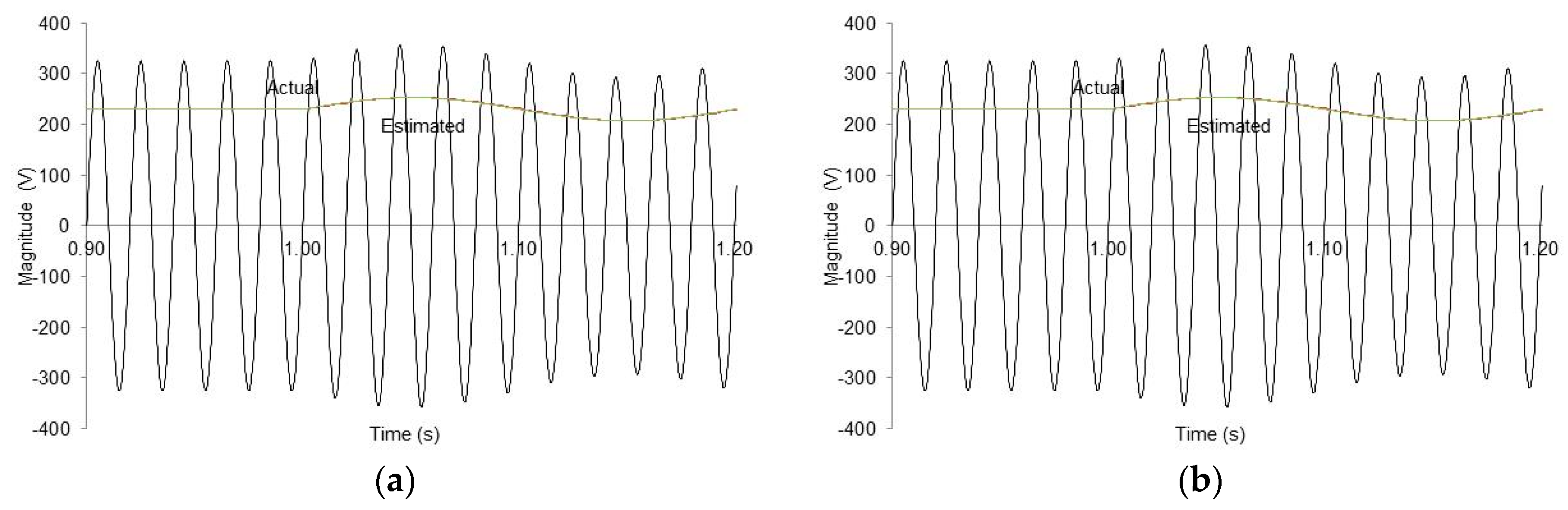
Figure 3 shows the estimated amplitude and frequency in the case of a 230 V magnitude and 50 Hz voltage waveform with a 10% magnitude, and 0.1 Hz amplitude modulation starting from 1 s of the record. As can be seen in the figure, the estimated amplitude accurately tracked the actual voltage fluctuation with minimum frequency error.

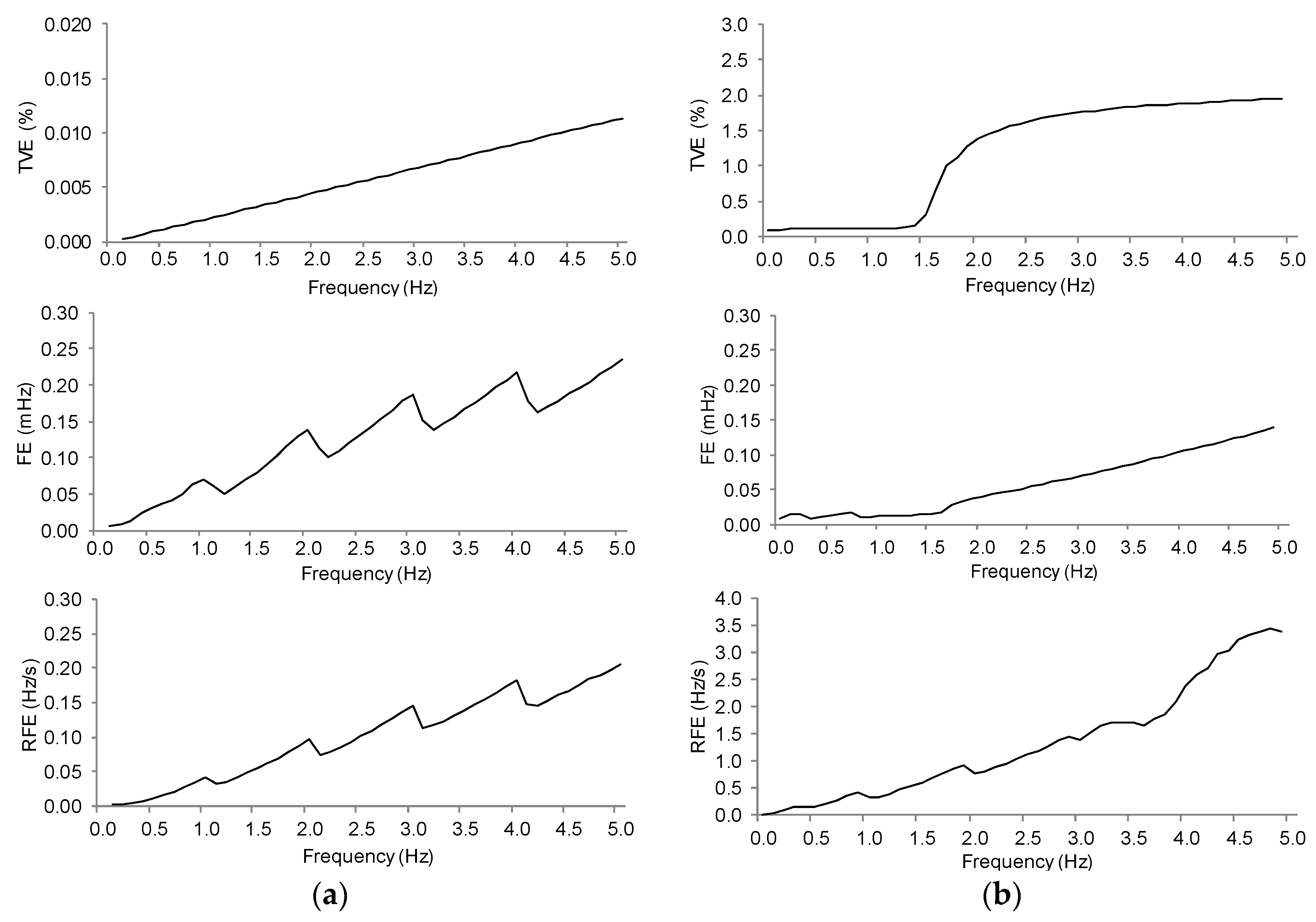
Figure 4a,b show the maximum TVE, FE, and RFE values obtained for the different amplitude and phase modulation test signals for modulation frequencies from 0.1 Hz to 5 Hz, varying in steps of 0.1 Hz and 10% amplitude and 10% phase angle modulation. From the results reported, the maximum 3% TVE criteria was satisfied under all conditions. The same applies for the measurements of maximum values of FE and RFE indices.

3.3. Frequency Ramp

According to the synchrophasor measurement standard, the performance of a measurement method should also be evaluated during frequency ramp tests. Mathematically, the input signal can be represented by:

$$x(t)=X_m\cos [w_{0}t+\mathsf{\pi }{R}_f{t}^2]$$

where X_m is the amplitude, w₀ is the nominal frequency, and R_f (=df/dt) is the frequency ramp rate in Hz/s.

According to [2], the ramp rate and the frequency range in frequency ramp tests should be ±1.0 Hz/s and ±2 Hz for P-class compliance and ±1.0 Hz/s and ±5 Hz for M-class compliance, respectively. The measurement error limit in TVE is 1% in both cases, whereas the limits are 0.01 Hz and 0.4 Hz/s (P-class), and 0.01 Hz and 0.2 Hz/s (M-class) for FE and RFE, respectively. A transition time of ±2/F_s, where F_s is the reporting rate, is allowed for TVE, FE, and RFE compliance before and after the sudden change in ROCOF occurs.

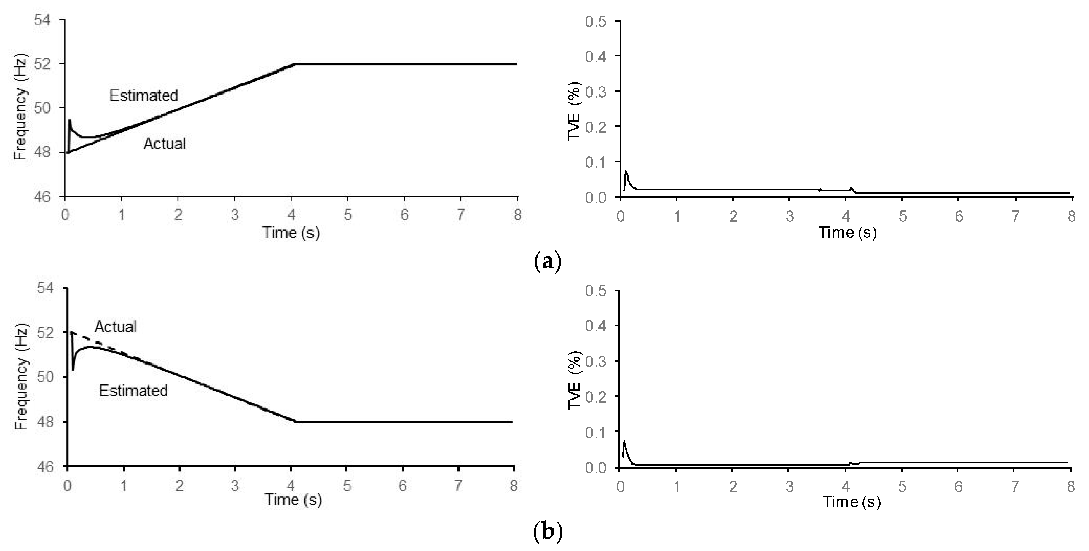
Figure 5 shows the time evolution of the frequency and TVE computed with the 13-state EKF method proposed during a positive and a negative ramp test of 1 Hz/s in the range of ±2 Hz (P-class). All results reported were obtained considering the previously mentioned exclusion intervals, with F_s = 50. With the exception of the beginning of the frequency ramp, the method presented an accurate convergence during the test. The maximum values of TVE were 0.074% and 0.071% for the positive and negative ramp test, respectively.

3.4. Step Changes in Magnitude and Phase Angle

In these tests, the test signals suddenly transitioned in the magnitude/phase angle between two steady states. The test signals were used to determine response time, delay time, and overshoot in the measurement. In our proposal, once the step change was applied, the 13-state EKF re-initialized to improve its transient response to the step change. Other proposals to improve the transient response of a Kalman filter have been previously reported [22,23,24]

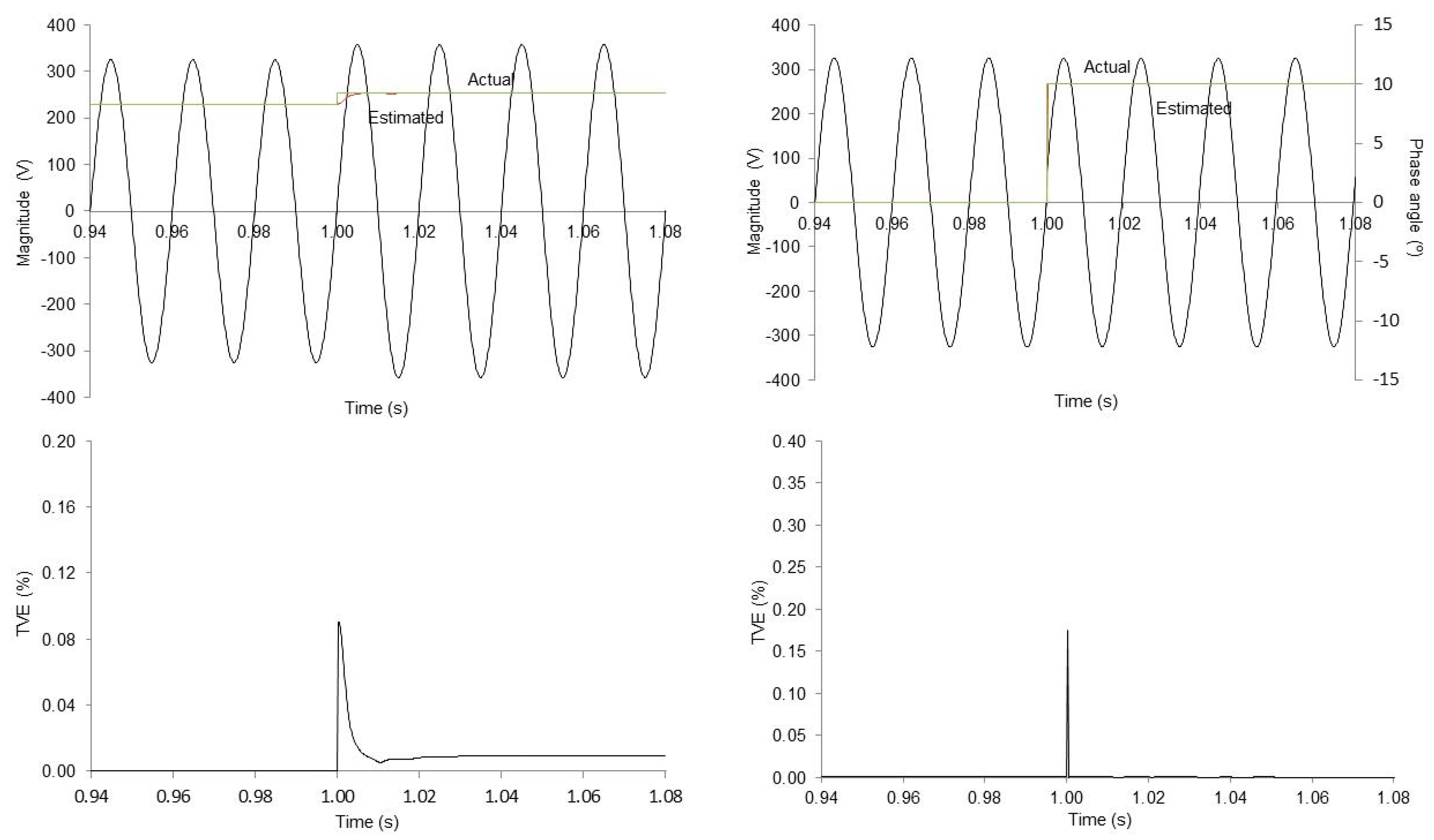
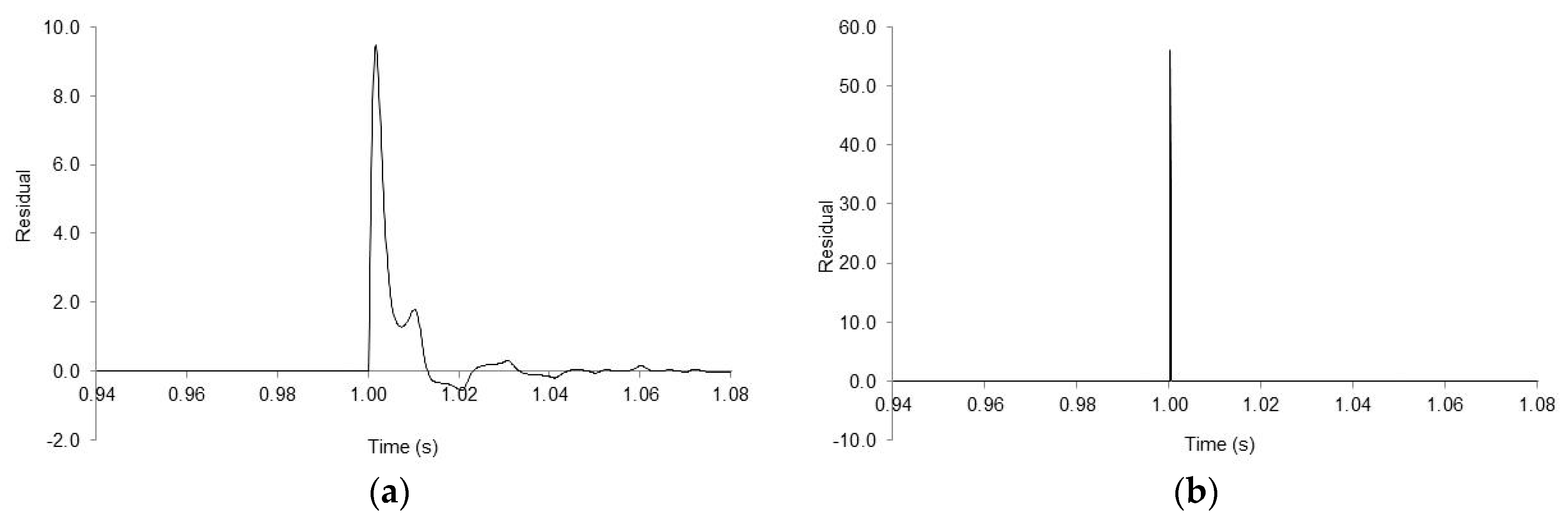
Figure 6a,b show the estimated magnitude, the residual, and TVE during a +10% step change in magnitude (k_x = 0.1) and the estimated phase angle and TVE during a +10° phase angle step change (k_a = 0.1). The method was able to accurately track these transient conditions, with the residual showing a sudden transition in its magnitude at the beginning of these changes, and the TVE always remained below the maximum 1% limit for both P-class and M-class compliance, and for step changes in magnitude and phase angle.

Table 1. Step changes in magnitude and phase angle test results.

Range (Hz)	TVE Tres (s)	FE Tres (s)	RFE Tres (s)	TVE Delay Time (s)	Overshoot (%)
+10%	0.0	0.0	0.00015	0.00031	0.524
−10%	0.0	0.0	0.00015	0.00031	0.729
+10°	0.0	0.0	0.00031	0.00015	0.035
−10°	0.0	0.0	0.00031	0.00015	0.028

presents the response time, the delay time, and the overshoots/undershoots for TVE, FE, and RFE for ±10% and ±10° step changes in magnitude and phase angle, respectively, for P-class compliance and a reporting rate F_s = 50. The maximum response time, delay time, and overshoot are defined in Tables 9 and 10 of [2]. In the case of TVE and FE, the response time with the 13-state EKF was zero because the magnitude of both indices was always below the limits defined for P-class and M-class compliance. The maximum response time for RFE (6/f₀, i.e., 0.12 s for a 50 Hz system, for the step change in magnitude and phase angle in P-class, and 14/F_s, i.e., 0.28 s for F_s = 50, for both step change tests in M-class) was not surpassed in any of the tests.

The results obtained show the high responsiveness and good estimation of step inputs of our method, with short response times and small overshoot.

4. Transient Detection

This section outlines an important additional feature of the method proposed: the real-time detection of sudden transients in the input signal using the residuals of the Kalman filter. In a Kalman filter, the residual ε_k, defined in Equation (2), reflects the difference between the actual measurement at instant k, z_k, and the predicted measurement H_kx’_k. This difference was computed in each step of the adaptive algorithm. A zero magnitude of the residual ε_k implies total agreement between the measurement and the prediction, whereas a sudden change in magnitude appears when a sudden mismatch occurs between the two, as was the case in the beginning of a transient condition in the signal under analysis. Large sudden changes in a signal produce larger magnitudes in the residuals ε_k.

The transient detection capability of the residuals depends on both the magnitude of the transient and the detection threshold selected. The detection of a transient condition enables the flagging of the estimation for its adequate processing and represents an important contribution of our method.

As an example of the capability of our method for step transient detection in the input signal, Figure 6a,b show the evolution of the residual ε_k during the +10% step change in magnitude and +10° step change in phase angle tests, respectively. A sudden change in magnitude of the residual ε_k can be observed at the beginning of the two step changes.

Reference [25] demonstrated the performance of their method in the detection of other important transient conditions in voltage or current waveforms in power systems, such as voltage dips and short interruptions, high-frequency transients, time varying harmonics and power swings, as well as the procedure for the most adequate selection of the transient detection threshold.

5. Conclusions

In this paper, we presented the application of an Extended Kalman Filter for instantaneous dynamic phasor and frequency estimation, which includes fundamental and harmonic components, compliant with the dynamic requirements of the IEEE synchrophasor measurement standards. The estimates are instantaneous and updated with each new sample of the signal under analysis. The filter parameters are adapted on-line with each new estimate of the power system frequency. The algorithm is robust against off-nominal frequencies and power swings, has accurate convergence during the frequency ramp tests, and shows high responsiveness and good estimation to step inputs, with short response times and small overshoot. Simultaneous with the estimation of the phasor magnitude and phase angle and frequency, the method can detect a step change in the input signal using the residual of the filter in real-time, which enables the flagging of the estimation for suitable processing.