A Method to Improve the Response of a Speed Loop by Using a Reduced-Order Extended Kalman Filter

Abstract

In servo systems, encoders are usually used to measure the position and speed signals of electric machines. But in a low speed range, the traditional M/T method has a larger time delay, which will cause an increase of the speed loop order and degradation of the speed loop performance. A method employed to reduce the delay of speed feedback by using a reduced-order Extended Kalman Filter (EKF) is introduced in this paper. The speed of the permanent magnet synchronous motor is estimated by the reduced-order EKF in a low speed range, which reduces the delay of speed feedback and extends the cutoff frequency of the speed loop to improve the dynamic performance of the servo system. In order to solve the issues that the traditional full-order EKF is sensitive to the inertia of the system and computationally complex, a composite load torque observer (CLTO) is proposed in this paper. The load torque and the friction torque are simultaneously observed by the CLTO. Additionally, the CLTO is used to reduce the order of the EKF, which reduces the sensitivity of EKF on inertia to enhance the robustness of the algorithm and simplifies the computational complexity. The feasibility and effectivity of the above method are verified by simulations and experiments.

1. Introduction

In recent years, the permanent magnet synchronous motor (PMSM) has been widely used in servo systems because of its high-power density, controllability, and ability to easily achieve a high-precision speed and position control. As the inner loop of position servo systems, the speed loop plays an essential role in the whole system performance. How to reduce the sampling delay of position and speed signals under the premise of ensuring accuracy is a key factor, which will affect the dynamic response and stability of the speed loop. Incremental encoders are widely used in position and speed measurement because they are accurate and easy embed into the system. However, in a low speed range, the M/T method [1] needs a large time delay to obtain more accurate speed information, which inevitably introduces a large feedback delay and reduces the dynamic performance of the speed loop. The M/T method is a method which works as follows:

• Counting the number of encoder pulses m₁ in a fixed period T_c.
• Recording the time interval ∆T of the next pulse edge after the fixed period.
• The calculated speed N_f (rpm) can be obtained as:

$$N_f=\frac{60(m_1+1)}{2\pi N(T_c+\Delta T)}$$

(1)

where N is the total number of encoder pulses per rotation.

Therefore, a large number of research has focused on velocity estimation methods based on sampled position signals only. However, due to discrete position signals and measurement noises, most linear observers cannot perform well in terms of both the steady-state performance and dynamic response [2,3,4,5]. Reference [2] proposed a velocity observer based on Phase Locked Loop (PLL), which reduces the fluctuation of steady-state speed, but its dynamic response is not significantly improved. Reference [3] proposed a linear observer based on an asynchronous pulse sampling method to improve the accuracy of steady-state measurement, but its linear gain cannot balance both steady-state and dynamic characteristics. With the development of control theory, the nonlinear observers have been extensively studied [6,7,8,9,10]. Although the nonlinear observer is used to improve the steady-state and dynamic performance, its dynamic response is not fast enough. Furthermore, its dynamic and steady-state parameters are not easy to determine. Reference [6] used the fal-function to construct a nonlinear observer. Compared with the linear observer, its steady-state characteristics are greatly improved, but the dynamic response characteristics still present a large feedback delay. Reference [7] proposed a method for constructing the acceleration observer by using a proportional-derivative (PD) controller to estimate speed, but the parameters of the PD controller are not easy to determine. Reference [8] proposed a method to construct a nonlinear velocity observer using mechanical models, but its gain parameters are higher in number and difficult to determine. At the same time, it requires too many motor parameters and the dynamic response is not significantly improved. Reference [9] proposed a position observer and a velocity estimator of a nonlinear actuator for an application in a sensorless control system for engines. The Extended Kalman Filter (EKF) is a filtering method based on model prediction, which helps to improve the response of the speed. Meanwhile, the measurement noise and process noise are considered in the EKF method, which helps to improve the steady-state performance [11,12,13,14,15,16,17,18,19,20,21,22,23,24,25]. Reference [11] constructed a third-order EKF for speed feedback, and its velocity loop has a good dynamic response, but requires precise inertia. A second-order EKF method which was constructed by using the voltage equation and mechanical equations of the motor is suggested in [12]. The q-axis current and the rotational speed of the motor are filtered together, but it requires the knowledge of many motor parameters. In [13], a fourth-order EKF is used for sensorless control by using the full model of a motor. Reference [14] constructed a fifth-order EKF to observe motor current and speed at the same time. Reference [18] proposed the unscented Kalman filter and the resilient extended Kalman filter-based sensorless direct torque control technique for permanent magnet synchronous motors. Reference [19] proposed a full-order Kalman Observer and Recursive Least Squares for online inertia identification and load torque observation. Reference [20] proposed an improved square root unscented Kalman filter for rotor speed estimation of permanent magnet synchronous motor sensorless drives. Reference [21] proposed a two-stage Kalman filter combining a robust and optimal algorithm for state and disturbance estimation. However, high-order EKFs are computationally complex and values of the covariance matrix are not easy to determine. They need more motor parameters, and they easily deteriorate or even fail to work properly when the parameters are mismatched, which limits their application.

In this paper, a reduced-order EKF is proposed to reduce the delay of speed feedback and extend the cutoff frequency of the speed loop to improve the dynamic performance of the servo system. In order to reduce the computational complexity of the traditional third-order EKF, a composite load torque observer (CLTO) is proposed to reduce the order of EKF. Additionally, the reduced-order EKF is easy to embedd in different occasions. At the same time, the load torque and the friction torque are observed together by the CLTO, which avoids the problem that the system friction coefficient is not easy to obtain in practical applications. Compared with other load observers, the CLTO with a PI controller displays a better adaptability and faster convergence. Meanwhile, the problem that full-order EKFs are sensitive to the inertia of systems can be solved by the CLTO based on the PI adaptive convergence method, which improves the robustness of the algorithm.

In this paper, the improved speed loop control strategy, the CLTO, and reduced order EKF equations are introduced in Section 2. In Section 3, the robustness of the system is analyzed. The choice of the values of the covariance matrix, Q, P₀, and R, is introduced in Section 4. Simulations and experiments are given in Section 5 and Section 6. Through the Simulink/MATLAB (9.1.0.441655 (R2016b)) and the experimental platform, the feasibility and effectivity of the above algorithm are verified by simulations and experiments. The final section presents the conclusions of this paper.

2. Speed Control Strategy Based on Filtered Speed Feedback by EKF

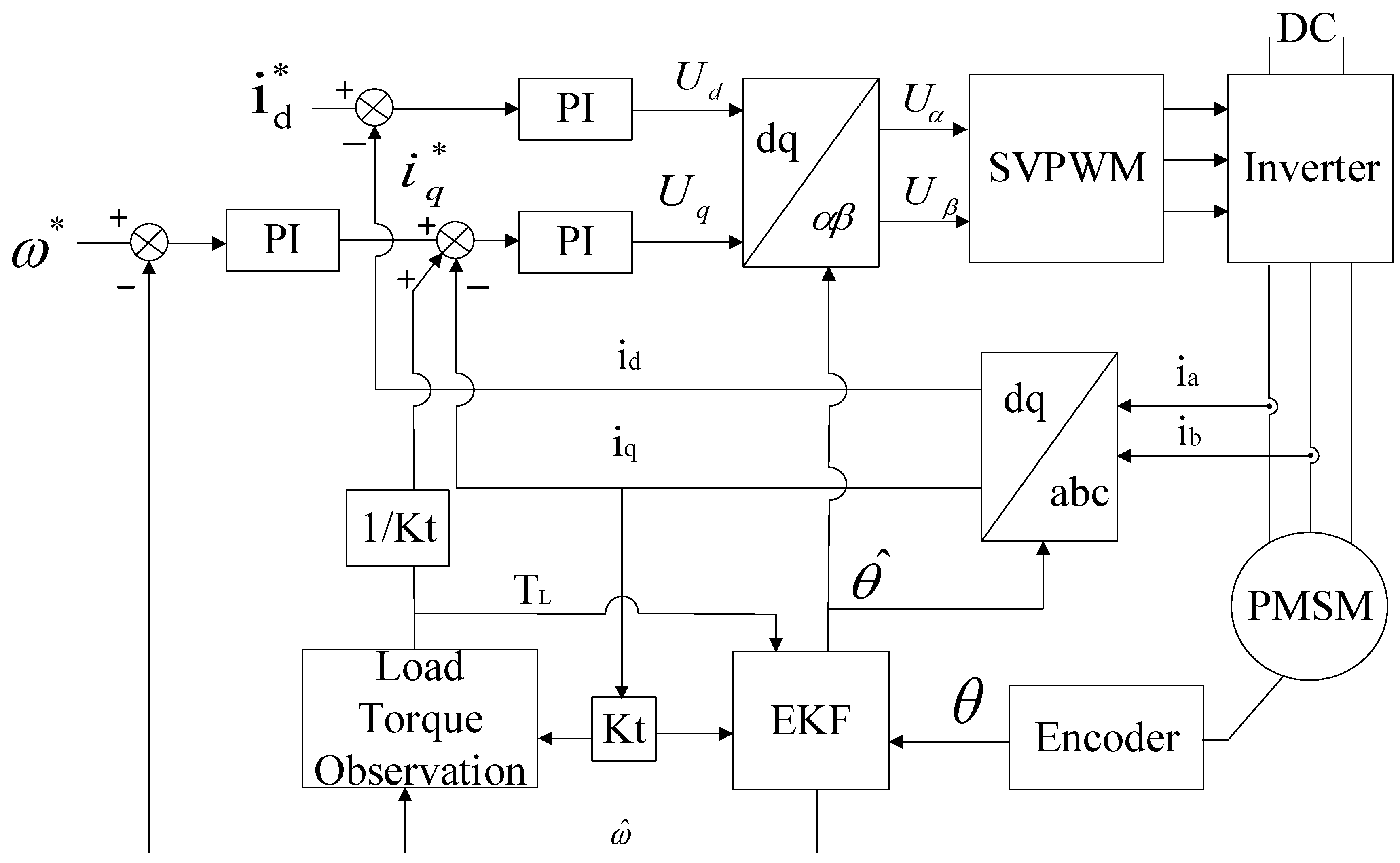
2.1. Overview of the Proposed Speed Loop Control Strategy

According to the previous analysis, in order to improve the speed loop response, the time delay of the speed feedback must be reduced. A reduced-order EKF which will be introduced in Section 2.4 is used as the speed closed-loop control, as shown in Figure 1. The control strategy is a dual closed loop control based on Field Oriented Control (FOC). The inner loop is the current loop and the outer loop is the speed loop. The observed load torque is added to the output of the speed loop as the input of the current loop. The angle filtered by the EKF is used as the coordinate transformation angle, and the filtered speed is used as speed feedback. The filtered angle is used for coordinate transformation, which reduces the discretization of the position signal and the measurement noise to the system interference. Due to observing the load torque as feedback, the system has a certain inhibitory effect on the load disturbance and it improves the system’s anti-load disturbance ability. The construction of the CLTO and the reduced-order EKF based on the mechanical model of PMSM will be introduced in the next section.

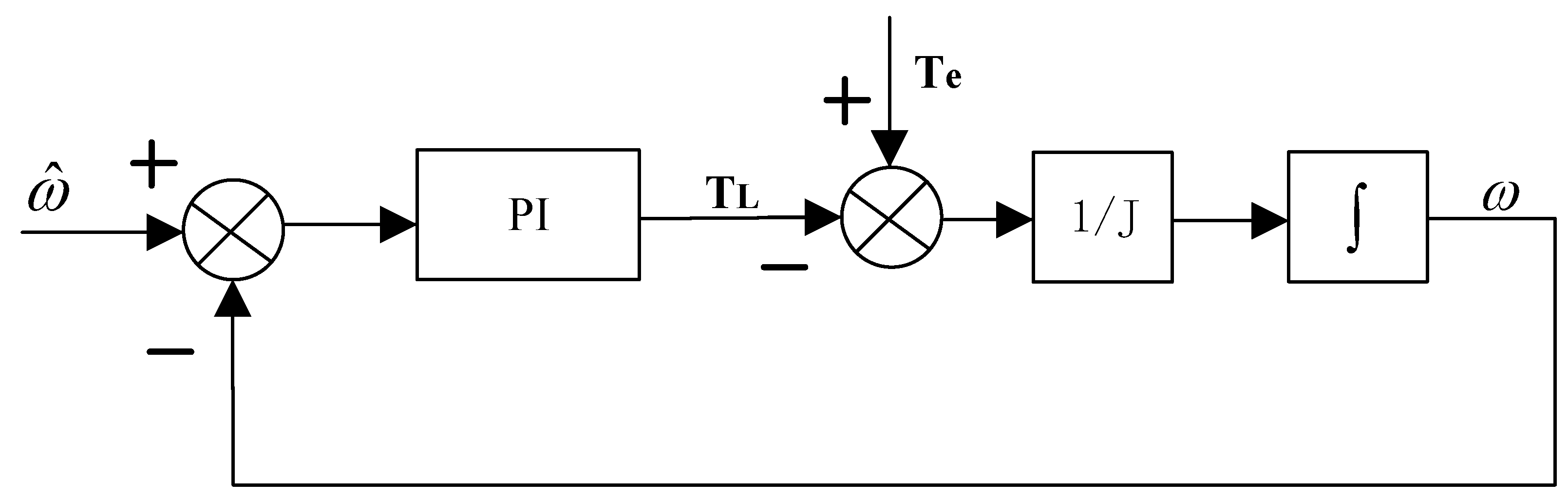
2.2. Mechanical Model of PMSM

According to mechanical equations of PMSM:

$$J\frac{d{\omega }_m}{dt}-B{\omega }_m=T_e-T_L$$

(2)

$$T_e=\frac{3}{2}{n}_p[{\phi }_f{i}_q-(L_d-L_q)i_d{i}_q]$$

(3)

where J is the inertia, B is the coefficient of friction, ${\omega }_m$ is the mechanical angel speed, T_e is the electromagnetic torque, T_L is the load torque, n_p is the number of pole pairs, ${\phi }_f$ is the permanent magnet flux linkage value, i_q is the q-axis current, i_d is the d-axis current, L_q is the q-axis inductance, and L_d is the d-axis inductance. As a surface mount PMSM, the d-q axis inductance is equal. Therefore, (3) can be simplified as follows:

$$T_e=\frac{3}{2}{n}_p{\phi }_f{i}_q$$

(4)

Considering the sampling period is T_s, it can be obtained that:

$$\{\begin{array}{l}{\theta }_k-{\theta }_{k-1}={\omega }_m{T}_s+\frac{1}{2}a{T}_s^2\\ a={\omega }_m^{\prime }=\frac{T_e-T_L-B{\omega }_m}{J}\end{array}$$

(5)

Therefore, the state equation of the system can be obtained by (2), (4), and (5), as follows:

$$\{\begin{array}{c}{\theta }^{\prime }={\omega }_m+\frac{T_s}{2J}(T_e-T_L-B{\omega }_m)\\ {\omega }_m^{\prime }=\frac{1}{J}(T_e-T_L-B{\omega }_m)\end{array}$$

(6)

2.3. Composite Load Torque Observer

State variables such as the load torque, the mechanical angle, and the speed are required in the traditional third-order EKF. In order to reduce the order of a traditional EKF, the load torque needs to be known. Therefore, a CLTO is used to estimate the load torque. The structure of the CLTO is shown in Figure 2. The speed and the electromagnetic torque are used as the input variables of the CLTO. A proportional-integral (PI) adaptive convergence method is used in CLTO. Therefore, the load torque can be obtained by the PI controller according to the error of the estimated speed and the input speed.

According to (2), (7) can be obtained as follows:

$${\widehat{T}}_L=T_L+B{\omega }_m=T_e-J\frac{d{\omega }_m}{dt}$$

(7)

where ${\widehat{T}}_L$ is the composite load torque, which includes the load torque and the friction torque. A velocity observer is constructed to estimate the composite load torque and obtain the discretization equation as:

$$\{\begin{array}{c}{\omega }_k={\omega }_{k-1}+\frac{T_s}{J}(T_{e(k)}-{\widehat{T}}_{L(k-1)})\\ {\widehat{T}}_{L(k)}=(K_p+K_i)({\widehat{\omega }}_k-{\omega }_k)+U_{k-1}\end{array}$$

(8)

where ${\widehat{\omega }}_k$ is the input speed. Here, the EKF output estimated speed is used as the input speed of the CLTO. ${\omega }_k$ is the estimated speed of the speed observer. K_p and K_i are parameters of the PI controller. $U_{k-1}$ is the integral value of $K_i$ at time k − 1. The composite load torque is calculated by the PI adaptive convergence method, which reduces the dependence of the observer on the inertia and improves the robustness of the system.

2.4. Reduced-Order EKF Equation

According to the mentioned torque observer, the traditional third-order EKF can be reduced to a second-order EKF. The mechanical angle $\theta$ and mechanical speed ${\omega }_m$ are set as state variables, the electromagnetic torque $T_e$ and the composite load torque ${\widehat{T}}_L$ are set as input variables, and the mechanical angle $\theta$ is set as the observational variable. Then, (6) can be rewritten as:

$$\left[\begin{array}{c}{\theta }^{\prime }\\ {\omega }_m^{\prime }\end{array}\right]=\left[\begin{array}{cc}0& 1\\ 0& 0\end{array}\right]\left[\begin{array}{c}\theta \\ {\omega }_m\end{array}\right]+\left[\begin{array}{cc}\frac{T_s}{2J}& -\frac{T_s}{2J}\\ \frac{1}{J}& -\frac{1}{J}\end{array}\right]\left[\begin{array}{c}{T}_e\\ {\widehat{T}}_L\end{array}\right]$$

(9)

Discretizing (9) by the Euler method, (10) can be obtained:

$$\{\begin{array}{c}{x}_k=A_{k-1}{x}_{k-1}+B_{k-1}{u}_{k-1}\\ y_k=H_k{x}_k\end{array}$$

(10)

Considering the prosses noise is ω and measurement noise is v, (10) can be rewritten as:

$$\{\begin{array}{c}{x}_k=A_{k-1}{x}_{k-1}+B_{k-1}{u}_{k-1}+w_{k-1}\\ y_k=H_k{x}_k+v_k\end{array}$$

(11)

where $A=\left[\begin{array}{cc}1& T_s\\ 0& 1\end{array}\right]$, $B=\left[\begin{array}{cc}\frac{T_s^2}{2J}& -\frac{T_s^2}{2J}\\ \frac{T_s}{J}& -\frac{T_s}{J}\end{array}\right]$, $x={\left[\begin{array}{cc}\theta & {\omega }_m\end{array}\right]}^T$, $u={\left[\begin{array}{cc}{T}_e& {\widehat{T}}_L\end{array}\right]}^T$, $y=\theta$, $H=\left[\begin{array}{cc}1& 0\end{array}\right]$, and Q and R are the covariance matrices of prosses noise and measurement noise, respectively, which can be expressed as:

$$\{\begin{array}{c}Q=\mathrm{cov}(w)=\left[\begin{array}{cc}{q}_0& 0\\ 0& q_1\end{array}\right]\\ R=\mathrm{cov}(v)=r\end{array}$$

(12)

The recursive progress of the reduced-order EKF can be separated by three steps:

• Calculating the load torque using the load observer ${\widehat{T}}_{L(k)}$.
• State variables prediction and Kalman gain calculation:

  $${\tilde{x}}_{k+1}=A{\tilde{x}}_k+B{u}_k$$

  (13)

  $${\tilde{P}}_{k+1}=A{\widehat{P}}_k{A}^T+Q$$

  (14)

  $$K_{k+1}=\tilde{P}{H}^T{(H\tilde{P}{H}^T+R)}^{-1}$$

  (15)
• Calculating the optimal estimate values and update matrix:

  $${\tilde{x}}_{k+1}={\tilde{x}}_k+K_{k+1}(y_k-H{\tilde{x}}_k)$$

  (16)

$${\widehat{P}}_{k+1}=(I-K_{k+1}H){\tilde{P}}_k$$

(17)

There are a lot of matrix operations in the EKF method. The third-order matrix operations are simplified by the reduced-order EKF, which reduces the computational complexity. Meanwhile, the EKF is a filter method based on a model which is sensitive to the inertia of the system. However, the problem can be suppressed by the CLTO, which will be discussed in the next section.

3. Robustness Analysis

Since the system adopts a new control strategy, we need to discuss the robustness of the system. Assuming the inertia input error is ∆J at time k, and the time k − 1 data are all correct values, then the changed inertia can be obtained as follows:

$$\tilde{J}=J+\Delta J=\alpha J$$

(18)

where α is the coefficient of the inertia error.

In this approach, $\tilde{\omega }$ is recorded as the estimated speed and ${\tilde{T}}_L$ as the estimated load torque obtained from the CLTO after the inertia is changed. Then, the calculated values from (8) at time k are as follows:

$${\omega }_k={\omega }_{k-1}+\frac{T_s}{J}(T_{e(k-1)}-{\widehat{T}}_{L(k-1)})$$

(19)

$${\tilde{\omega }}_k={\omega }_{k-1}+\frac{T_s}{\alpha J}(T_{e(k-1)}-{\widehat{T}}_{L(k-1)})$$

(20)

According to (19) and (20), the speed estimation error due to the inertia error is obtained as:

$$\Delta {\omega }_k={\tilde{\omega }}_k-{\omega }_k={\beta }_{k-1}(\frac{1}{\alpha }-1)$$

(21)

where ${\beta }_{k-1}=\frac{T_s}{J}(T_{e(k-1)}-{\widehat{T}}_{L(k-1)})$.

Also, the observed load torque using the PI controller from (8) can be expressed as:

$${\widehat{T}}_{L(k)}=(K_p+K_i)({\widehat{\omega }}_k-{\omega }_k)+U_{k-1}$$

(22)

$${\tilde{T}}_{L(k)}=(K_p+K_i)({\widehat{\omega }}_k-{\tilde{\omega }}_k)+U_{k-1}$$

(23)

According to (22) and (23), the torque estimation error due to the inertia error can be obtained as:

$$\Delta T_{L(k)}={\tilde{T}}_{L(k)}-{\widehat{T}}_{L(k)}=(K_p+K_i){\beta }_{k-1}(1-\frac{1}{\alpha })$$

(24)

The result of load torque is then incorporated into (13) to calculate the predicted speed of EKF. Here, it declares that ${\widehat{\omega }}_{k+1}$ as the predicted speed of EKF using the correct inertia J, with ${\overline{\omega }}_{k+1}$ as the predicted speed of EKF using the changed inertia and the uncorrected load torque ${\tilde{T}}_{L(k)}$, and ${\stackrel{⌣}{\omega }}_{k+1}$ as the predicted speed of EKF using the changed inertia and the corrected load torque ${\tilde{T}}_{L(k)}$, respectively. So:

$${\widehat{\omega }}_{k+1}={\widehat{\omega }}_k+\frac{T_s}{J}({\mathrm{T}}_{e(k)}-{\widehat{T}}_{L(k)})$$

(25)

$${\overline{\omega }}_{k+1}={\widehat{\omega }}_k+\frac{T_s}{\alpha J}({\mathrm{T}}_{e(k)}-{\widehat{T}}_{L(k)})$$

(26)

$${\stackrel{⌣}{\omega }}_{k+1}={\widehat{\omega }}_k+\frac{T_s}{\alpha J}({\mathrm{T}}_{e(k)}-{\tilde{T}}_{L(k)})$$

(27)

Then, the predicted speed error caused by the inertia error can be obtained from (25), (26), and (27) as:

$$\Delta {\overline{\omega }}_{k+1}={\overline{\omega }}_{k+1}-{\widehat{\omega }}_{k+1}={\beta }_k(\frac{1}{\alpha }-1)$$

(28)

$$\Delta {\stackrel{⌣}{\omega }}_{k+1}={\stackrel{⌣}{\omega }}_{k+1}-{\widehat{\omega }}_{k+1}={\beta }_k(\frac{1}{\alpha }-1)+\frac{T_s}{\alpha J}\Delta T_{L(k)}$$

(29)

Considering ${\beta }_k$ is approximately equal to ${\beta }_{k-1}$, (29) can be rewritten as:

$$\Delta {\stackrel{⌣}{\omega }}_{k+1}=k\Delta {\overline{\omega }}_{k+1}$$

(30)

where $k=(1-\frac{({\mathrm{K}}_p+{\mathrm{K}}_i){\mathrm{T}}_s}{\alpha J})$.

According to (30), the predicted speed error of EKF using the corrected load torque is reduced by k times compared to the uncorrected predicted speed error. From this, it can be seen that appropriately increasing the PI parameter values of the load observer helps to reduce the speed estimation error due to the inertia error. However, when the parameter values of the PI controller are too large, the steady-state fluctuation of the observed load torque will increase. So, it needs to compromise the choice of the PI parameter. It is shown that the load observer using the PI convergence method can reduce the dependence of the system on the inertia and improve the robustness of the system.

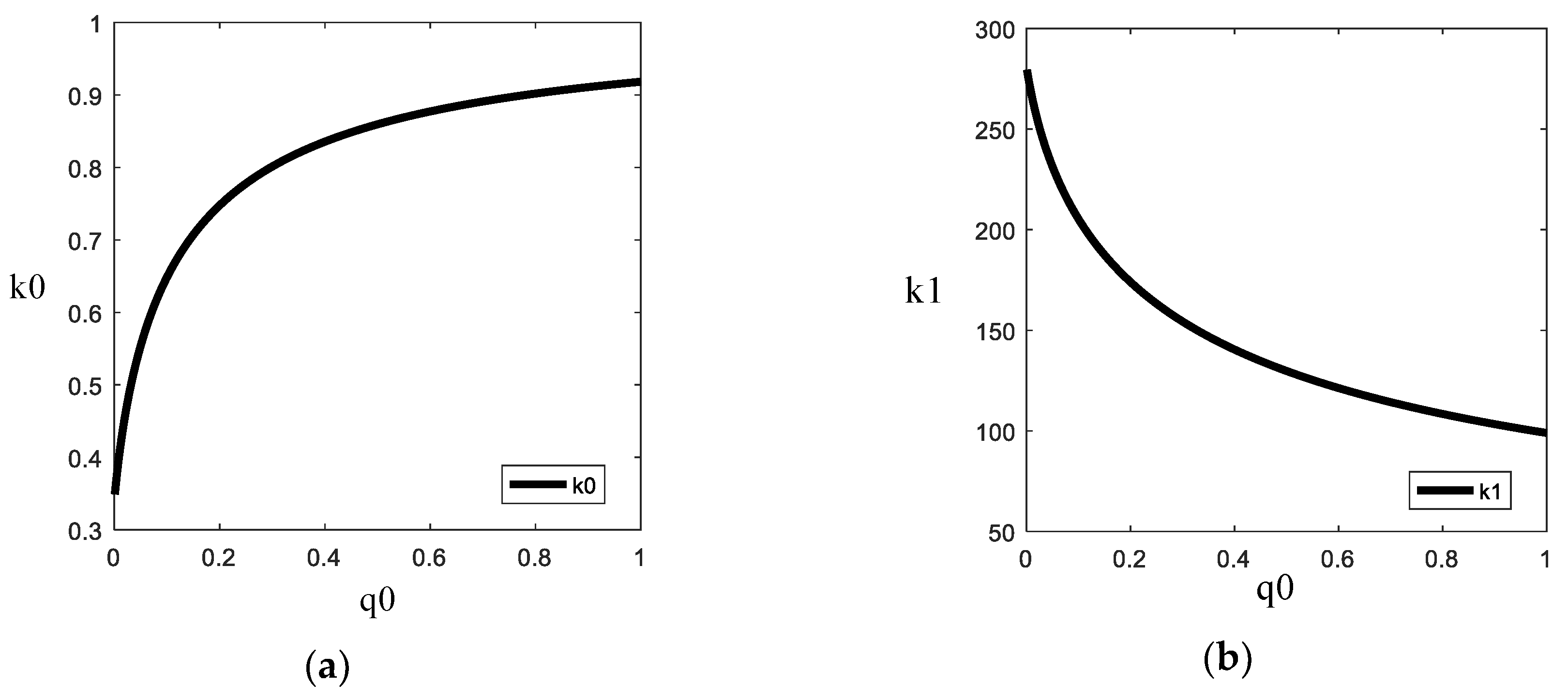
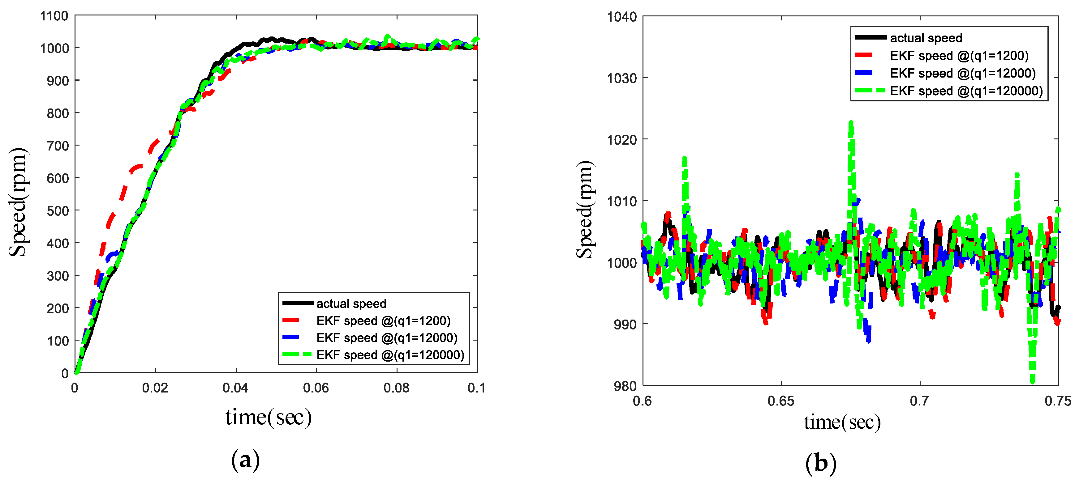
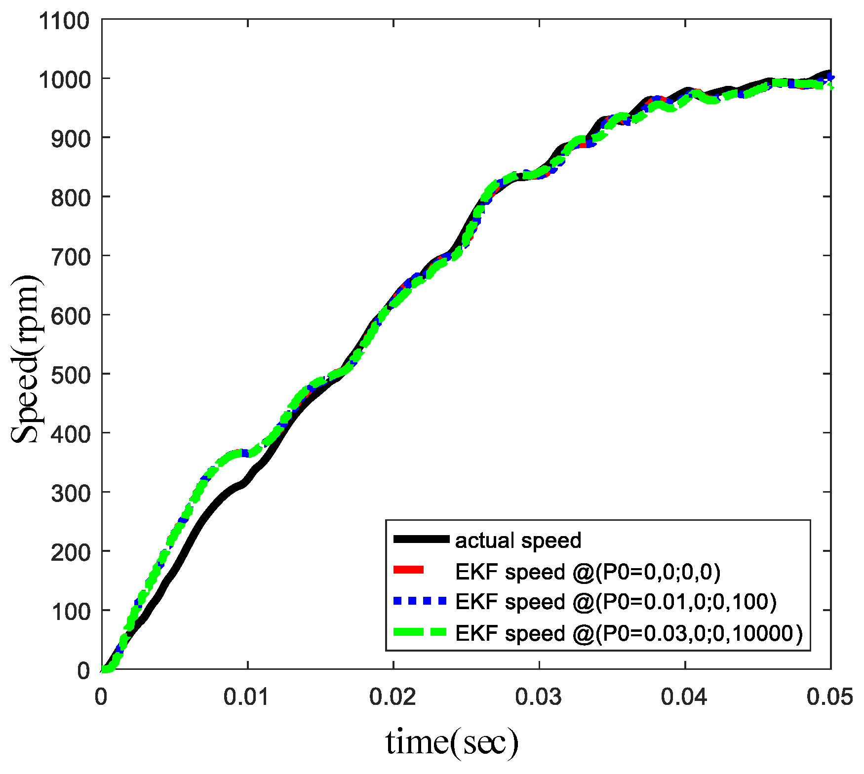
4. Design and Tuning of Q and R

A critical point during the design of EKF is the choice of the elements of the covariance matrix Q, R and the initial values of the covariance matrix P₀, which will affect the performance and the convergence [13]. In this paper, values of the covariance matrixes are obtained by trials according to the requirement of the actual system.

Matrix Q is related to the process noise. Increasing Q would indicate the presence of either heavy process noise or increased parameter uncertainty. As shown in Figure 3, increasing the value of q₀ will cause the value of k₀ to be increased and the value of k₁ to be decreased; where k₀ is the element of gain matrix K which is related to the angle error correction. The k₁ is the element of gain matrix K which is related to the speed error correction. Furthermore, as shown in Figure 4, increasing the value of q₁ will cause both the value of k₀ and the value of k₁ to be increased. Moreover, the value of k₁ is a major factor affecting the loop performance. It can be seen from Figure 5 and Figure 6 that when the value of q₀ decreases or the value of q₁ increases, it will cause the value of k₁ to be increased. This leads to an improvement in the dynamic performance of the loop, but a large steady-state fluctuation. On the other hand, matrix R is related to measurement noise. Increasing the value of the element of matrix R means the measurements are affected by noise and thus they are of little confidence. Increasing the value of r will cause both the value of k₀ and the value of k₁ to be decreased. When the values of the gain matrix K decrease, the system correction weight decreases and the state performance of the system is improved. Therefore, the comprehensive consideration has been chosen as:

$$\{\begin{array}{c}Q=\left[\begin{array}{cc}0.1& 0\\ 0& 12000\end{array}\right]\\ R=\mathrm{r}=0.1\end{array}$$

(31)

As mentioned before, it can be seen from Figure 7 that the initial value of the covariance matrix P₀ has a slightly influence on the loop performance. So, the initial value of the covariance matrix P₀ is selected as:

$$P_0=\left[\begin{array}{cc}0& 0\\ 0& 0\end{array}\right]$$

(32)

From the above results, the mentioned algorithm can work stably within a large range of parameters.

This is due to the actual position feedback of the encoder, so that the filtered speed can be kept within a reasonable range. Therefore, the EKF algorithm relying on position feedback has a good stability and convergence. It is verified that the above algorithm is working properly within, but is not limited to, this range of parameters:

$$\{\begin{array}{c}{q}_0\in [1\times {10}^{-4},1]\\ q_1\in [4000,60000]\\ r\in [0.01,1]\end{array}$$

(33)

5. Simulation and Analysis

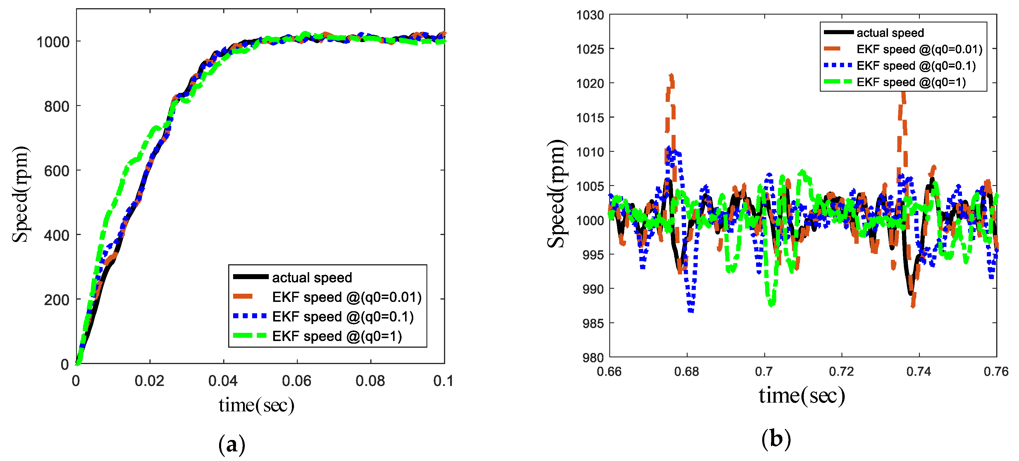
5.1. Step Excitation Simulation

After the theoretical and robustness analysis, a simulation system was built by Simulink/MATLAB. Parameters of PMSM and PI parameters of the torque observer used in simulations and experiments are shown in

Table 1. Parameters of PMSM and PI parameters of the torque observer.

Parameters	Values
Stator resister R (Ω)	1.86
Stator inductance L (mH)	2.8
Pole-pairs number	4
J (kg m2)	2.45 × 10−4
ϕf (Wb)	0.109
Kp	0.03
Ki	0.005
Ts (ms)	0.25
Encoder (1/rev)	10000

. The sampling time is selected depending on the control period of the speed loop and the current loop. Generally speaking, the control frequency of the current loop is about 12 kHz, which is an empirical value. In practical applications, the requirement of the power module in a hardware circuit and the current harmonic waves of the motor should be considered. Taking the Intelligent Power Module (FSBB30CH60F) as an example, the switching frequency is up to 20 kHz. Considering the need to minimize current harmonics and switching losses, the current loop control frequency chosen is 12 kHz. Since the mechanical response speed of the motor is much smaller than the electrical response speed, the control frequency of the speed loop selected is 4 kHz. Moreover, the sampling frequency of speed feedback and the control frequency of the speed loop are consistent for easy control. Therefore, the sampling time selected is 0.25 ms.

Figure 8 shows the simulation result of 1000 rpm step excitation. From the result, it can be seen that the delay between the estimated speed by a reduced-order EKF and the actual speed is smaller than the delay between the speed calculated by an encoder and the actual speed. This shows that the speed loop which estimated speed by the reduced-order EKF has a faster step response. Therefore, this improved method is likely to follow changes quickly when a set speed is changed rapidly. Thus, the improved method extends the cutoff frequency of the speed loop to improve the dynamic performance of the servo system. In the initial stage of the simulation, the EKF estimated the speed curve slightly ahead of the real speed curve, which is caused by the dynamic response of the CLTO not being fast enough. When the speed reaches the set value, there is no significant difference between the steady-state speed of the two methods.

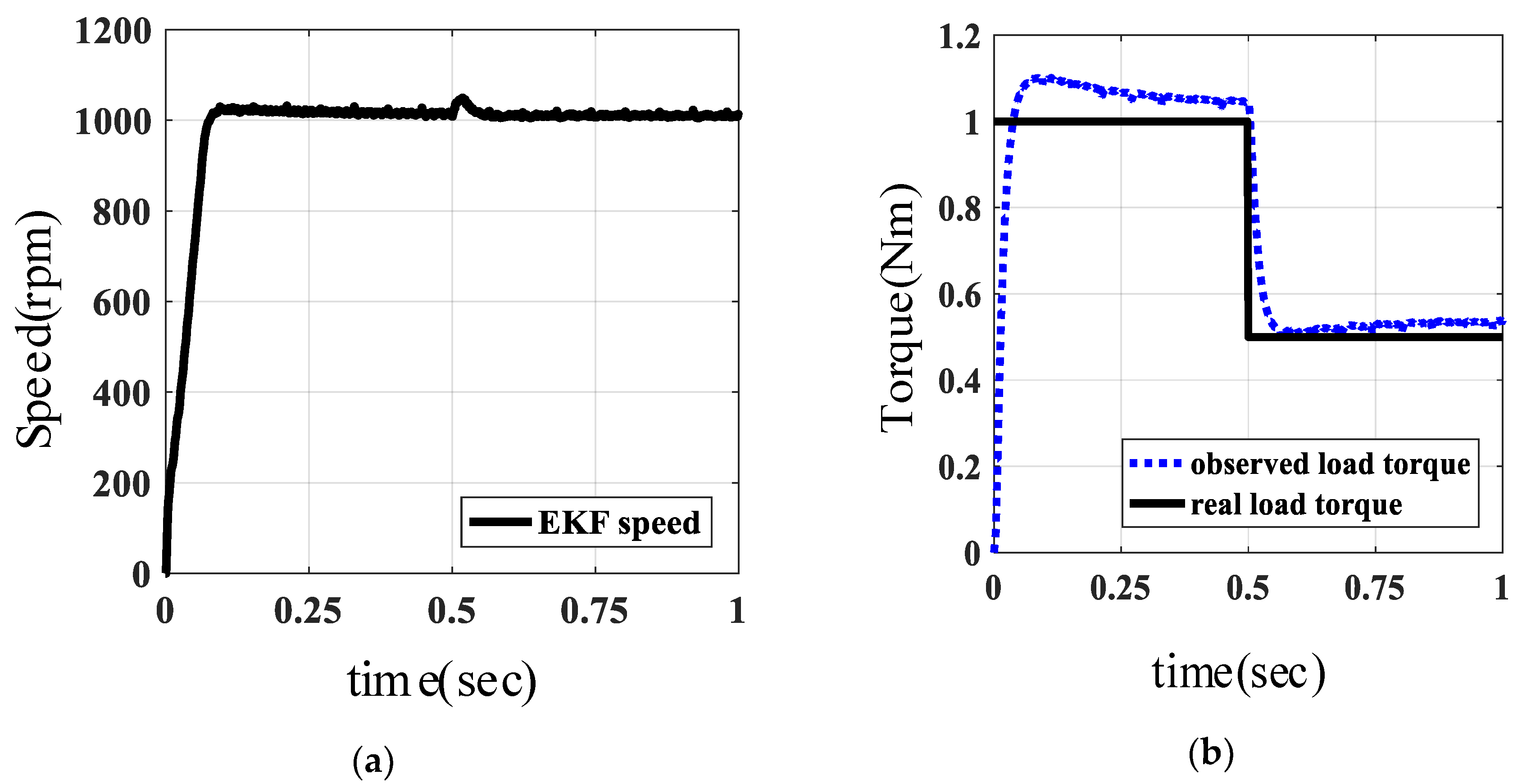
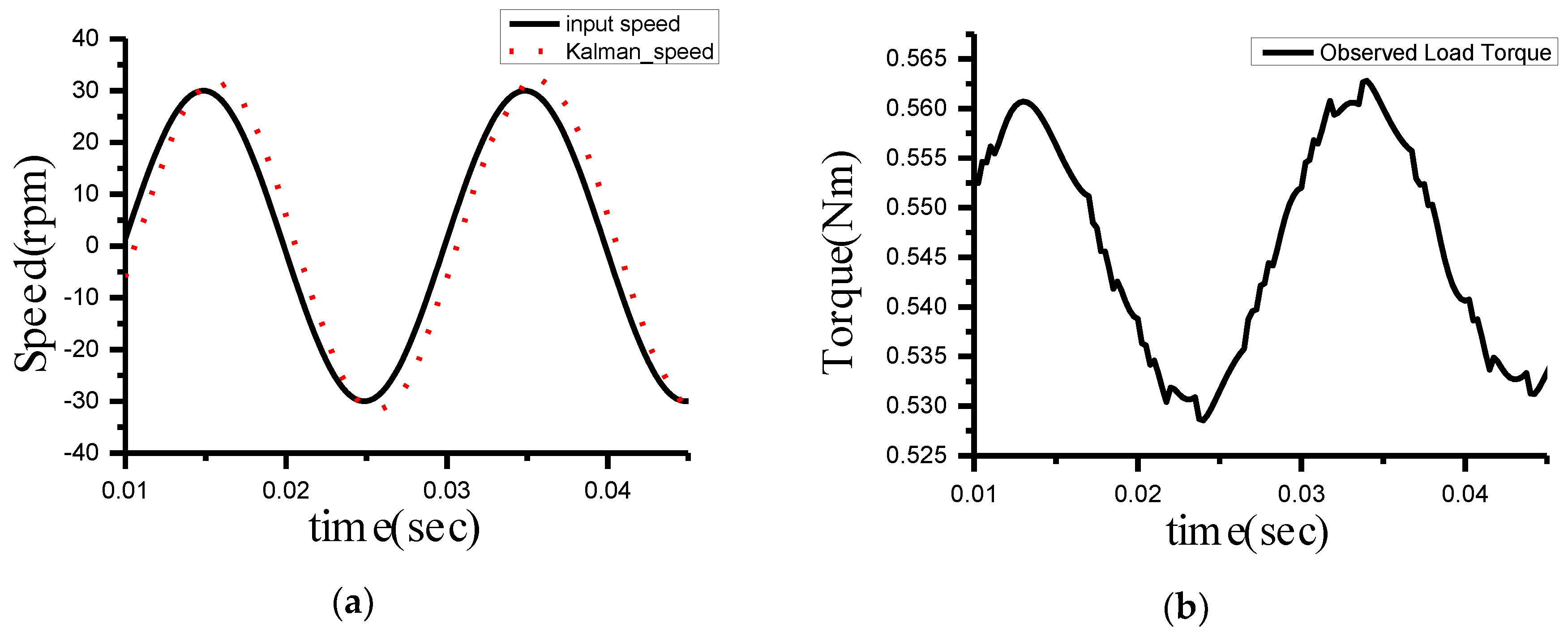
5.2. Load Torque Simulation

In order to verify the dynamic performance of the above algorithm when the load changes, the situation when the load torque increases and the load torque decreases during motor operation is simulated, as shown in Figure 9 and Figure 10. When the load torque suddenly increases or decreases at 0.5 s, the speed will drop or overshoot slightly, but it will return to the set speed very quickly in a short time, indicating that the system is highly resistant to load disturbance. This is because the CLTO has a certain negative feedback effect when the load changes so that the system can remain stable when the load changes. The load torque estimated by the load observer contains the friction torque and the load torque, so it is slightly larger than the actual load torque value and will increase as the speed increases.

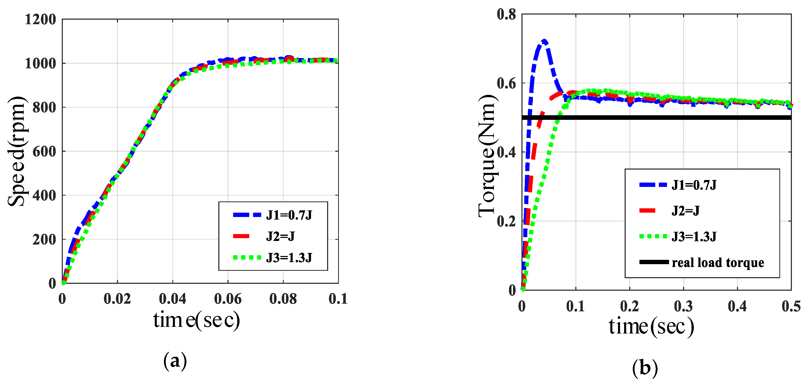
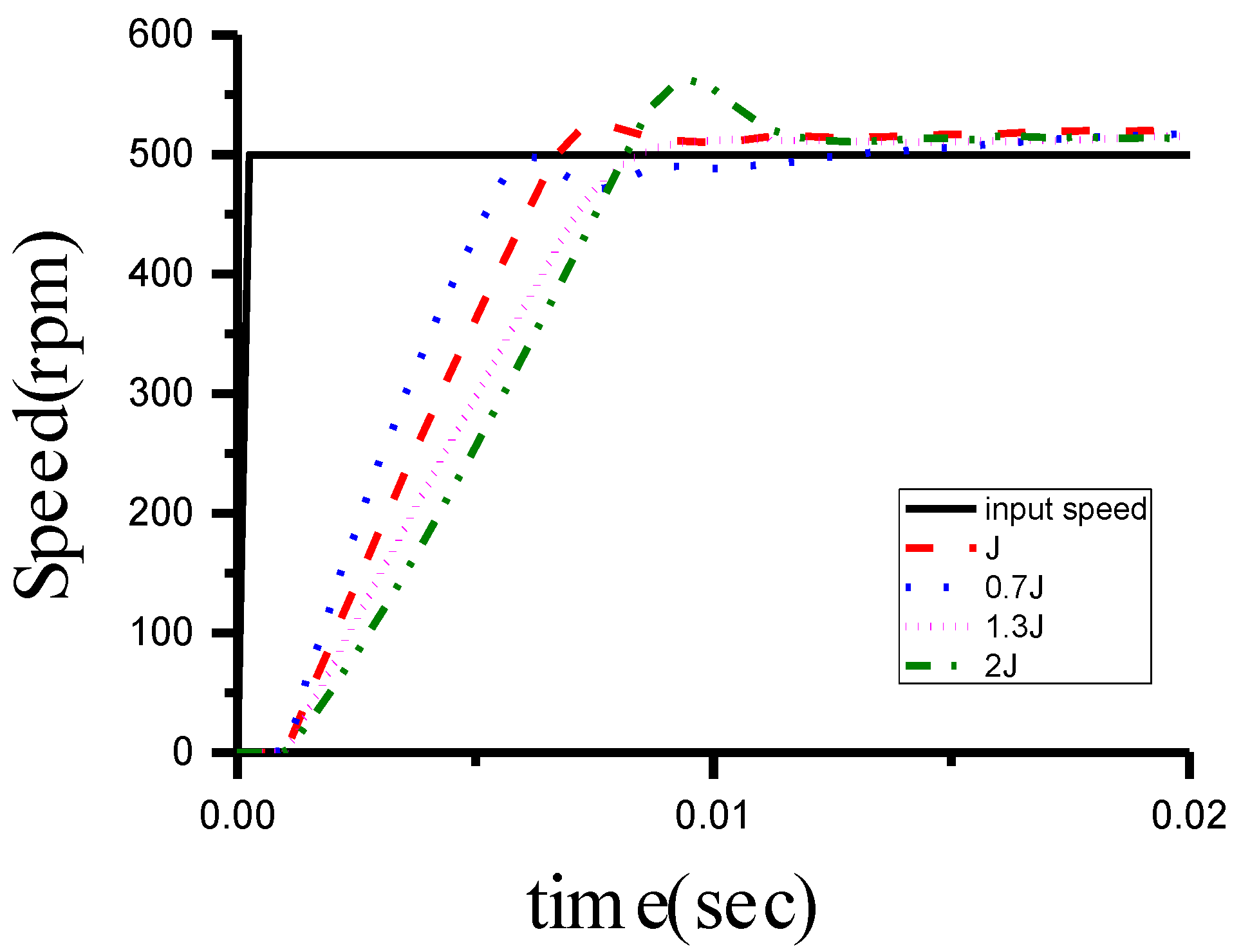
5.3. Inertia Simulation

Figure 11 shows the response of the system under different inertia errors. From this, it can be seen that when the load inertia has a certain input error, the above algorithm can still run stably with a good steady-state and dynamic performance, which proves that the system has a good robustness. It can be seen from Figure 6b that when the input inertia is smaller than the actual inertia, the observed load torque becomes much larger. In this way, the speed error due to the inertia is compensated for by the larger observed torque. Therefore, the CLTO can reduce the dependence of the system on the inertia. When the system reaches a steady-state, the observed load torque will converge to the true load torque, ensuring the steady-state balance. This is consistent with our theoretical analysis.

6. Experiment and Analysis

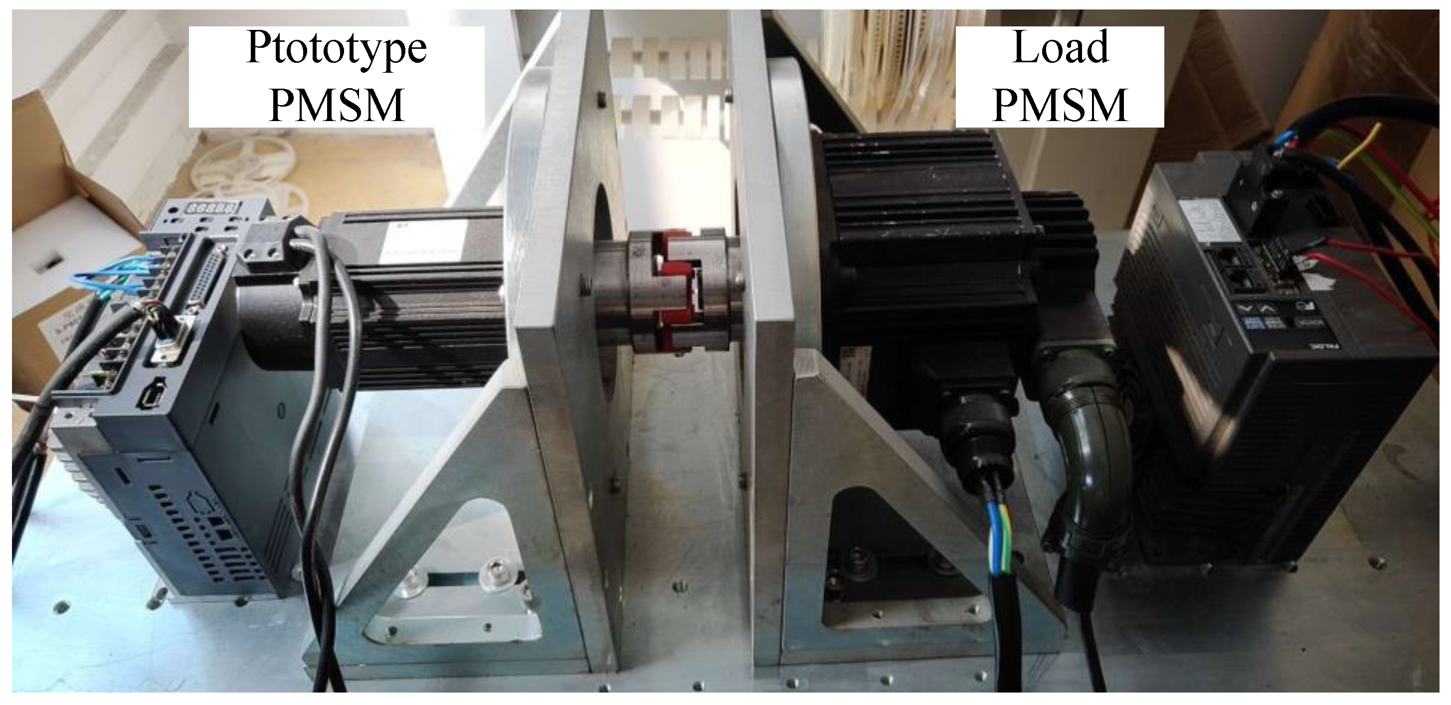
6.1. Experimental Platform Introduction

After simulations, the relevant experiments were carried out. The photographs of the experimental platform are shown in Figure 12. The parameters of the control board are shown in

Table 2. Parameters of the experimental platform.

Parameters	Values
Rated Power (W)	750
Rated Torque (Nm)	2.4
Rated Speed (Rpm)	3000
Rated Current (A)	4.5

. The control board is the servo-drive designed by ourselves, which is equipped with an NXP DSP KV3125612 microprocessor and an intelligent power module. With 220 V AC as the input, the output power of the servo-drive can reach up to 0.75 Kw, which belongs to a low power servo system. The load motor and load driver are Fuji RYC102C3-VVT2 and the rated output torque is 5 Nm. The current loop bandwidth of the experiment servo motor is 1 kHz, and the improved speed loop bandwidth of the servo system with a low-resolution encoder is 300 Hz, which is greatly improved compared with the M/T method.

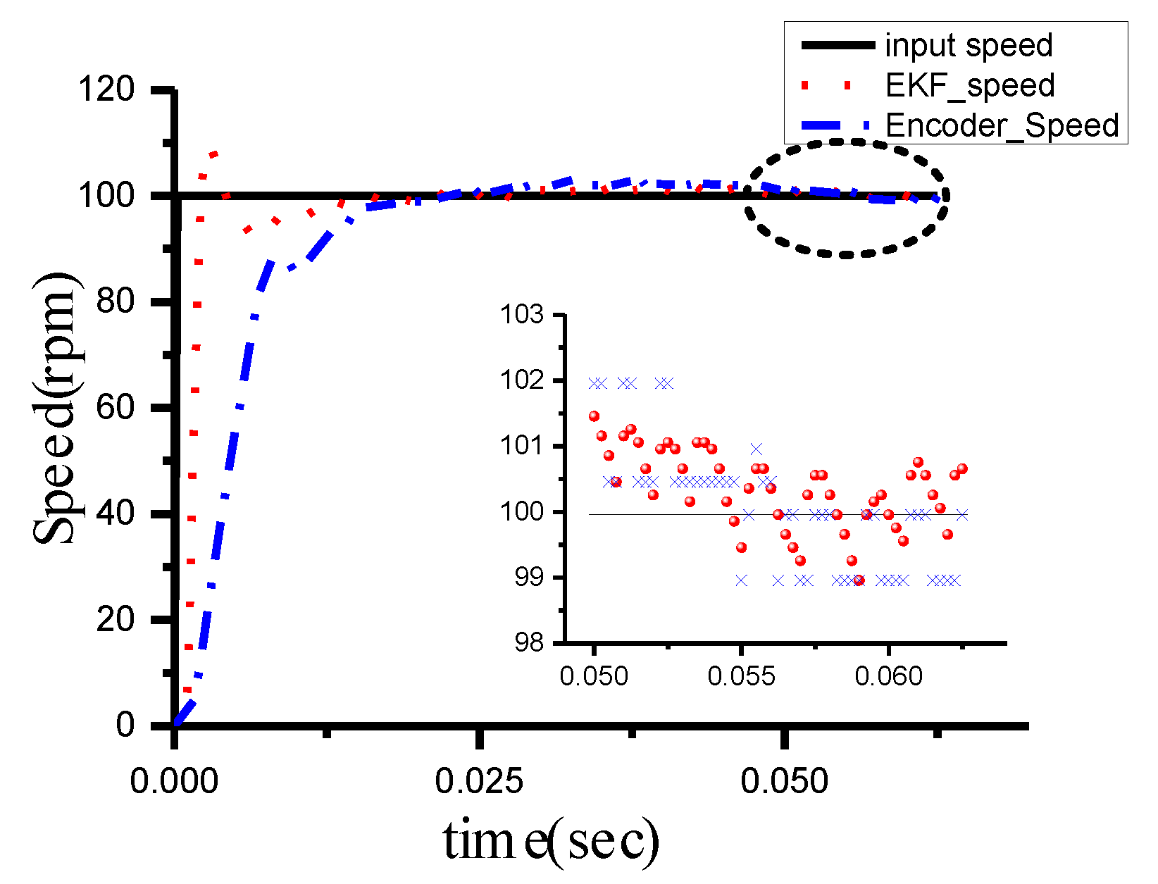
6.2. Step and Frequency Response Experiment

The above algorithm was tested by a step test through the experimental platform. As shown in Figure 13, the speed estimated by the reduced-order EKF has a faster response and is more stable than the speed calculated by the incremental photoelectric encoder. Figure 14 shows the speed response at very low-speed excitation (10 rpm) and very high-speed excitation (1000 rpm), respectively. It can be seen from the step response results under different speed excitations that the speed feedback estimated by EKF has a smaller feedback delay. The above results also show that the mentioned algorithm can run well at different speeds.

Figure 15 shows the speed response at 100 Hz and 200 Hz velocity excitation. It can be seen that the velocity estimated by EKF has a faster dynamic response and a smaller amplitude attenuation. Therefore, the cutoff frequency of the speed loop is extended and the dynamic performance of the speed loop is significantly improved. Through step experiments and frequency response experiments, it is verified that the control strategy with the reduced-order EKF for speed feedback has a faster dynamic response and less steady-state fluctuation. It also proves the effectivity and feasibility of the above algorithm.

6.3. Load Torque Experiment

Figure 16 shows the results of the speed feedback and observed load torque at 50 Hz excitation. Since the observed composite load torque includes a fixed load torque and a friction torque as a function of speed, the frequency of the observed composite torque should be consistent with the frequency of the speed feedback. The result shown in Figure 15b is consistent with the theoretical analysis. However, due to the delay of calculation, the phase of the observed composite load torque will have a certain hysteresis compared to the speed feedback. The actual load torque is 0.55 Nm, which is similar to the observed value (0.545 Nm).

6.4. Inertia Experiment

Figure 17 shows the results of the velocity step experiment under different inertia error. It can be seen that when the inertia is not matched, the speed estimated by the reduced-order EKF will have different time delays than the true speed. However, they can all work stably and the dynamic performance is not significantly degraded. Through the EKF equation, we can see that the inertia and torque are used to predict the change of speed and thus reduce the speed feedback delay. When the inertia does not match, it will lead to inaccurate prediction models, which will lead to speed prediction errors. However, the torque corrected by the PI controlled CLTO can be used to suppress the model error caused by the inertia error. This shows that the torque observer through PI convergence has a certain compensation effect on the inertia error, which improves the robustness of the algorithm. At the same time, the speed has different degrees of overshoot under different moments of inertia error. This is because, in practical applications, the choice of the speed loop parameter is related to inertia. When the input inertia is too large, the set PI parameter will be too large, resulting in a certain overshoot.

7. Conclusions

The improved speed loop control strategy performs well in terms of both a dynamic and steady-state performance. The experimental results of the step and frequency response show that it solves the problem of the large speed delay of the traditional M/T method in a low speed range. Using a CLTO to reduce the order of EKF can reduce the computational complexity of EKF and make it easy to use in different occasions. Through theoretical analysis and experiments, it is verified that the torque observer using the PI convergence method can effectively improve the robustness of the system. At the same time, the CLTO observed the load torque and the friction torque together, avoiding the problem that the coefficient of friction is not easy to measure in practical applications. The feasibility and effectivity of the above algorithm are verified by the simulations and experiments.

Due to limited capabilities, the above algorithm still has some limitations. For example, the dynamic response of the observed torque is not fast enough. More advanced parameter-insensitive torque observation methods are needed. More advanced control strategies need to be applied to the control of the speed loop. Further work will focus on more advanced control algorithms, more advanced torque observers, and inertia identification methods.

References

1. Ohmae, T.; Matsuda, T.; Kamiyama, K. A microprocessor-controlled high-accuracy wide-range speed regulator for motor drives. IEEE Trans. Ind. Electron. 1982, 29, 207–211. [Google Scholar] [CrossRef]
2. Robert, D.L.; Keith, W.V. High-resoolution velocity estimation for all-digital, ac servo drives. IEEE Trans. Ind. Appl. 1991, 27, 701–705. [Google Scholar]
3. Lee, S.H.; Lasky, T.A.; Velinsky, S.A. Improved velocity estimation for low-speed and transient regimes using low-resolution encoders. IEEE/ASME Trans. Mechatron. 2004, 9, 553–560. [Google Scholar] [CrossRef]
4. Saito, K.; Kamiyama, K.; Ohmae, T.; Matsuda, T. A microprocessor-controlled speed regulator with instantaneous speed estimation for motor drives. IEEE Trans. Ind. Electron. 1988, 35, 95–99. [Google Scholar] [CrossRef]
5. Ovaska, S.J. Improving the velocity sensing resolution of pulse encoders by FIR prediction. IEEE Trans. Instrum. Meas. 1991, 40, 657–658. [Google Scholar] [CrossRef]
6. Marc, B.; John, C.; Robert, T.N. Nonlinear speed observer for high-performance induction motor control. IEEE Trans. Ind. Electron. 1995, 42, 337–343. [Google Scholar]
7. Lee, S.H.; Song, J.B. Acceleration Estimator for low-velocity and low-acceleration regions based on encoder position data. IEEE/ASME Trans. Mechatron. 2001, 6, 337–343. [Google Scholar]
8. Su, Y.X.; Zheng, C.H.; Sun, D.; Duan, B.Y. A simple nonlinear velocity estimator for high-performance motion control. IEEE Trans. Ind. Electron. 2005, 52, 1161–1169. [Google Scholar] [CrossRef]
9. Mercorelli, P. A Motion-Sensorless Control for Intake Valves in Combustion Engines. IEEE Trans. Ind. Electron. 2017, 64, 3402–3412. [Google Scholar] [CrossRef]
10. Yang, S.M.; Ke, S.J. Performance evaluation of a velocity observer for accurate velocity estimation of servo motor drives. IEEE Trans. Ind. Appl. 2000, 36, 98–104. [Google Scholar] [CrossRef]
11. Kim, H.W.; Sul, S.K. A new motor speed estimator using Kalman filter in low-speed range. IEEE Trans. Ind. Electron. 1996, 43, 498–504. [Google Scholar]
12. Ali, W.H.; Gowda, M.; Cofie, P.; Fuller, J. Design of a speed controller using extended Kalman filter for PMSM. Trans. Int. Midwest Symp. Circuits Syst. 2014, 57, 1101–1104. [Google Scholar]
13. Bolognani, S.; Tubiana, L.; Zigliotto, M. Extended Kalman filter tuning in sensorless PMSM drives. IEEE Trans. Ind. Appl. 2003, 39, 1741–1747. [Google Scholar] [CrossRef]
14. Zheng, Z.D.; Fadel, M.; Li, Y.D. High performance PMSM sensorless control with load torque observation. Trans. China Electrotech. Soc. 2007, 22, 18–23. [Google Scholar]
15. Dhaouadi, R.; Mohan, N.; Norum, L. Design and implementation of an extended kalman filter for the state estimation of a permanent magnet synchronous motor. IEEE Trans. Power Electron. 1991, 6, 491–497. [Google Scholar] [CrossRef]
16. Bolognani, S.; Oboe, R.; Zigliotto, M. Sensorless full-digital PMSM drive with EKF estimation of speed and rotor position. IEEE Trans. Ind. Electron. 1999, 46, 184–191. [Google Scholar] [CrossRef]
17. Bolognani, S.; Zigliotto, M.; Zordan, M. Extended-range PMSM sensorless speed drive based on stochastic filtering. IEEE Trans. Power Electron. 2001, 16, 110–117. [Google Scholar] [CrossRef]
18. Park, J.B.; Wang, X. Sensorless Direct Torque Control of Surface-Mounted Permanent Magnet Synchronous Motors with Nonlinear Kalman Filtering. Energies 2018, 11, 969. [Google Scholar] [CrossRef]
19. Yang, M.; Liu, Z.; Long, J.; Qu, W.; Xu, D. An Algorithm for Online Inertia Identification and Load Torque Observation via Adaptive Kalman Observer-Recursive Least Squares. Energies 2018, 11, 778. [Google Scholar] [CrossRef]
20. Xu, B.; Mu, F.; Shi, G.; Ji, W.; Zhu, H. State Estimation of Permanent Magnet Synchronous Motor Using Improved Square Root UKF. Energies 2016, 9, 489. [Google Scholar] [CrossRef]
21. Chen, L.; Liu, S. A Kalman estimator for detecting repetitive disturbances. In Proceedings of the 2005, American Control Conference, Portland, OR, USA, 8–10 June 2005; Volume 3, pp. 1631–1636. [Google Scholar]
22. Masi, A.; Butcher, M.; Martino, M.; Picatos, R. An application of the extended Kalman filter for a sensorless stepper motor drive working with long cables. IEEE Trans. Ind. Electron. 2012, 59, 4217–4225. [Google Scholar] [CrossRef]
23. Alonge, F.; D’Ippolito, F.; Sferlazza, A. Sensorless control of induction-motor drive based on robust Kalman filter and adaptive speed estimation. IEEE Trans. Ind. Electron. 2014, 61, 1444–1453. [Google Scholar] [CrossRef]
24. Zarei, J.; Shokri, E. Convergence analysis of non-linear filtering based on cubature Kalman filter. IET Sci. Meas. Technol. 2015, 9, 294–305. [Google Scholar] [CrossRef]
25. Wang, X.; Yaz, E.E. Stochastically resilient extended Kalman filtering for discrete-time nonlinear systems with sensor failures. Int. J. Syst. Sci. 2014, 45, 1393–1401. [Google Scholar] [CrossRef]
Figure 1. The block diagram of the speed loop system.
Energies 11 02886 g001
Figure 2. The structure diagram of CLTO.
Energies 11 02886 g002
Figure 3. (a) The curve of EKF gain k0 varies with q0, and (b) the curve of EKF gain k1 varies with q0 (q1 = 12000, r = 0.1) (simulation).
Energies 11 02886 g003
Figure 4. (a) The curve of EKF gain k0 varies with q1, and (b) the curve of EKF gain k1 varies with q1 (q0 = 0.1, r = 0.1) (simulation).
Energies 11 02886 g004
Figure 5. (a) The speed response at different values of q0, and (b) partial amplification at a steady state (q1 = 12000, r = 0.1) (simulation).
Energies 11 02886 g005
Figure 6. (a) The speed response at different values of q1, and (b) partial amplification at a steady state (q0 = 0.1, r = 0.1) (simulation).
Energies 11 02886 g006
Figure 7. The speed response at different initial values of P0 (simulation).
Energies 11 02886 g007
Figure 8. Simulation result under 1000 rpm step excitation (simulation).
Energies 11 02886 g008
Figure 9. (a) Speed curve at load suddenly increases from 0.5 Nm to 1 Nm at 0.5 s, and (b) observed load torque (simulation).
Energies 11 02886 g009
Figure 10. (a) Speed curve at load suddenly decreases from 1 Nm to 0.5 Nm at 0.5 s, and (b) observed load torque (simulation).
Energies 11 02886 g010
Figure 11. (a) Speed step under different inertia error, and (b) simulation result of observed load torque (simulation).
Energies 11 02886 g011
Figure 12. Photographs of the experimental platform.
Energies 11 02886 g012
Figure 13. Step response and partial amplification at 100 rpm excitation (experiment).
Energies 11 02886 g013
Figure 14. Step response at (a) 10 rpm and (b) 1000 rpm speed excitation, respectively (experiment).
Energies 11 02886 g014
Figure 15. Loop response at (a) 100 Hz and (b) 200 Hz speed excitation, respectively (experiment).
Energies 11 02886 g015
Figure 16. (a) Loop response at 50 Hz speed excitation, and (b) observed load torque by CLTO (experiment).
Energies 11 02886 g016
Figure 17. Experimental results of velocity steps under different inertia error (experiment).
Energies 11 02886 g017