A New Input Selection Algorithm Using the Group Method of Data Handling and Bootstrap Method for Support Vector Regression Based Hourly Load Forecasting

Abstract

Electric load forecasting is indispensable for the effective planning and operation of power systems. Various decisions related to power systems depend on the future behavior of loads. In this paper, we propose a new input selection procedure, which combines the group method of data handling (GMDH) and bootstrap method for support vector regression based hourly load forecasting. To construct the GMDH network, a learning dataset is divided into training and test datasets by bootstrapping. After constructing GMDH networks several times, the inputs that appeared frequently in the input layers of the completed networks were selected as the significant inputs. Filter methods based on linear correlation and mutual information (MI) were employed as comparison methods, and the performance of hybrids of the filter methods and the proposed method were also confirmed. In total, five input selection methods were compared. To verify the performance of the proposed method, hourly load data from South Korea was used and the results of one-hour, one-day and one-week-ahead forecasts were investigated. The experimental results demonstrated that the proposed method has higher prediction accuracy compared with the filter methods. Among the five methods, a hybrid of an MI-based filter with the proposed method shows best prediction performance.

1. Introduction

Electric load forecasting (ELF) is essential for the effective and stable planning and operation of power systems [1]. Forecasting models are constructed based on historical load series and exogenous variables (e.g., weather, economic, and social factors), and the models are used to predict future loads for a specified period of time ahead. Various decisions related to power systems depend on the future behavior of loads, such as unit commitment, spinning reserve reduction, economic dispatch, automatic generation control, reliability analysis, maintenance scheduling, and energy commercialization [2,3]. ELF, especially, has major effects on deregulated electricity markets (e.g., demand response management [4,5,6]) and their participants because the prices on the markets are determined by the predicted future loads. Therefore, accurate and robust ELF can contribute greatly to decision making related to power systems. However, it is difficult to precisely forecast time-series loads because they exhibit a high degree of seasonality and nonlinear characteristics.

In recent decades, a wide range of methods has been proposed for ELF. In particular, artificial intelligence-based methods such as artificial neural networks (ANNs) [7,8,9,10] and support vector regression (SVR) [11,12,13,14,15] have been applied successfully to ELF due to their excellent learning capacity and nonlinear mapping ability without requiring any prior domain knowledge. However, ANNs based on the empirical risk minimization principle often suffer from over-fitting problems. Furthermore, when derivative-based optimization techniques are used for training ANNs, they are likely to be trapped in a local minimum. Compared to ANNs, over-fitting problems can be overcome in SVR because it is based on the structural risk minimization principle [16,17], i.e., the learning error and generalization capability are considered simultaneously.

The importance of ELF and its difficulty have motivated extensive studies, but the problem of input selection for ELF models remains an open question. In ELF, a major issue is selecting significant inputs (SIs) from many initial input candidates (IICs). Three main reasons necessitate input selection procedures [18,19]. First, properly selected inputs decrease the complexity of the model, and thus facilitate more efficient learning. Second, the forecasting performance can be improved by removing redundant inputs that are irrelevant to the outputs and dependent on other inputs. Finally, we can gain valuable insights into the fundamental features of loads and their prediction mechanism. In the following, we summarize several previous studies on input selection methods for load forecasting.

Ghofrani et al. [20] proposed a new input selection framework by combining correlation analysis and the l²-norm for short-term load forecasting (STLF). Koprinska et al. [21] used mutual information (MI), RReliefF, and a correlation-based method for feature selection of the load forecasting model. Sheikhan and Mohammadi [22] developed a feature selection method by combining a genetic algorithm with ant colony optimization for STLF. Tikka and Hollmén [23] proposed sequential backward input selection for ELF, which is based on a linear model and a cross-validation resampling procedure. Sorjamaa et al. [24] combined a direct prediction strategy with three input selection criteria, i.e., k-nearest neighbors approximation method, MI, and nonparametric noise estimation, for ELF. Da Silva et al. [25] used filter methods based on phase-space embedding and MI and Bayesian wrapper methods for ANN-based ELF. Hu et al. [19] proposed a hybrid filter-wrapper approach with a partial MI and firefly algorithm for STLF feature selection.

In general, the methods mentioned above can be categorized as filter (model-free) or wrapper (model-based) methods [26,27,28,29]. In filter methods, after statistical analyses between the potential inputs and output, the inputs with strong relationships to the output are selected as SIs. In wrapper methods, the accuracy of learning machines is used as a selection criterion and the best input combinations are explored by sequential search procedures, such as backward elimination, forward selection, stepwise selection, and metaheuristics. Filter methods can select SIs without learning machines, but these methods do not consider the prediction accuracy, and thus they often perform worse than wrapper methods. Linear correlation (LC) analysis, frequently used in filter methods, with nonlinear predictors can degrade the forecasting performance because they cannot identify nonlinear relationships between inputs and output. In wrapper approaches, the best input combinations are determined by the sequential search procedures, so the computational complexity grows exponentially with the number of IICs. Furthermore, depending on the structure and parameter identification methods used for wrappers, biased input selection results may be obtained.

In summary, instead of only considering the one-to-one statistical correlations, input selection methods for data-driven load forecasting should be able to tackle both the many-to-one nonlinear relationships between dependent and independent variables and the accuracy of the forecasting machines.

In this paper, we propose a new input selection procedure based on the group method of data handling (GMDH) and the bootstrap method for ELF. Although there are several previous studies where GMDH is employed for ELF [30,31], this paper is the first attempt to use GMDH only for input selection. Generally, GMDH networks have been widely used for modeling the nonlinear relationships between variables. Compared with the previous approaches, this paper focuses on the fact that, based only on a given dataset, the GMDH algorithm can not only determine the network structures but also select the inputs with significant explanatory powers for predicting the outputs. In the GMDH algorithm, the GMDH networks where polynomial neurons are hierarchically connected with each other are automatically constructed using learning datasets collected from target systems. Among a number of IICs, the remaining elements in the input layer of the finally constructed GMDH network are considered as relevant inputs. The learning dataset should be divided into training and test datasets to construct the GMDH network. In this study, bootstrap method is applied for the data division. The learning dataset is divided randomly by bootstrap sampling, so the relevant inputs are different each time. Therefore, in the proposed method, after constructing GMDH networks several times using bootstrapping, the inputs that appear frequently in the input layers of the completed networks are finally selected as the SIs.

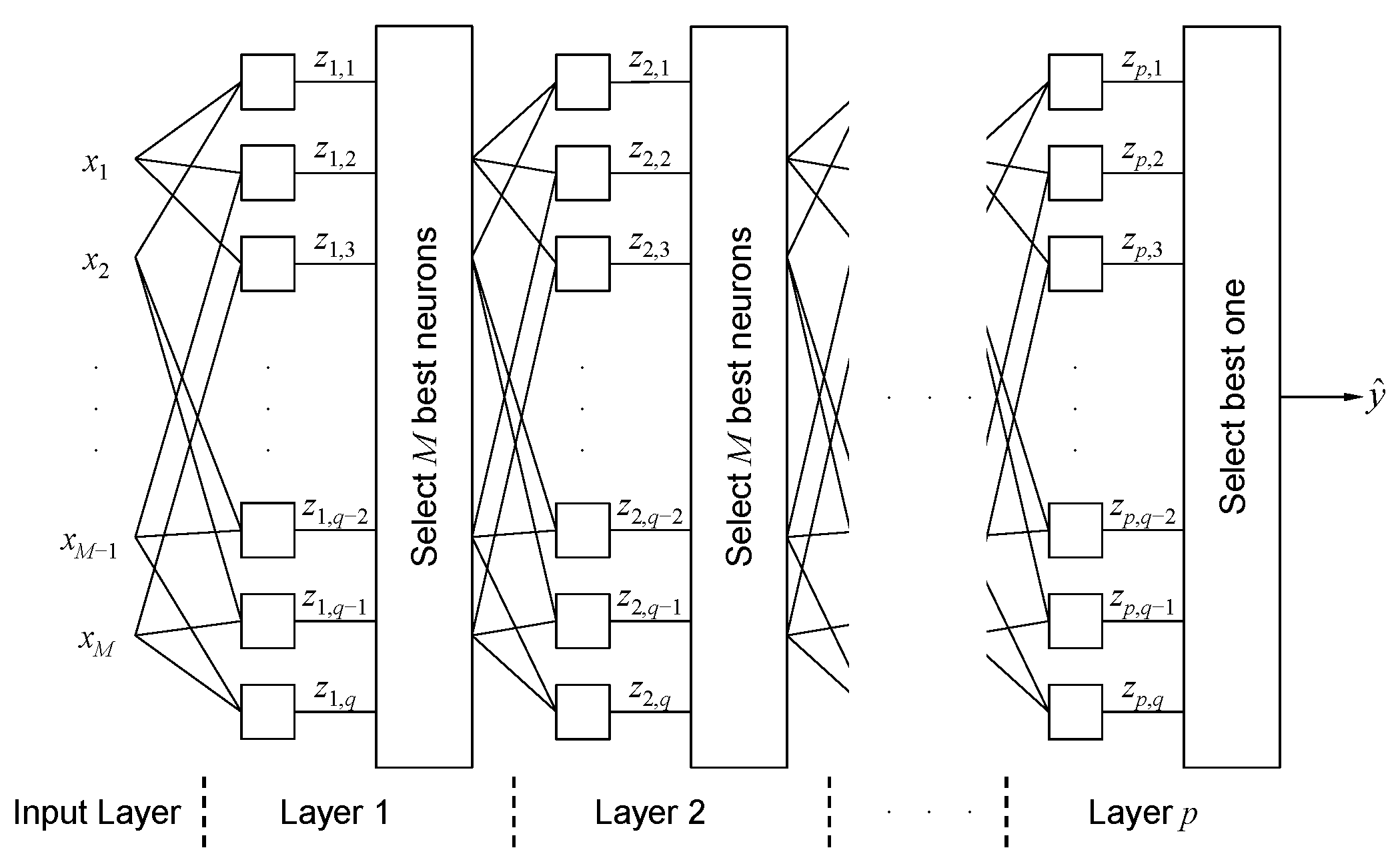
The main advantages of the proposed input selection method combining the GMDH and bootstrap method can be briefly summarized as follows. First, based on the GMDH network structures in which the polynomial neurons are hierarchically connected with each other (see Figure 1), the method can select significant inputs by taking many-to-one nonlinear relationships between explanatory and target variables into consideration. Second, since prediction accuracy is used as the input selection criterion (see Section 2.2), it is expected that the method achieves improved forecasting performance compared to filter methods based only on the statistical analyses.

To verify the performance of the proposed method, we use hourly load data from South Korea with seasonality, weekly and daily periodicity. LC- and MI-based filter methods are employed as comparison methods. In addition, hybrid approaches that combine the filter methods with the proposed method are also examined. In total, five input selection methods are investigated. Prediction models are constructed via ν-SVR, and we compare the one-hour, one-day, and one-week-ahead forecasting performance of the five input selection methods.

The remainder of this paper is organized as follows. Section 2 explains the procedure for GMDH network building. In Section 3, the new input selection method based on GMDH and bootstrap sampling, LC- and MI-based filter methods, and hybrid approaches are described. Section 4 briefly summarizes ν-SVR. In Section 5, we present the experimental results, and discuss the results in detail in Section 6. Finally, we give our conclusions in Section 7.

2. Group Method of Data Handling

Ivakhnenko first proposed the GMDH algorithm in 1968, which is a self-organizing modeling technique [32,33,34]. In the GMDH method, as shown in Figure 1, complex and nonlinear modeling is performed by the GMDH network where polynomial neurons are hierarchically connected in a forward direction.

A quadratic two-variable polynomial is commonly used as a transfer function for each neuron and their coefficients can be estimated by the least-squares method. When the number of entering inputs and/or the order of the polynomials become larger, the number of parameters to be estimated rapidly increases. To build a GMDH network, only the learning dataset collected from target systems is needed, and relevant inputs as well as the network structure can be determined automatically.

Let $D={\{x_k;y_k\}}_{k=1}^n$ be a learning dataset for GMDH network building, where x = [x₁, x₂, …, x_M]^T is an input vector composed of IICs and M is the number of the IICs. In layer 1, (q = M(M − 1)/2) neurons that consider all combinations of the initial inputs are generated and only the outputs of M neurons that satisfy a selection criterion are used as inputs for the next layer. In the same manner, q neurons are generated from layer 2 based on the M neurons selected in the previous layer. This layer extension process continues in a forward direction until a stopping criterion is satisfied. After stopping the extension process, the output layer and neuron are fixed and all of the elements connected with the output neuron are found sequentially by backward search.

2.1. Parameter Estimation for Polynomial Neurons

In the GMDH network, the output, z, of an arbitrary neuron is calculated as

$$z=f(x_u,x_l;\mathsf{\theta })={\theta }_0+{\theta }_1{x}_u+{\theta }_2{x}_l+{\theta }_3{(x_u)}^2+{\theta }_4{(x_l)}^2+{\theta }_5{x}_u{x}_l,$$

(1)

where x_u and x_l are two inputs of the neuron and θ = [θ₀, …, θ₅]^T is composed of its polynomial coefficients. The same learning dataset D is employed repeatedly to estimate parameters for each neuron. After substituting D into (1), the n linear equations are formulated in concise matrix form, i.e., Xθ = z. Using the least-squares method, the parameter vector θ can be optimized as

$$\widehat{\mathsf{\theta }}={(X^{T}X)}^{-1}{X}^{T}z.$$

(2)

In (2), if the determinant of X^TX is close to zero, then the estimator $\widehat{\mathsf{\theta }}$ is rather susceptible to round off errors and its performance deteriorates. In this study, the polynomial coefficients are estimated using singular value decomposition, as follows [35,36]:

$${\widehat{\mathsf{\theta }}}^{+}=X^{+}z=V{S}^{+}{U}^{T}z,$$

(3)

where X⁺ is the pseudo-inverse of X, the columns of matrices V and U correspond to the eigenvectors of X^TX and XX^T, respectively, and the main diagonal components of S⁺ are composed of the reciprocals of r singular values.

2.2. Construction of the GMDH Network

To build the GMDH network, layer extension is performed in the forward direction until the stopping criterion is satisfied. Next, the output layer and neuron are fixed and a search for all of the elements connected to the output neuron is conducted by backward tracing, i.e., from the output to input layer. After finishing the search in the backward direction, we can obtain not only the GMDH network structure, but also relevant inputs in the input layer.

In the proposed method, checking error criterion (CEC) [37] is employed: (1) to select the neurons whose outputs will be used as inputs for the next layer; and (2) to determine whether the layer extension process should be stopped. The number of layers in the GMDH networks is closely related to the model’s complexity. The deeper the networks, the more complex their structures; in this case, many unnecessary inputs can be selected together with significant inputs. On the other hand, if the networks are too shallow, input variables with great explanatory powers can be missed. To calculate the CEC, the learning dataset D is separated into dataset A, $D_A={\{x_k^A;y_k^A\}}_{k=1}^{n_A}$, and dataset B, $D_B={\{x_k^B;y_k^B\}}_{k=1}^{n_B}$, using the bootstrap method [38]. In the bootstrap method, after applying n sampling with replacement to D, we obtain n data pairs. Each data pair in D has the same probability of being selected during the sampling process. Among the n sampled data pairs, only unique pairs comprise D_A for training and D_B consists of the remaining data pairs, i.e., D_B = D\D_A for testing. The ratio of D_A relative to D_B is approximately 6:4.

Using D_A, the parameter vector of a neuron is estimated by (3) and the outputs are calculated based on D_B, ${\widehat{y}}_k^B=f\left({(x_u)}_k^B,{(x_l)}_k^B;{({\widehat{\mathsf{\theta }}}^{+})}^A\right)$, k = 1, …, n_B. The CEC of the neuron is computed by

$$CEC=\sqrt{\frac{1}{n_B}{\displaystyle \sum _{k=1}^{n_B}{(y_k^B-{\widehat{y}}_k^B)}^2}}.$$

(4)

After calculating the CEC for q neurons in the ith layer, i.e., CEC(i, j), j = 1, …, q, they are arranged in ascending order and only the M neurons with the smallest CEC values are selected. If an early stopping condition, CEC(i − 1) ≤ CEC(i), i ≥ 2, (where CEC(i) = min_j{CEC(i, j)}, j = 1, …, q), is satisfied or the current layer is equal to the predefined maximum layer, then the layer extension is halted. Then, the output layer p^* and output neuron q^* are selected as follows:

$$p^{*}=\underset{i}{\arg \min }\{CEC(i)\},$$

(5)

$$q^{*}=\underset{j}{\arg \min }\{CEC(p^{*},j)\},j=1,\cdots ,q.$$

(6)

After selecting the output neuron, all of the elements connected with the neuron are found by a sequential search in the backward direction. In each layer, neurons without any connections to the output neuron are removed and the remaining neurons and their connections are preserved. The GMDH network is finally constructed after finishing the backward search from the output to input layer. Algorithm 1 describes the procedure for constructing the GMDH network.

Algorithm 1. Constructing the GMDH network.

Input: learning dataset D Divide D into DA and DB using bootstrap method Imax ← maximum layer BN ← {x1, …, xM} //where BN denotes the set of ‘best neurons’. for i from 1 to Imax  Create (q = M(M − 1)/2) neurons in ith layer based on BN  for j from 1 to q   Estimate ${({\widehat{\mathsf{\theta }}}^{+})}^A$ of jth neuron using DA   Calculate CEC(i, j) for jth neuron using DB  end  CEC(i) = minj{CEC(i, j)}, j = 1, …, q  if i ≥ 2 then   if CEC(i − 1) ≤ CEC(i) then    break this loop   end  end  BN ← M neurons in ith layers with smallest CEC(i, j), j = 1, …, q end p* ← argmini{CEC(i)} q* ← argminj{CEC(p*, j)} Remove all neurons in p*th layer except for q*th neuron p ← p* repeat  p ← p − 1  Find the neurons in pth layer connected with neurons in (p + 1)th layer  Remove all neurons and their connections in pth layer except for the founded neurons until p == 0   return GMDH network structure and a set of relevant inputs, $X=\{x_1,\cdots ,x_m\}(\subset \{x_1,\cdots ,x_M\})$

From the final constructed GMDH network, we can confirm the inputs in the input layer connected with the output neuron and they are regarded as relevant inputs.

3. Input Selection Method

In this study, to select the inputs for ELF models, we employed: (1) LC- and MI-based filter methods, (2) GMDH-based and bootstrapping-based input selection (i.e., the proposed method), and (3) hybrid methods that combine filter methods with GMDH-based input selection.

3.1. Filter Methods Based on LC and MI

In this subsection, we explain the LC- and MI-based filter methods (i.e., comparison methods). In the filter methods, we calculated the ranking function (RF) values, RF(x_j, y), j = 1, …, M, between all of the potential inputs and output. The inputs with RF values that are greater than or equal to the threshold value RF_th were selected as SIs. More details regarding the LC and MI used as RF are available elsewhere [28,29,39,40]. Among M IICs {x₁, …, x_M}, m SIs {x_1st, x_2nd, …, x_mth} are determined as

$$\{x_{1\mathrm{st}},x_{2\mathrm{nd}},\cdots ,x_{m\mathrm{th}}\}=\left\{x_j\right|RF(x_j,y)\ge R{F}_{\mathrm{th}},j=1,\cdots ,M\},$$

(7)

where the condition, $RF(x_{1\mathrm{st}},y)>\cdots >RF(x_{m\mathrm{th}},y)$, is satisfied.

3.2. The Proposed Method: GMDH-Based and Bootstrapping-Based Input Selection

As explained in Section 2, the components of the input layer in the finished GMDH network are considered as relevant inputs. Since D is divided randomly into D_A and D_B by bootstrap sampling, the input selection results will vary in each experiment. Moreover, the relevant inputs obtained by constructing only a single network may yield biased results. Thus, in the proposed method, input selection was performed according to the following procedures. Firstly, the GMDH networks were constructed r times in the same experimental conditions. The set of relevant inputs from the ith experiment is denoted as X_i, i = 1, …, r and their union is $X={\displaystyle {\cup }_{i=1}^r{X}_i}$. Then, in the union X, the total number, N_j, of each IIC, x_j, j = 1, …, M, is counted. Finally, the inputs for which N_j is greater than or equal to a predefined threshold, N_th, were selected as SIs. Algorithm 2 describes the GMDH- and bootstrap-based input selection procedures.

Algorithm 2. GMDH-based and bootstrap-based input selection.

Input: learning dataset D r ← the number of network constructions Nth ← threshold value X ← {} for i from 1 to r  Divide D into DA and DB using bootstrap method  Select relevant input set Xi using Algorithm 1  X ← $X\cup X_i$ end Count the number of xj, j = 1, …, M, Nj, in X {x1st, x2nd, …, xmth} = {xj|Nj ≥ Nth, j = 1, …, M}   return {x1st, x2nd, …, xmth}

3.3. Hybrid Input Selection Method

The hybrid input selection procedures that combine filter methods and the proposed method were carried out according to two phases. First, many redundant inputs were eliminated by applying LC- or MI-based filter methods to IICs. After then, the proposed input selection procedure described in Algorithm 2 was applied to the remaining inputs.

4. ν-Support Vector Regression

In this section, we briefly summarize ν-SVR [41] as proposed by Schölkopf et al. Let ${\{(x_i;y_i)\}}_{i=1}^l$ denote a collected learning dataset, where $x_i\in {\Re }^n$ is an n-dimensional input vector and $y_i\in {\Re }^1$ is the target output. The basic idea of SVR is to find a linear regression function after transforming the original space into a high-dimensional feature space, which is defined as

$$f(x)=w^T\varphi (x)+b,$$

(8)

where ϕ(∙) is a nonlinear mapping function from the input to feature space, and w and b are parameters of f that should be estimated from the learning dataset. The constrained optimization problem of ν-SVR is defined by introducing two positive slack variables ${\xi }_i$ and ${\xi }_i^{*}$, as follows [42]:

$$\begin{array}{l}\underset{w,b,\xi ,{\xi }^{*},\epsilon }{\min }\frac{1}{2}{\Vert w\Vert }^2+C\left(\nu \epsilon +\frac{1}{l}{\displaystyle \sum _{i=1}^l\left({\xi }_i+{\xi }_i^{*}\right)}\right)\\ \mathrm{subject} \mathrm{to} \{\begin{array}{l}\left(w^T\varphi (x_i)+b\right)-y_i\le \epsilon +{\xi }_i,\\ y_i-\left(w^T\varphi (x_i)+b\right)\le \epsilon +{\xi }_i^{*},\\ {\xi }_i,{\xi }_i^{*}\ge 0,i=1,\cdots ,l,\epsilon \ge 0.\end{array}\end{array}$$

(9)

where $\frac{1}{2}{\Vert w\Vert }^2$ is a regularization term, the parameter $\nu \in (0,1]$ controls the number of support vectors and training errors, and C is a regularization constant that determines the tradeoff between the model’s complexity and its accuracy. The training errors of regression function f are penalized by ξ_i and ξ_i^*, if they are larger than ε. The size of ε is traded off against the model’s complexity and slack variables via a constant ν [41]. As described in (9), SVR avoids under-fitting and over-fitting by minimizing both the regularization term and training errors.

By introducing Lagrange multipliers α_i and α_i^*, and applying Karush-Kuhn-Tucker conditions [43], the constrained optimization problem given by (9) is reformulated as follows:

$$\begin{array}{l}\underset{\mathsf{\alpha },{\mathsf{\alpha }}^{*}}{\min }\frac{1}{2}{\left(\mathsf{\alpha }-{\mathsf{\alpha }}^{*}\right)}^{T}Q\left(\mathsf{\alpha }-{\mathsf{\alpha }}^{*}\right)+y^T\left(\mathsf{\alpha }-{\mathsf{\alpha }}^{*}\right)\\ \mathrm{subject} \mathrm{to} \{\begin{array}{l}{\displaystyle \sum _{i=1}^l\left(\alpha -{\alpha }^{*}\right)}=0,{\displaystyle \sum _{i=1}^l\left(\alpha -{\alpha }^{*}\right)}=0\le C\nu ,\\ 0\le {\alpha }_i,{\alpha }_i^{*}\le C/l,i=1,\cdots ,l.\end{array}\end{array}$$

(10)

where Q is a kernel matrix and its entry in the ith row and jth column is Q_i,j = K(x_i, x_j) ≡ ϕ(x_i)^Tϕ(x_j). The kernel function K(x_i, x_j) defined in the input space is the same as the inner product of x_i and x_j in the feature space. The nonlinear mapping and inner products can be calculated in the original input space using the kernel function. In this paper, among the widely used kernel functions, such as polynomial, radial basis function (RBF), and sigmoidal kernels, we employed the RBF kernel function defined as

$$K(x_i,x)=\exp \left(-\gamma {\Vert x_i-x\Vert }^2\right),$$

(11)

where γ controls the width of the RBF function. By solving (10), we can obtain the approximated regression function as follows:

$$\widehat{f}\left(x\right)={\displaystyle \sum _{i=1}^l\left({\alpha }_i^{*}-{\alpha }_i\right)K\left(x_i,x\right)}+b.$$

(12)

The prediction accuracy of ν-SVR depends on the selection of appropriate design parameters, i.e., ν, C, and γ. Trial and error, cross-validation, grid search, and global optimization have been applied widely for determining the parameter values [2]. The aim of this paper is to examine the performance of the proposed input selection methods, so the procedures for selecting the design parameters will not be described in detail. In this study, the method presented in [3] is used to determine the design parameters.

5. Experimental Results

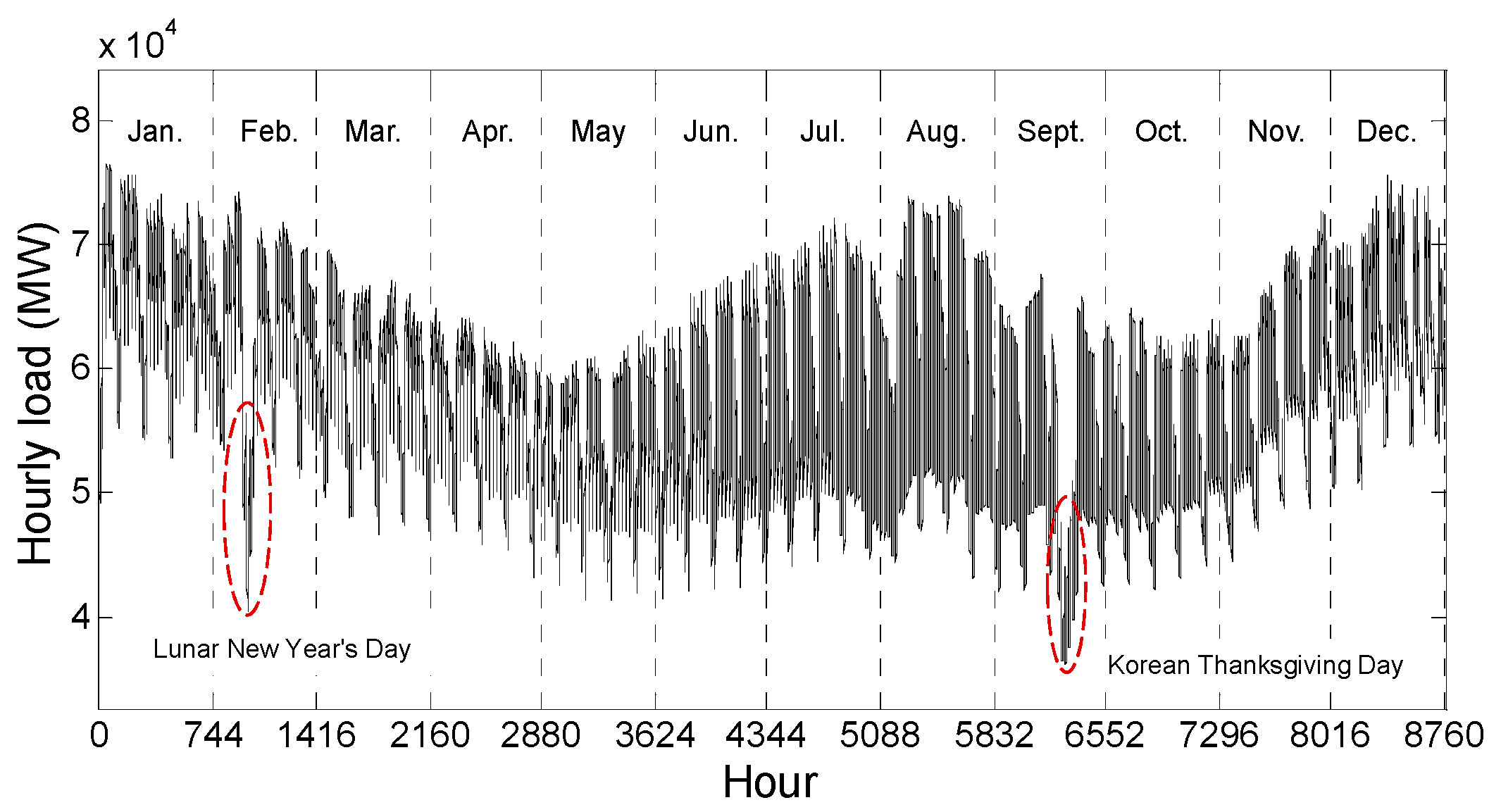
To verify the performance of the proposed method, hourly load data from South Korea between 1 January 2012 and 31 December 2014 was used. Figure 2 shows the hourly load curves for South Korea during one year (i.e., 2013) and Figure 3 shows an example of the weekly profile for the curves during three weeks from 7 January 2013 until 27 January 2013.

As shown in Figure 2 and Figure 3, the target loads exhibit clear seasonality with weekly and daily periodicities. The load demand is usually higher in the summer and winter seasons compared with the spring and autumn seasons. The demand for electricity is higher on weekdays (from Monday to Friday) compared with weekends and the load demand is slightly higher on Saturday than Sunday. The minimum load on Monday is lower than that on other working days. In addition, the load demand on special days (e.g., national holidays and election days) exhibit remarkably unusual behavior. In this paper, we are not concerned with hourly load forecasting on special days, i.e., we focus only on hourly load forecasting for ordinary days.

To validate the seasonal forecasting performance, we select three months as validation months, i.e., April, July and November in 2014, where the objective is to predict their hourly load demands one hour, one day, and one week ahead. For the one-day and one-week-ahead forecasts that correspond to multi-step-ahead predictions, we employed the recursive strategy [44] explained in Appendix A.

5.1. Data Preparation

To prepare the learning dataset, we considered historical time-series load data {φ_t, t = 1, …, N}. For example, to predict the hourly load demand from 1 to 30 April in 2014, the load data from 1 January 2012 to 31 March 2014 is employed to prepare the learning data. After organizing the learning data matrix described in (13) using N historical data, the max-min normalization process is applied to each column as presented in (14).

$$\mathsf{\Phi }=\left[\begin{array}{ccccc}{\phi }_d& {\phi }_{d-1}& \cdots & {\phi }_1& {\phi }_{d+1}\\ {\phi }_{d+1}& {\phi }_d& \cdots & {\phi }_2& {\phi }_{d+2}\\ ⋮& ⋮& \ddots & ⋮& ⋮\\ {\phi }_{N-1}& {\phi }_{N-2}& \cdots & {\phi }_{N-d}& {\phi }_N\end{array}\right].$$

(13)

$${\mathsf{\Phi }}_{i,j}^{\prime }=\frac{{\mathsf{\Phi }}_{i,j}-\underset{i}{\min }\left\{{\mathsf{\Phi }}_{i,j}\right\}}{\underset{i}{\max }\left\{{\mathsf{\Phi }}_{i,j}\right\}-\underset{i}{\min }\left\{{\mathsf{\Phi }}_{i,j}\right\}}.$$

(14)

where Φ_i,j is the original component in the ith row and jth column of Φ and Φ′_i,j is its normalized value. The learning data matrix is an (N − d) × (d + 1) matrix, where d is the window size, i.e., the number of IICs. In this paper, to capture the daily and weekly periodicities of the target load, we chose a one-week window size, i.e., d = 168. The last column in Φ is composed of the desired outputs and the remaining columns consist of 168 IICs. Each row vector in Φ corresponds to an input-output learning data pair.

To take account of the seasonality, we reformulated a new matrix Φ_new composed of the row vectors of Φ, where the last column’s components (i.e., desired outputs) only correspond to the load values of a validation month and the previous month. For example, to forecast the hourly load during April in 2014, Φ_new is made up of row vectors where the desired outputs correspond to the hourly load during March and April in 2012 and 2013 and March in 2014.

Finally, the row vectors that contain hourly load values on special days are removed from Φ_new. In other words, if only one component of the row vectors corresponds to the hourly load for special days, the row vectors are discarded. This is necessary because the hourly load curves for special days have different shapes from those for normal days. If the prediction models for normal days are trained by learning data with load values on special days, biased forecasting results could be obtained.

The input selection methods explained in Section 3 were applied to the learning dataset prepared according to the procedures described above.

5.2. Input Selection Results

In this subsection, we present the results of applying the input selection methods to the prepared learning dataset. As explained in Section 3, we employed five input selection methods, which are abbreviated as follows.

(1)

‘LC’: LC-based filter method.

(2)

‘MI’: MI-based filter method.

(3)

‘GMDH’: the proposed method described in Algorithm 2.

(4)

‘LC + GMDH’: hybrid input selection method combining ‘LC’ and ‘GMDH’.

(5)

‘MI + GMDH’: hybrid input selection method combining ‘MI’ and ‘GMDH’.

(Note: The acronyms, LC and MI, denote the RFs, but the abbreviations, ‘LC’ and ‘MI’, refer to the LC- and MI-based filter methods.)

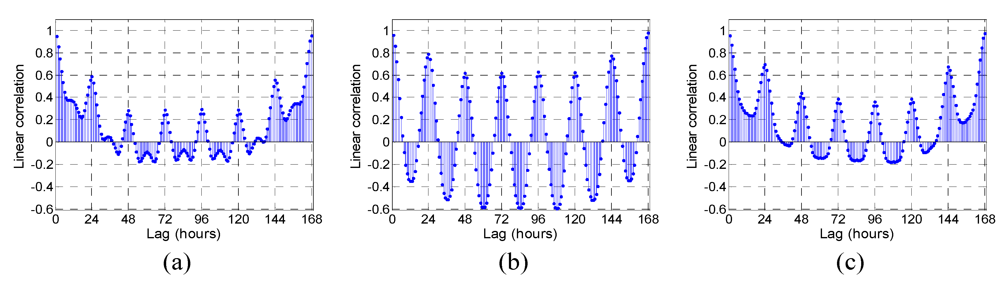
Figure 4 and Figure 5 show the LC and MI values calculated using the prepared learning dataset for predicting the loads in April, July and November in 2014.

In Figure 5, the MI values are normalized in a range of [0, 1]. Figure 4 and Figure 5 demonstrate that the shapes of LC and MI differ from the validation months because the target loads exhibit distinct seasonal behaviors. Daily and weekly periodicities can also be observed in these figures. In the filter methods based on LC and MI, after rearranging the calculated RF values in descending order, m inputs with RF values greater than or equal to the predefined RF_th are finally selected as SIs. 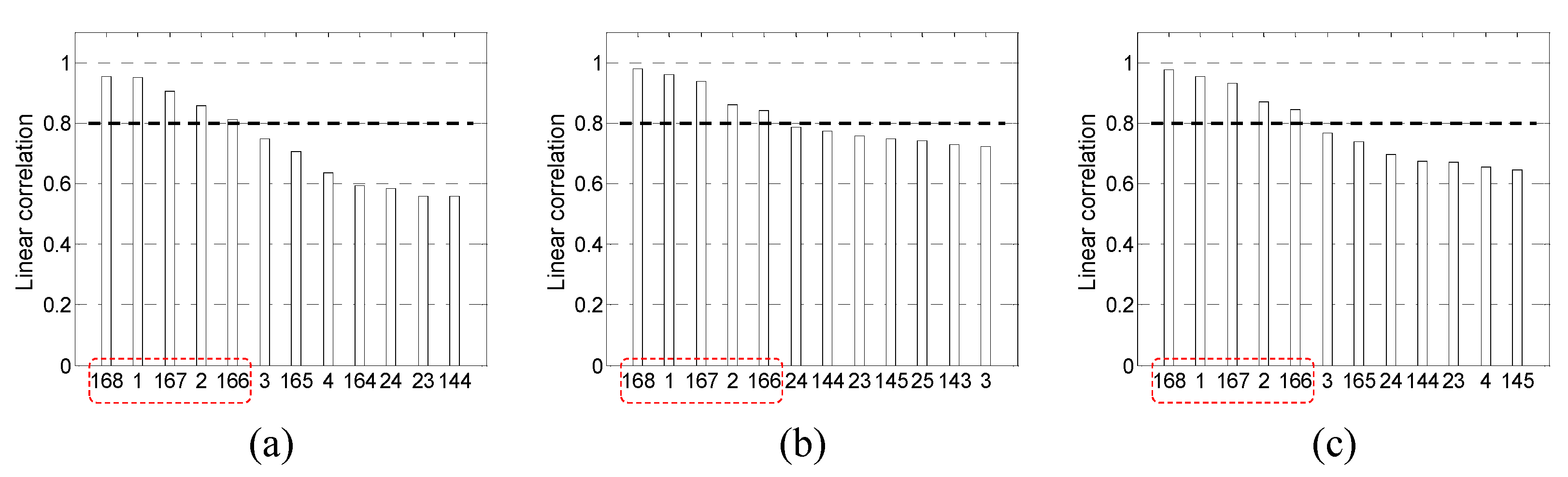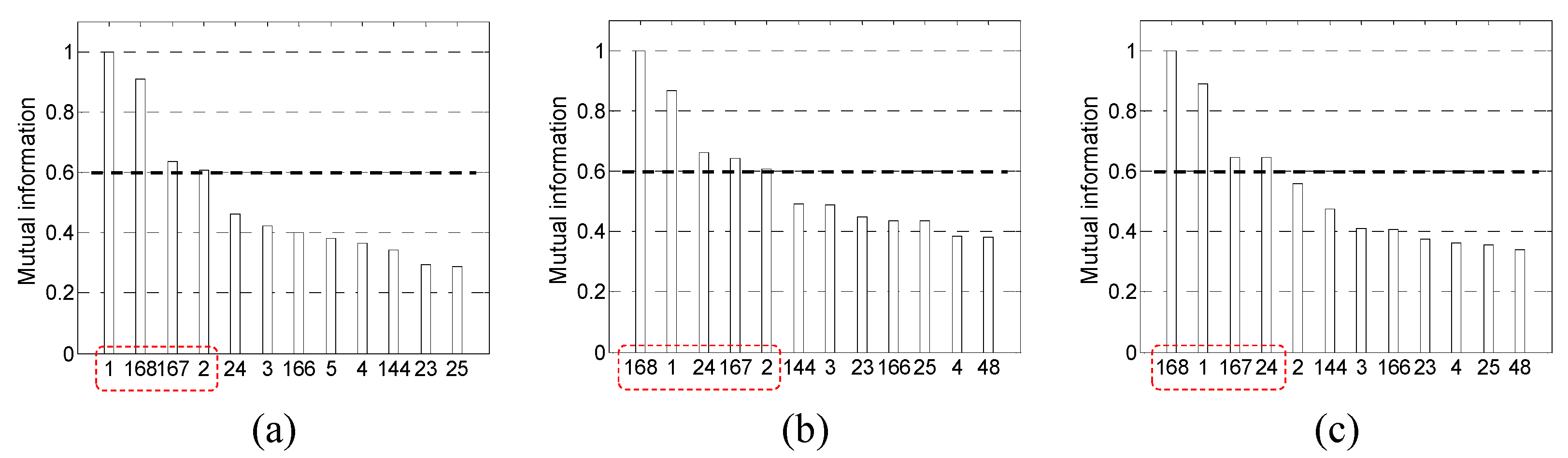Figure 6 and Figure 7 show the input selection results using ‘LC’ and ‘MI’.

As shown in Figure 6 and Figure 7, the threshold values for LC and MI are set as 0.8 and 0.6, respectively, and they are indicated by dashed thick solid black lines. The selected inputs are indicated by dashed red lines in the figures.

As explained in Section 3.2, in the ‘GMDH’, GMDH networks were constructed independently r times on the same conditions. In this paper, r is set to 30. In

Table 1. Example illustrating the application of Algorithm 1 30 times independently to the prepared learning dataset for predicting the loads in April 2014. The IICs and output are {φ_t−d+1, d = 1, 2, …, 168} and φ_t+1, respectively.

Experiment, i	Set of Relevant Inputs, Xi
1	X1 = {φt−d+1|d = 1, 2, 5, 7, 8, 22, 23, 135, 167, 168}
2	X2 = {φt−d+1|d = 1, 2, 6, 7, 24, 25, 167, 168}
3	X3 = {φt−d+1|d = 1, 2, 4, 7, 21, 24, 48, 49, 167, 168}
⁞	⁞
30	X30 = {φt−d+1|d = 1, 2, 6, 7, 21, 23, 24, 96, 167, 168}

, and the maximum layer, I_max, is set to 5 based on several trial-and-errors. Note that I_max corresponds to the maximum acceptable depth of the GMDH networks. Through several prior experiments, we confirmed that the forecasting performance may be degraded when I_max is too large (e.g., I_max ≥ 7) or too small (e.g., I_max ≤ 3). If I_max is set to be excessively large values, and consequently, too many inputs are selected, then it is difficult to intuitively understand the predictive principles of target data. 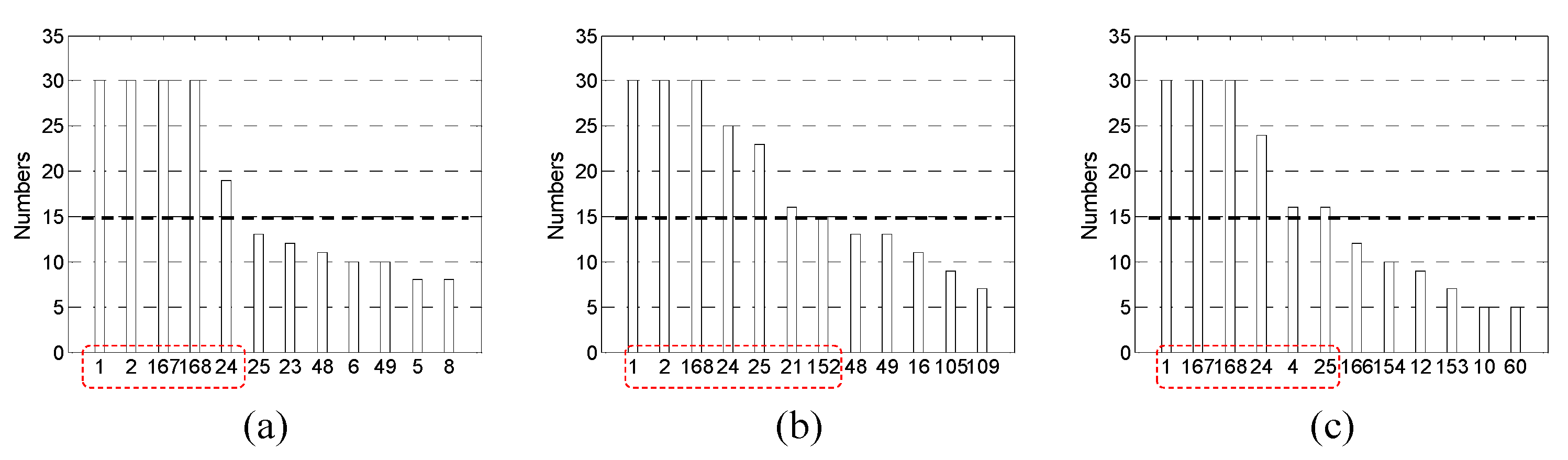Table 1 lists the results of applying Algorithm 1 for 30 times to the prepared learning dataset for predicting the loads in April 2014.

After the relevant input set X_i is joined into the union $(X=X_1\cup \cdots \cup X_{30})$, the frequency of each element in X, N_j (j = 1, …, 168), is counted. Next, N_j are arranged in descending order and the m inputs that satisfy a condition, i.e., N_j ≥ N_th, are finally selected, where N_th is the threshold value of N_j. In the hybrid methods, after removing many redundant inputs using ‘LC’ or ‘MI’, ‘GMDH’ is applied to the remaining inputs. In this study, two-thirds of the IICs were filtered by ‘LC’ or ‘MI’. 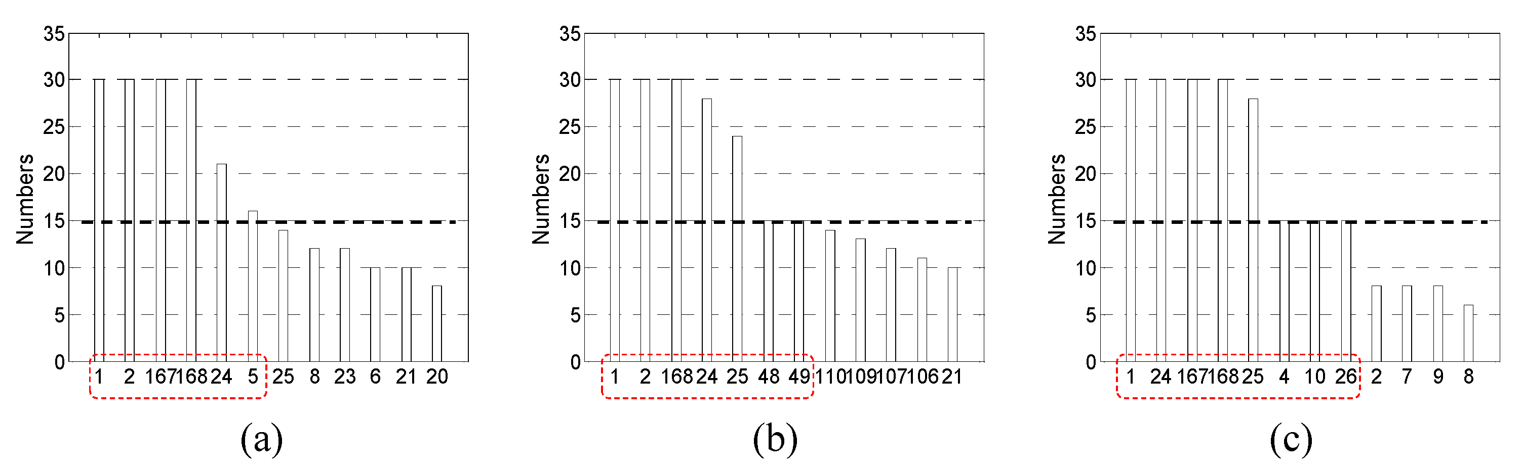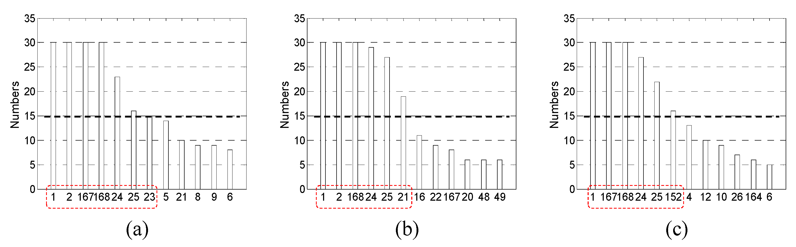Figure 8, Figure 9 and Figure 10 show the input selection results using ‘GMDH’, ‘LC + GMDH’ and ‘MI + GMDH’, respectively.

As shown in Figure 8, Figure 9 and Figure 10, the threshold value, N_th, is set as 15 and the values are marked by dashed thick solid black lines in the figures. The inputs for which N_j is greater than or equal to N_th, i.e., N_j ≥ N_th, are enclosed within dashed red lines.

Table 2. Significant inputs (SIs) selected for each validation month using the five methods: ‘LC’, ‘MI’, ‘GMDH’, ‘LC + GMDH’ and ‘MI + GMDH’. The IICs and output are {φ_t−d+1, d = 1, 2, …, 168} and φ_t+1, respectively.

Validation Month	Method	Set of Selected SIs	No.
April 2014	‘LC’	{φt−d+1|d = 1, 2, 166, 167, 168}	5
	‘MI’	{φt−d+1|d = 1, 2, 167, 168}	4
	‘GMDH’	{φt−d+1|d = 1, 2, 24, 167, 168}	5
	‘LC + GMDH’	{φt−d+1|d = 1, 2, 5, 24, 167, 168}	6
	‘MI + GMDH’	{φt−d+1|d = 1, 2, 23, 24, 25, 167, 168}	7
July 2014	‘LC’	{φt−d+1|d = 1, 2, 166, 167, 168}	5
	‘MI’	{φt−d+1|d = 1, 2, 24, 167, 168}	5
	‘GMDH’	{φt−d+1|d = 1, 2, 21, 24, 25, 152, 168}	7
	‘LC + GMDH’	{φt−d+1|d = 1, 2, 24, 25, 48, 49, 168}	7
	‘MI + GMDH’	{φt−d+1|d = 1, 2, 21, 24, 25, 168}	6
November 2014	‘LC’	{φt−d+1|d = 1, 2, 166, 167, 168}	5
	‘MI’	{φt−d+1|d = 1, 24, 167, 168}	4
	‘GMDH’	{φt−d+1|d = 1, 4, 24, 25, 167, 168}	6
	‘LC + GMDH’	{φt−d+1|d = 1, 4, 10, 24, 25, 26, 167, 168}	8
	‘MI + GMDH’	{φt−d+1|d = 1, 24, 25, 152, 167, 168}	6

summarizes the SIs selected by the five methods for each validation month (i.e., April, July, and November in 2014). As listed in Table 2, the loads in the same hour during the past several days (i.e., φ_t−23 and φ_t−167) as well as several recent loads (i.e., φ_t and φ_t−1) are useful for predicting future loads.

In addition to the selected SIs listed in Table 2, we also employed binary-valued vectors used in [45], i.e., $w\in {\{0,1\}}^7$ and $h\in {\{0,1\}}^{24}$, for ELF models to keep track of the daily and weekly periodicities, where w and h are vectors of zero with a 1 in the position of the day of the week and the hour of the day for the load under consideration, respectively.

5.3. Forecasting Results

After conducting the input selection procedures, ν-SVR learning was carried out with the SIs and binary-valued vectors, w and h. For example, when the load demand during April 2014 was predicted with ‘LC’, the input vector for ν-SVR corresponds to x = [φ_t, φ_t−1, φ_t−165, φ_t−166, φ_t−167, w_t+1, h_t+1]^T. In this paper, we used LIBSVM [46] to implement ν-SVR. The accuracy of the ELF was measured using six performance indices, which were also employed in [2,3], i.e., mean absolute percentage error (MAPE), symmetric mean absolute percentage error (SMAPE), mean absolute error (MAE), normalized mean squared error (NMSE), relative error percentage (REP) and magnitude of maximum error (MME). In the following, we only present the results of the performance comparisons using MAPE, which is defined as

$$\mathrm{MAPE}=\frac{1}{N}{\displaystyle \sum _{i=1}^N\frac{\left|A_i-F_i\right|}{A_i}}\times 100,$$

(15)

where A_i and F_i are the actual and predicted values for the ith validation dataset, respectively, and N is the number of validation dataset. The performance comparisons using the other indices are presented in Appendix B.

Table 3. Mean absolute percentage error (MAPE) values of each validation month and the overall values. The last three rows indicate the overall MAPE values for three validation months and the second column represents the prediction horizons, i.e., H = 1, H = 24, and H = 168, which correspond to one-hour, one-day and one-week-ahead forecasting, respectively.

Validation Month	H	‘LC’	‘MI’	‘GMDH’	‘LC + GMDH’	‘MI + GMDH’
April 2014	1	0.559	0.545	0.526 +	0.531	0.496 *
	24	1.361	1.321	1.252 +	1.265	1.162 *
	168	1.675	1.656	1.604 +	1.604	1.559 *
July 2014	1	0.459	0.474	0.457 +	0.478	0.438 *
	24	1.759	1.576	1.514 +	1.678	1.434 *
	168	2.108	1.900 +	1.925	2.025	1.834 *
November 2014	1	0.582	0.556	0.544 +	0.548	0.534 *
	24	2.047	1.666 +,*	1.725	1.728	1.676
	168	2.485	2.301 +	2.371	2.393	2.293 *
Overall	1	0.532	0.524	0.508 +	0.519	0.489 *
	24	1.723	1.522	1.497 +	1.558	1.424 *
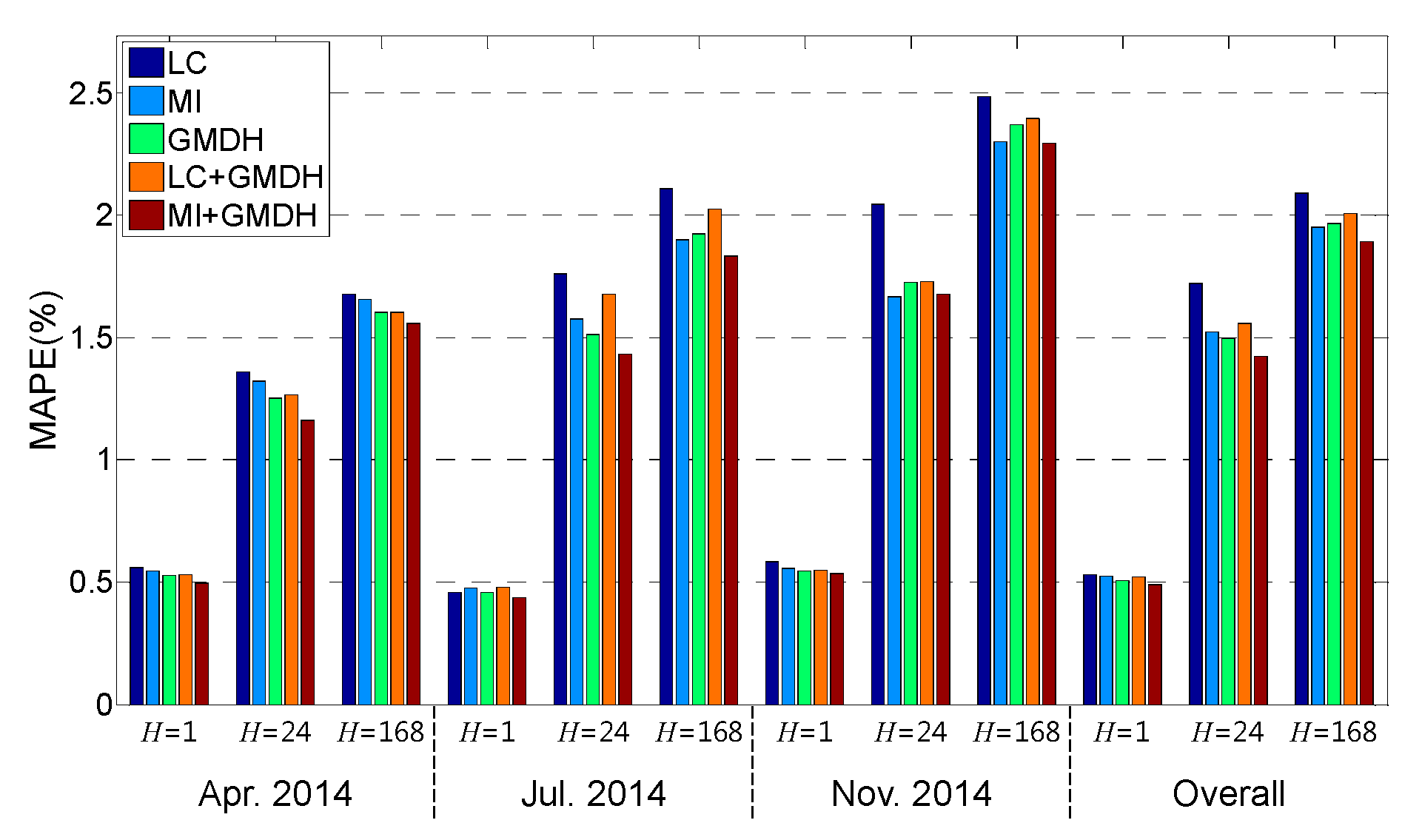
	168	2.090	1.952 +	1.966	2.008	1.894 *

and Figure 11 illustrate the MAPE values of each validation month and the overall values for five input selection methods.

In Table 3, the best entries among ‘LC’, ‘MI’ and ‘GMDH’ are indicated by the superscript plus sign and the best entries among the five input selection methods are highlighted by the superscript asterisk. When H = 1, i.e., in the case of one-hour ahead forecasting, MAPE values of every validation month are similar to each other; but when H = 24 and 168, they are quite different. This can be attributed to the fact that load variations in July and November are higher than those in April because of seasonal effects; it can be observed that MAPE values for multi-step ahead forecasting in July and November are larger than those in April.

As illustrated in Table 3 and Figure 11, ‘GMDH’ shows the best prediction performance among ‘LC’, ‘MI’, and ‘GMDH’ in terms of the overall MAPE, except for one-week-ahead forecasting. Among the five methods, ‘MI + GMDH’ shows the best forecasting performance, except for the one-day-ahead forecast for November 2014. Let us look at how much ‘MI + GMDH’ improves the overall MAPE compared with the other methods. For one-hour-ahead forecasting, the percentage improvements with ‘MI + GMDH’ are 8.19%, 6.79%, 3.80%, and 5.72% compared with the four methods, respectively. For one-day and one-week-ahead forecasting, ‘MI + GMDH’ improves the overall MAPE compared with the other methods by 17.35%, 6.45%, 4.91%, and 8.64%, and by 9.34%, 2.93%, 3.64%, and 5.65%, respectively. 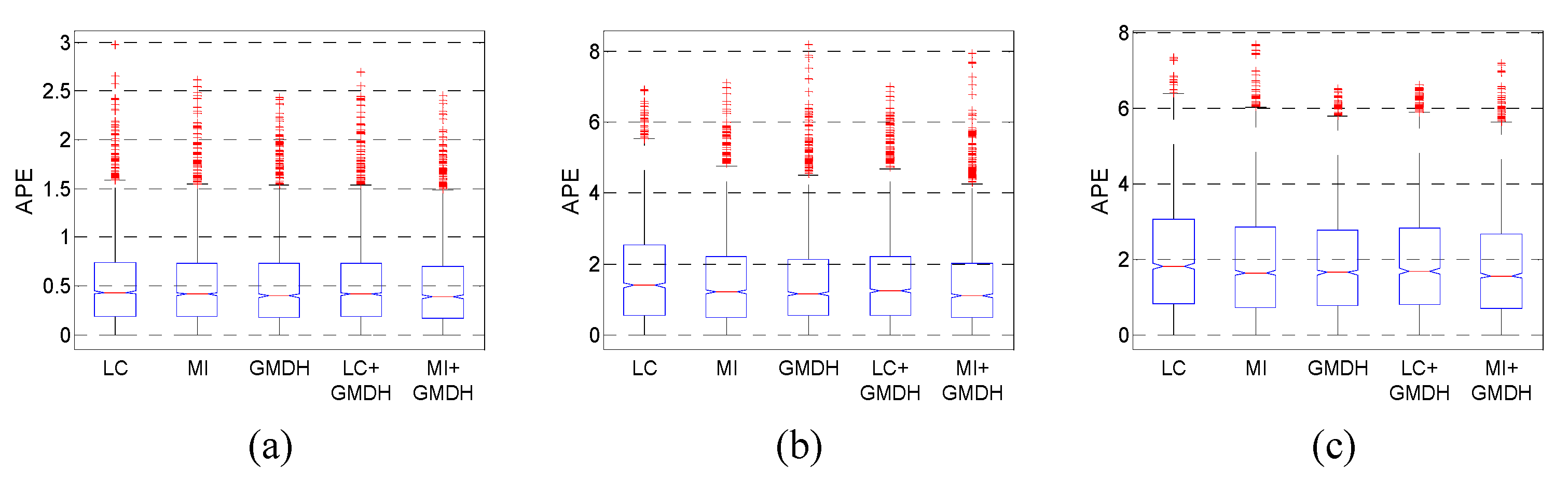Figure 12 shows box plots of the overall absolute percentage errors. As shown in Figure 12, ‘MI + GMDH’ exhibits superior performance compared with the other methods. 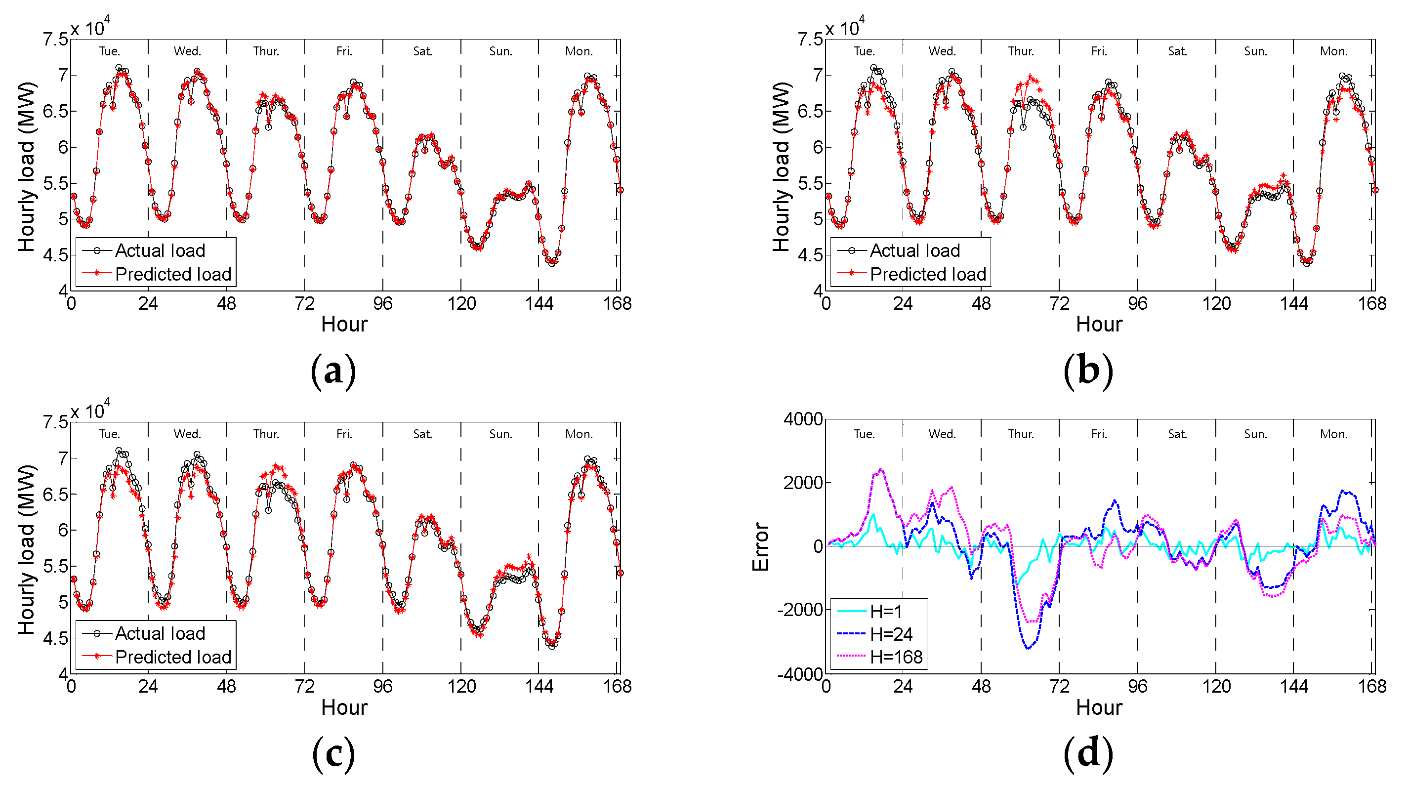Figure 13 shows examples of the actual and predicted load curves obtained using ‘MI + GMDH’ and ν-SVR. Due to space constraints, the load curves for the other validation months and periods are not presented. In Figure 13, the load values predicted by ‘MI + GMDH’ and ν-SVR are very similar to the actual values. 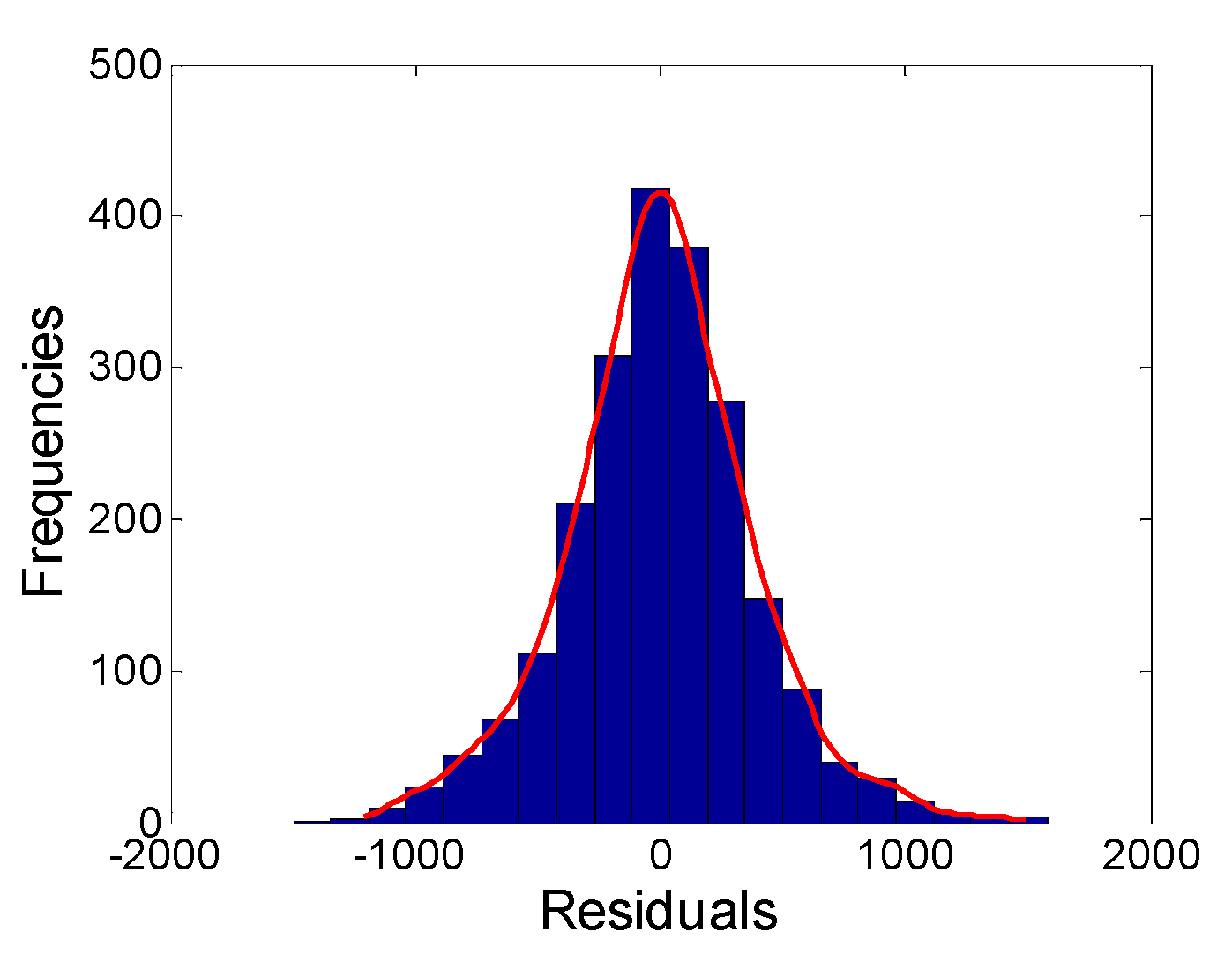Figure 14 shows a histogram of illustrating the one-hour-ahead prediction errors by ‘MI + GMDH’ and ν-SVR for July 2014.

As shown in Figure 14, the errors are centered symmetrically on zero and there are no severe outliers. Figure 15 illustrates the results of linear regression analysis between the actual and predicted load values by ‘MI + GMDH’ and ν-SVR for July 2014.

The results for the other validation months are not presented due to space limitations. In Figure 15, the X and Y axes correspond to the actual and predicted load values, respectively, the black circles are scatter plots of the data points, i.e., (X, Y), and the dashed black lines and thick solid blue lines indicate the straight lines, Y = X, and the best linear regression lines, respectively. The r² values presented above the figures represent the relationships between X and Y. A value close to 1 indicates that X and Y have a strong linear relationship. As illustrated in Figure 15, we can confirm that there are strong linear relationships between the actual and predicted load values.

6. Discussion

Based on the experimental results presented in Section 5, we can highlight several key findings. Let us begin with the comparisons between the filter methods (i.e., ‘LC’ and ‘MI’) and ‘GMDH’. At one-hour and one-day ahead forecasting, ‘GMDH’ performed better than the filter methods in terms of the overall MAPE. There are two main reasons for the improved performance of ‘GMDH’: (1) ‘GMDH’ can capture many-to-one nonlinear relationships between inputs and output via hierarchical network structure, whereas ‘LC’ or ‘MI’ can only capture one-to-one linear or nonlinear relationships; and (2) unlike filter methods that select SIs based on statistical RF, the prediction accuracy (i.e., CEC) is employed as an input selection criterion in ‘GMDH’.

Second, we consider the performance comparisons between ‘GMDH’ and the hybrid methods. In all cases, ‘MI + GMDH’ obtained the best forecasts in terms of the overall MAPE. The load series has nonlinear characteristics and ν-SVR with a nonlinear kernel (i.e., RBF kernel) was used for the prediction models, so the hybrid method that combines ‘MI’ with ‘GMDH’ performed better. The prediction results of ‘LC + GMDH’ were poor compared with ‘GMDH’ alone because LC-based filtering procedure may remove the inputs with weak linear but strong nonlinear relationships with the output.

Finally, let us discuss the performance of the five methods in terms of their computational time requirements.

Table 4. Computational time required by the five input selection methods for April 2014.

Input Selection Methods	Time
‘LC’	9.863 s
‘MI’	3402.265 s
‘GMDH’	1483.911 s
‘LC + GMDH’	189.622 s
‘MI + GMDH’	3572.328 s

lists the computational time required by each input selection method for April 2014.

The learning dataset is composed of 2904 input-output pairs and 168 IICs comprise the input part for each pair. The computer used to measure the computational time had 8 GB of RAM and a 2.8 GHz quad-core CPU. The result shows clearly that the computational efficiency of ‘GMDH’ is higher than that of ‘MI’. The computational time required by ‘LC + GMDH’ is much less than that of ‘GMDH’ alone because the number of inputs handled by ‘GMDH’ is reduced to one-third of the IICs by the LC-based filtering procedure.

7. Conclusions

In this study, we proposed a new input selection procedure, which combines GMDH with a bootstrap method for SVR-based short-term hourly load forecasting. After constructing GMDH networks many times under the same experimental conditions, the inputs that remain frequently in the input layers were finally selected as SIs. The networks were constructed several times because each relevant input is different due to the random division of the learning dataset. Indeed, only constructing a single network could yield biased input selection results. In experimental assessments, we employed LC- and MI-based filter methods for comparison, and also verified the performance of two hybrid methods. In total, five input selection methods were examined in this study. To illustrate the performance of the proposed method, an hourly load dataset from South Korea was used and the one-hour, one-day and one-week-ahead forecasting performances were compared.

The experimental results showed that the proposed method can select SIs in an effective manner. The forecasting performance of the proposed method (i.e., ‘GMDH’) was better than that of the LC- and MI-based filter methods. To be specific, in one-hour, one-day, and one-week ahead forecasts, ‘GMDH’ improves the overall MAPE values by 0.024, 0.226, and 0.124, respectively, over ‘LC’. Although the overall MAPE with H = 168 worsens by 0.014, when H = 1 and 24, ‘GMDH’ improves the overall MAPE values by 0.016 and 0.025, respectively, compared with ‘MI’. In addition, the computational efficiency of the proposed method was higher than that of the MI-based filter method. Among the five methods, ‘MI + GMDH’ achieved the best prediction accuracy. When H = 1, 24, and 168, ‘MI + GMDH’ outperforms ‘GMDH’, with 0.019, 0.073, and 0.072, respectively, improvements in overall MAPE values.

Let us summarize the main reasons for the improved performance of the proposed method. First, the proposed method can perform input selection by capturing many-to-one nonlinear relationships between potential inputs and output via the hierarchical structure of the GMDH network. Second, compared with the filter methods, the prediction accuracy (i.e., CEC) is employed as a selection criterion, which improves the prediction performance. Finally, SIs are selected by constructing GMDH networks many times, thereby facilitating more robust input selections.

In future research, the proposed method will be applied to hourly load forecasting on special days and daily peak load forecasting. Moreover, the proposed method can be used in various real-world applications such as financial time-series analysis, process monitoring, and nonlinear function approximations.