A dq-Domain Impedance Measurement Methodology for Three-Phase Converters in Distributed Energy Systems

 , , , ,
Abstract
1. Introduction
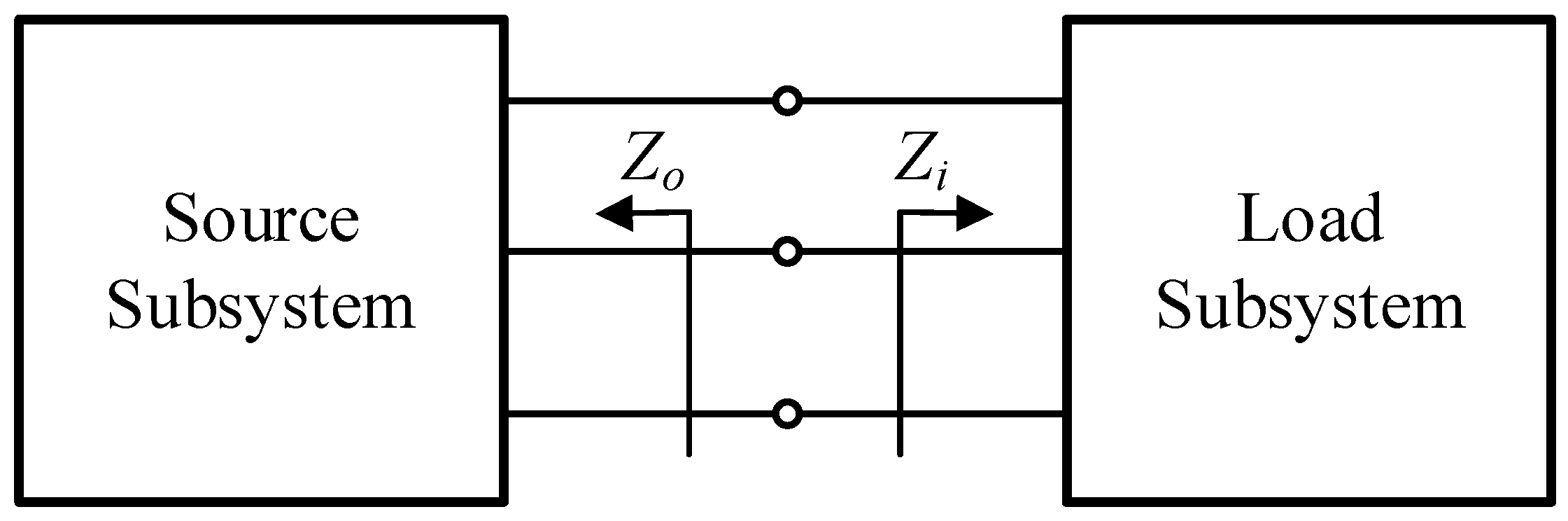
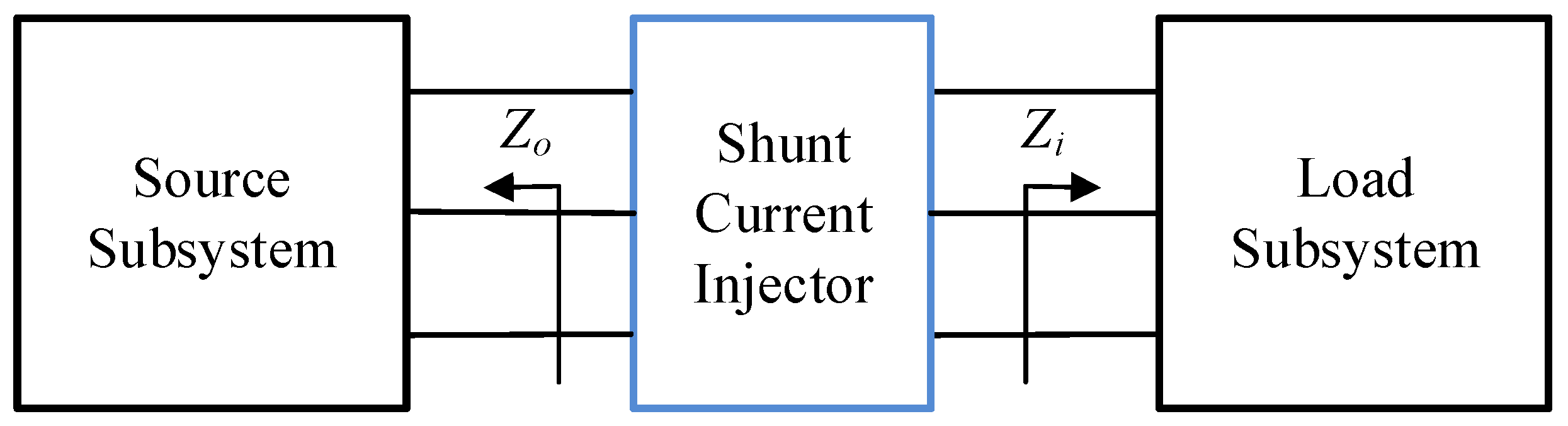
2. Impedance Measurement Methodology Using Shunt Current Injection Approach
- is the source subsystem’s output impedance;
- is the load subsystem’s input admittance;
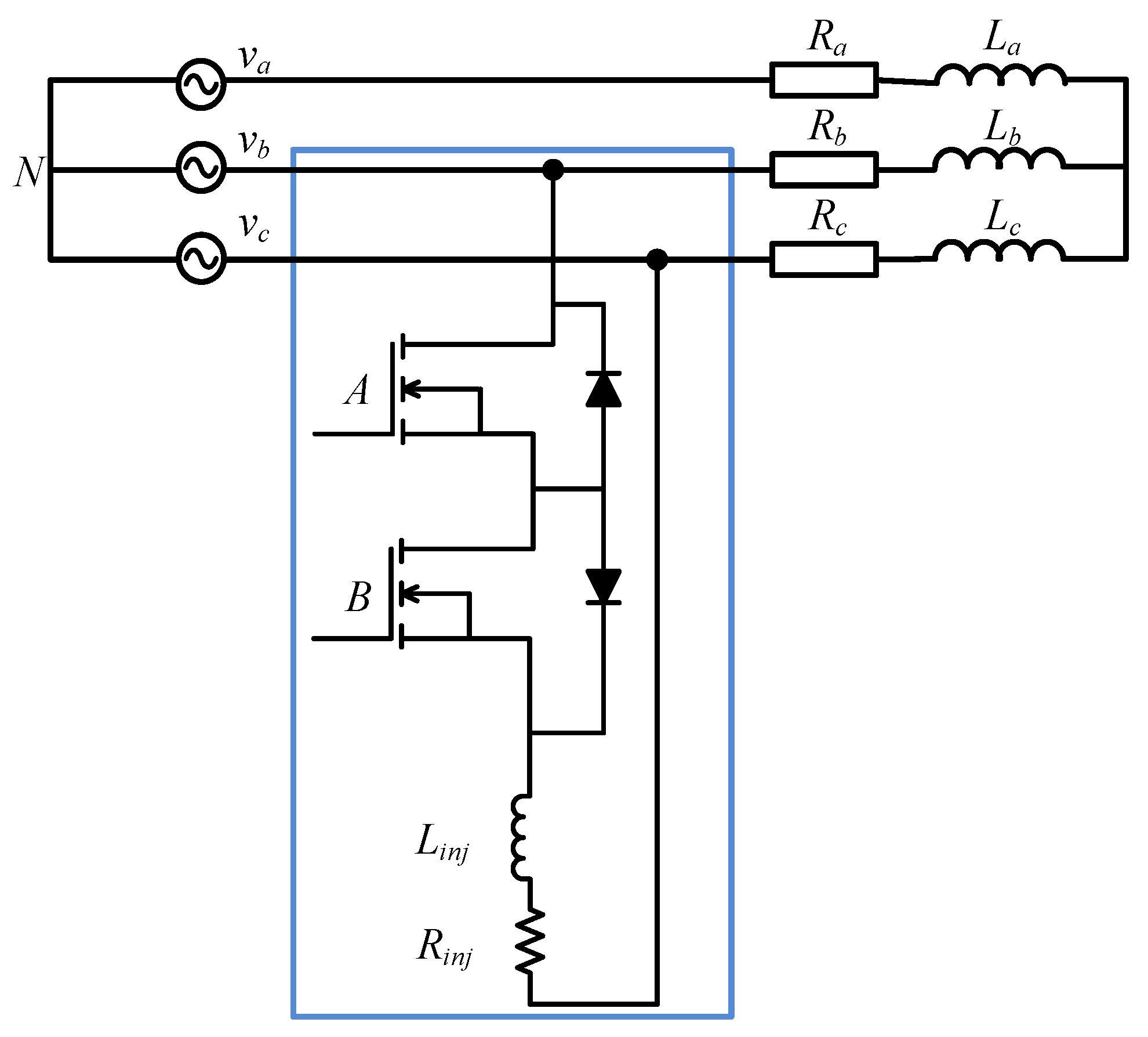
- is the three-phase source voltage;
- is the resistor;
- is the inductor;
- is the injection resistor;
- is the injection inductor;
- is the power metal-oxide-semiconductor field-effect transistor (MOSFET).
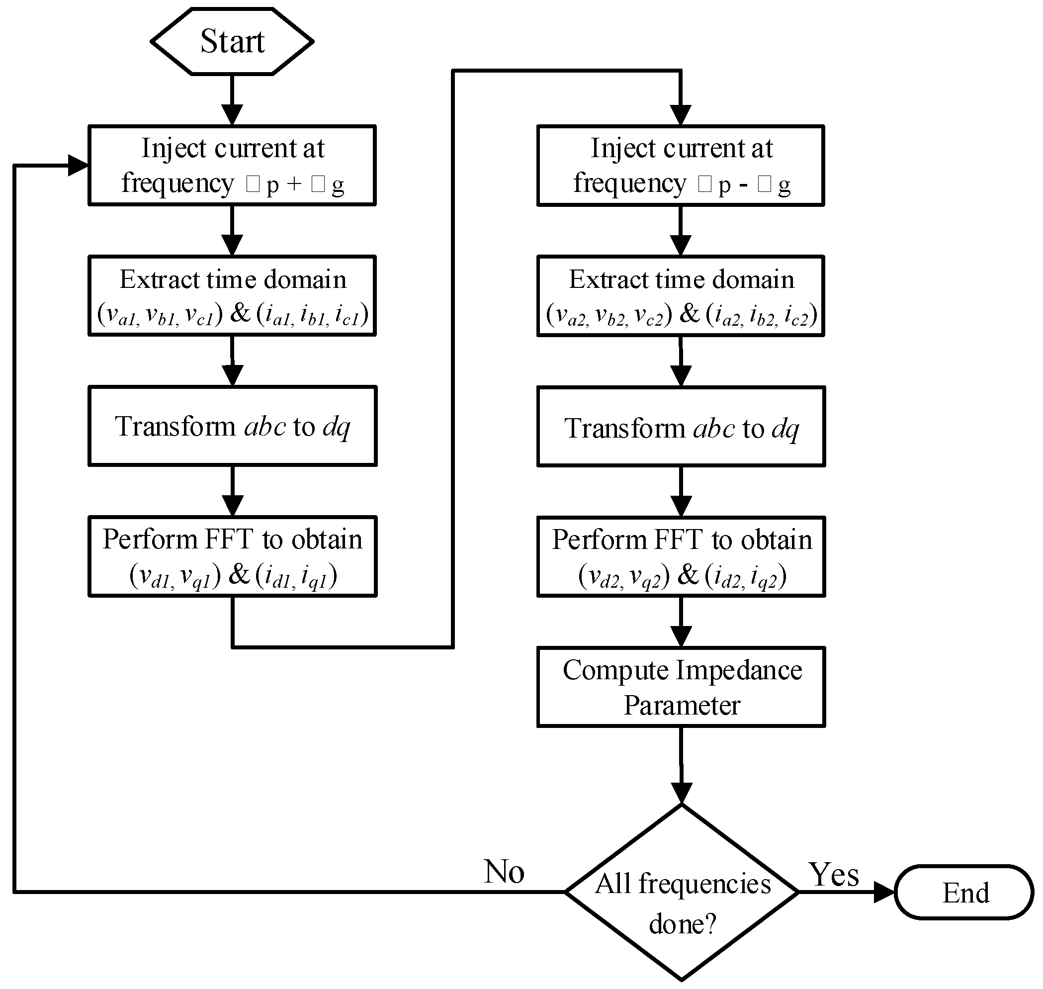
3. Impedance Measurement Methodology in the -Domain
3.1. Measurements of and
3.2. Measurements of and
3.3. Perturbations for and
3.4. Perturbations for and
4. Impedance Measurement Set-Up
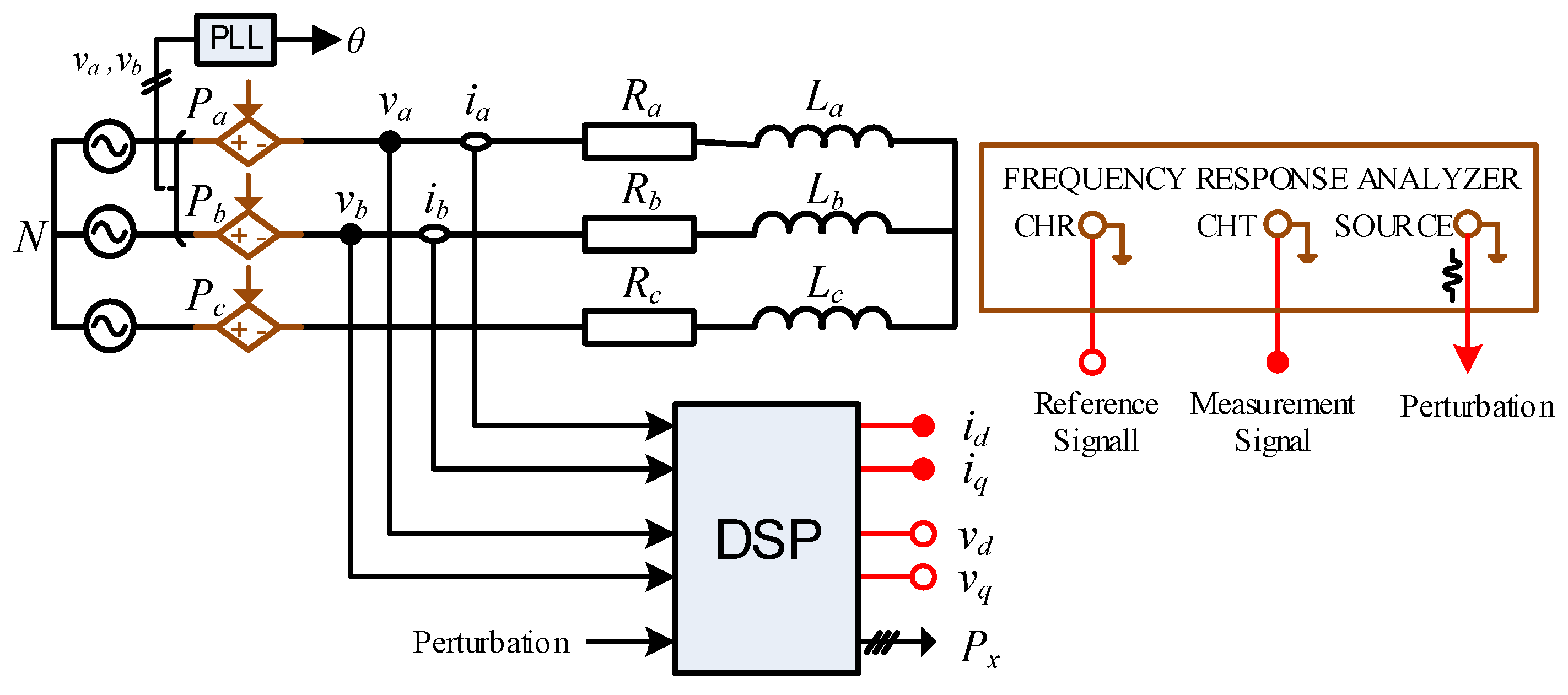
4.1. Measurement Set-Up
- is the three-phase source voltage;
- is the three-phase source current;
- is the perturbation signal;
- is the resistor;
- is the inductor;
- is the -domain voltage;
- is the -domain current.
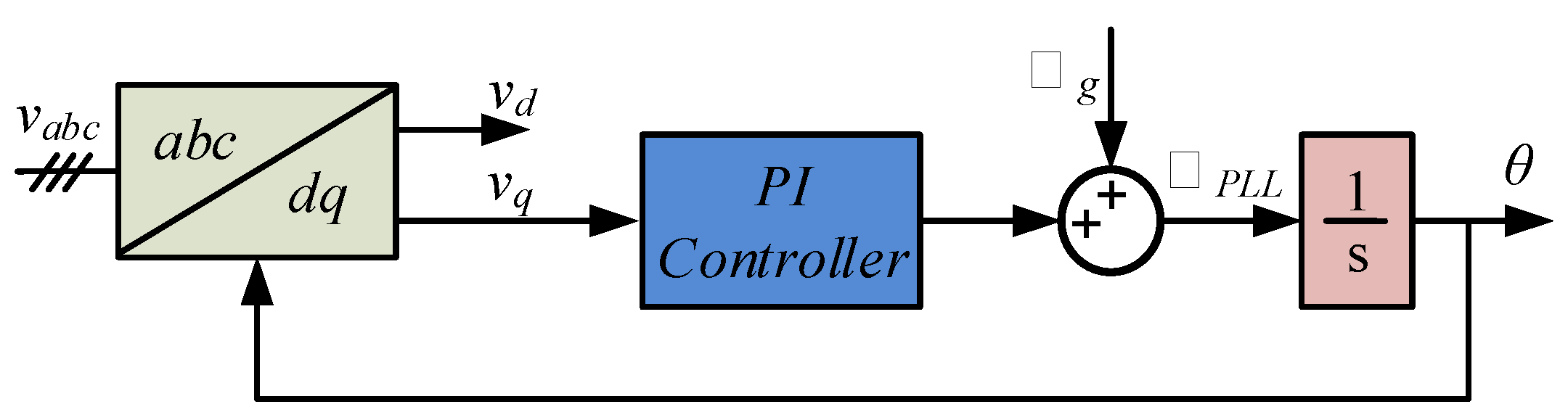
4.2. Phase-Locked Loop
5. Impedance Measurement Results
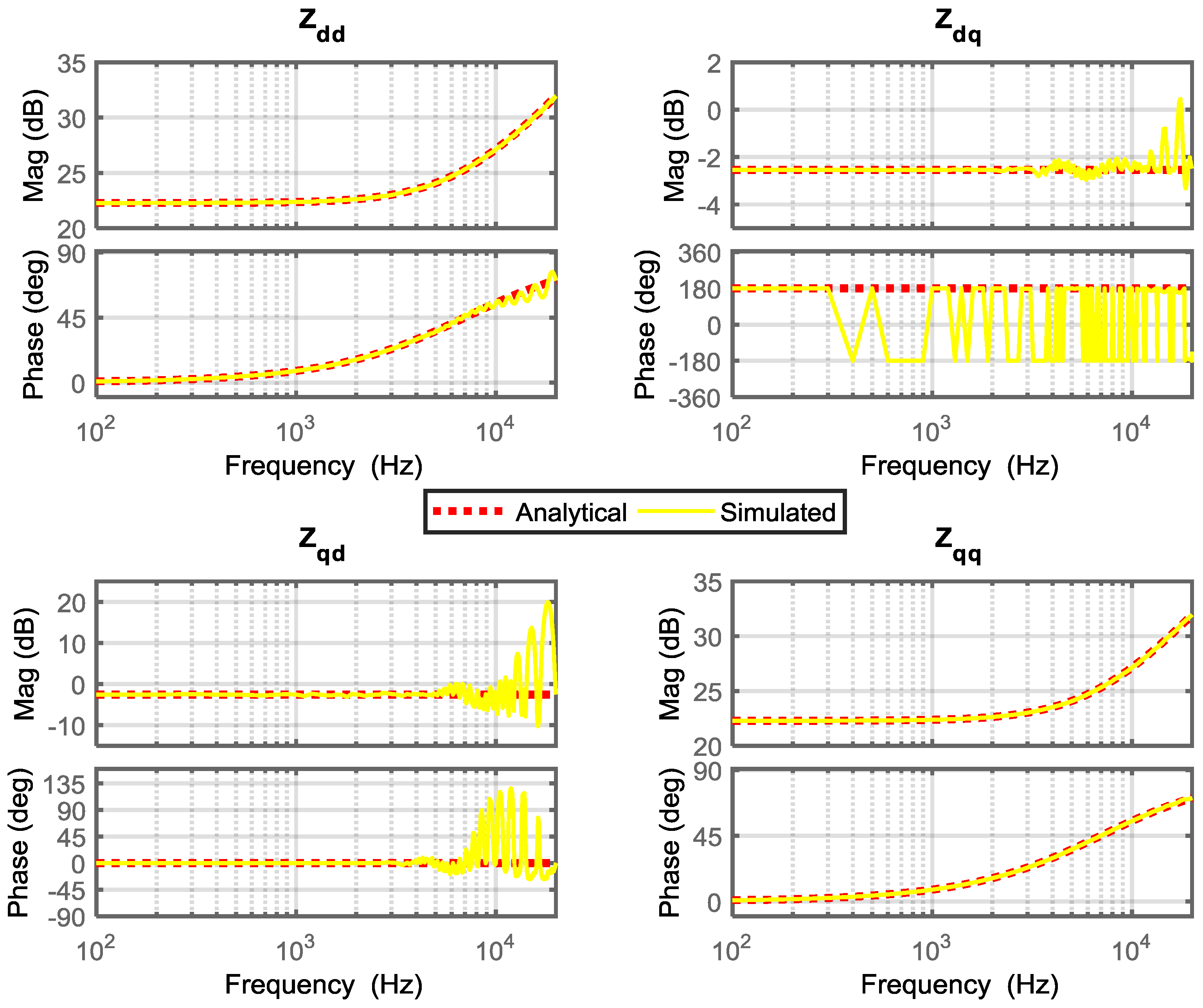
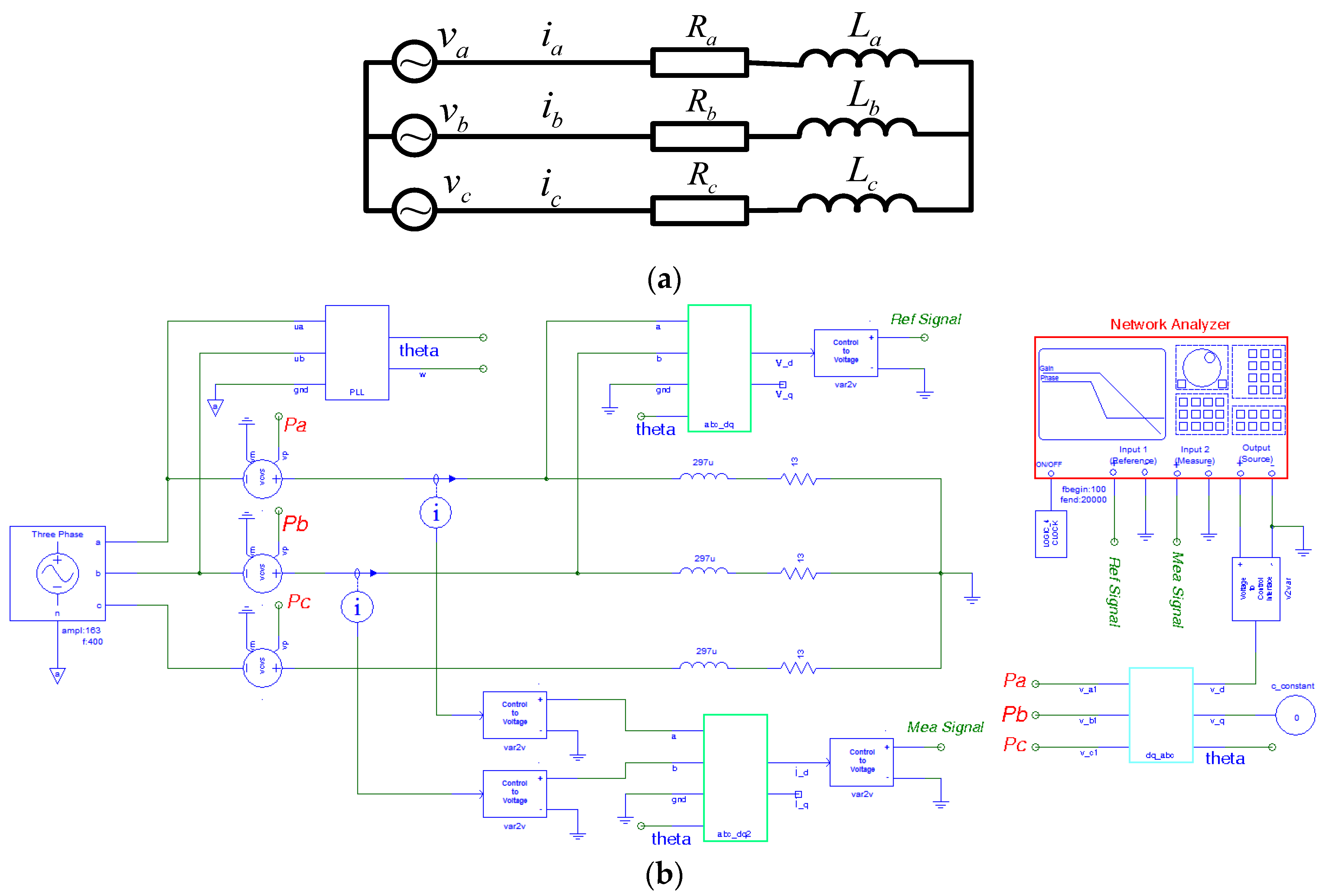
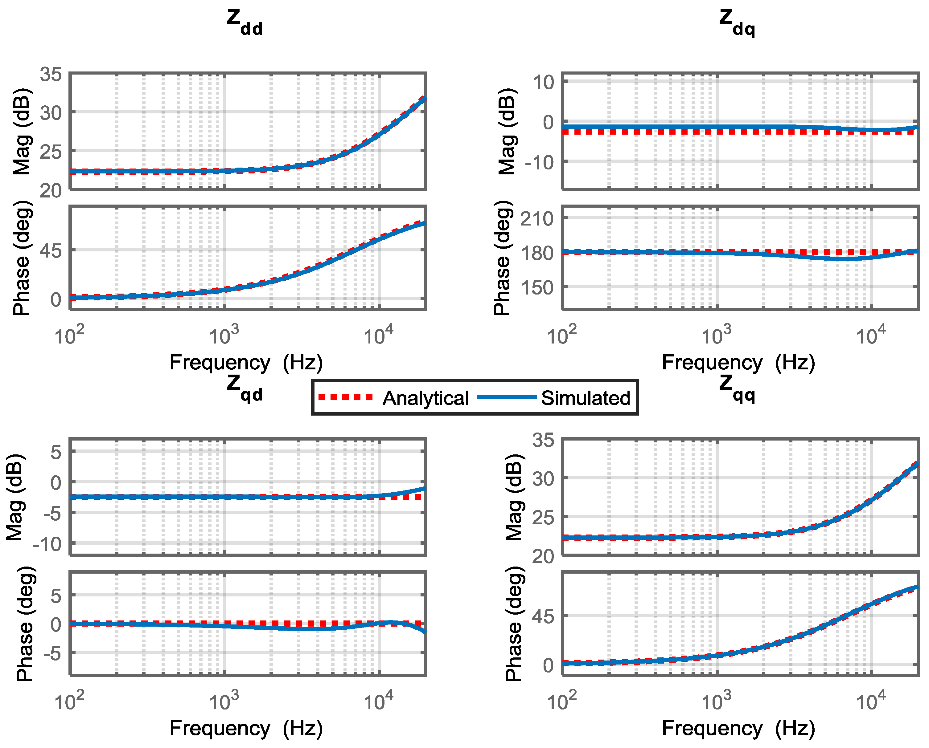
5.1. Simulation Results
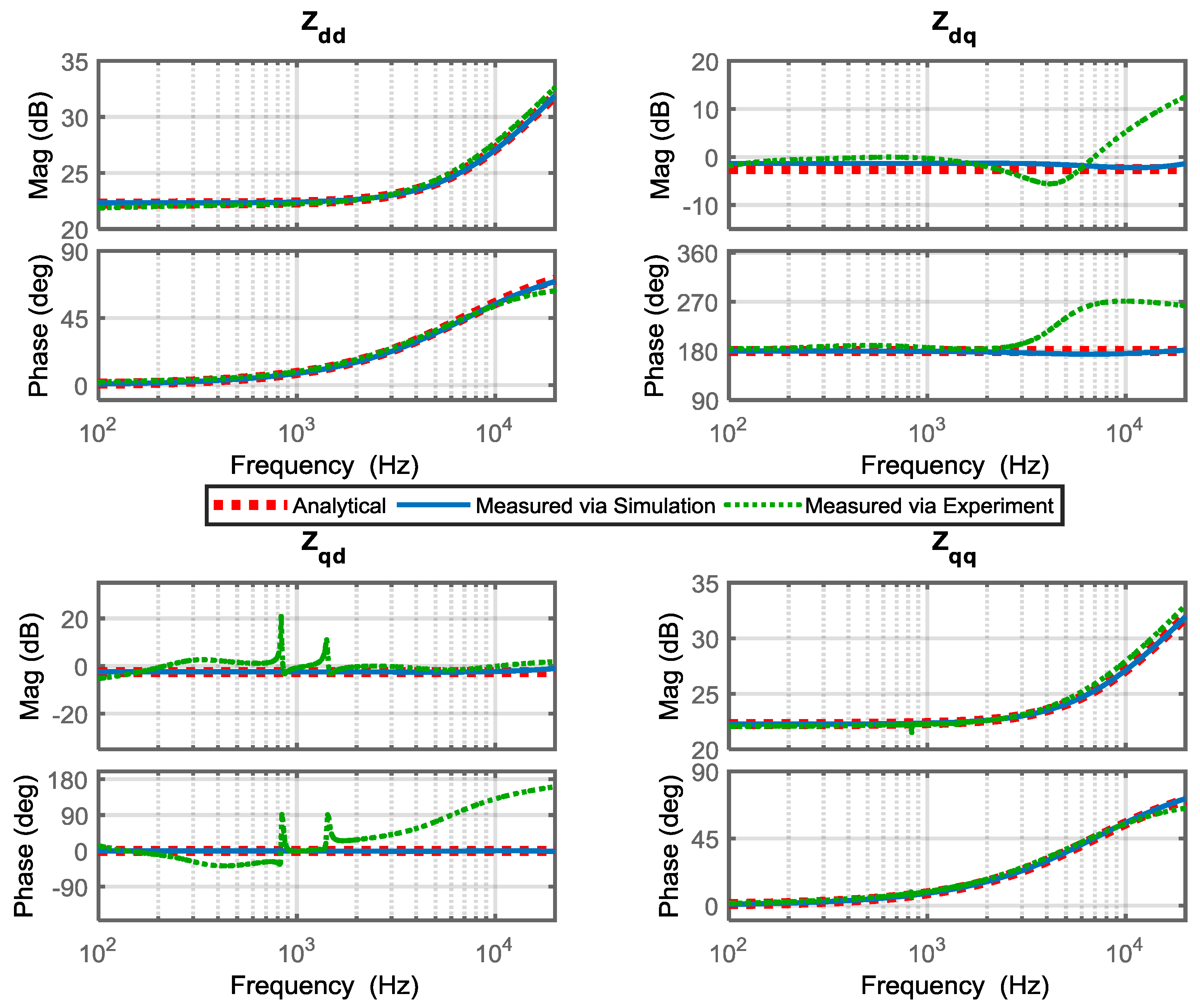
5.2. Experimental Results
6. Conclusions
Author Contributions
Funding
Conflicts of Interest
References
- Wen, B.; Burgos, R.; Boroyevich, D.; Mattavelli, P.; Shen, Z. AC Stability Analysis and dq Frame Impedance Specifications in Power-Electronics-Based Distributed Power Systems. IEEE J. Emerg. Sel. Top. Power Electron. 2017, 5, 1455–1465. [Google Scholar] [CrossRef]
- Bose, B.K. Global Energy Scenario and Impact of Power Electronics in 21st Century. IEEE Trans. Ind. Electron. 2013, 60, 2638–2651. [Google Scholar] [CrossRef]
- Nefedov, E.; Sierla, S.; Vyatkin, V. Internet of Energy Approach for Sustainable Use of Electric Vehicles as Energy Storage of Prosumer Buildings. Energies 2018, 11, 2165. [Google Scholar] [CrossRef]
- Harighi, T.; Bayindir, R.; Padmanaban, S.; Mihet-Popa, L.; Hossain, E. An Overview of Energy Scenarios, Storage Systems and the Infrastructure for Vehicle-to-Grid Technology. Energies 2018, 11, 2174. [Google Scholar] [CrossRef]
- Saponara, S.; Ciarpi, G. IC Design and Meaasuremetn of an Inductorless 48V DC/DC Converter in Low-Cost CMOS Technology Facing Harsh Environments. IEEE Trans. Circuits Syst. I 2018, 65, 380–393. [Google Scholar] [CrossRef]
- Aldhaheri, A.; Etemadi, A. Impedance Decoupling in DC Distributed Systems to Maintain Stability and Dynamic Performance. Energies 2017, 10, 470. [Google Scholar] [CrossRef]
- Mehrasa, M.; Adabi, M.E.; Pouresmaeil, E.; Adabi, J.; Jorgensen, B.N. Direct Lyapunov Control (DLC) Technique for Distributed Generation (DG) Technology. Electr. Eng. 2014, 96, 309–321. [Google Scholar] [CrossRef]
- Mehrasa, M.; Pouresmaeil, E.; Shamsodin, T.; Vechiu, I.; Catalao, J.P.S. Novel Control Strategy for Modular Multilevel Converters Based on Differential Flatness Theroy. IEEE J. Emerg. Sel. Top. Power Electron. 2018, 6, 888–897. [Google Scholar] [CrossRef]
- Mehrasa, M.; Sharifzadeh, M.; Sheikholeslami, A.; Pouresmaeil, E.; Catalao, J.P.S.; Al-Haddad, K. A Control based on Upper and Lower’s Arms Modulation Functions of MMC in HVDC Applications. In Proceedings of the IEEE International Conference on Industrial Technology (ICIT), Lyon, France, 20–22 February 2018. [Google Scholar]
- Miceli, R.; Schettino, G.; Viola, F. A Novel Computational Approach for Harmonic Mitigation in PV Systems with Single-Phase Five-Level CHBMI. Energies 2018, 11, 2100. [Google Scholar] [CrossRef]
- Polanco Vasquez, L.O.; Carreño Meneses, C.A.; Pizano Martínez, A.; López Redondo, J.; Pérez García, M.; Álvarez Hervás, J.D. Optimal Energy Management within a Microgrid: A Comparative Study. Energies 2018, 11, 2167. [Google Scholar] [CrossRef]
- Liu, F.; Liu, J.; Zhang, H.; Xue, D.; Dou, Q. Comprehensive study about stability issues of multi-module distributed system. In Proceedings of the International Power Electronics Conference (IPEC), Hiroshima, Japan, 18–21 May 2014. [Google Scholar]
- Rygg, A.; Molinas, M. Apparent Impedance Analysis: A Small-Signal Method for Stability Analysis of Power Electronic-Based Systems. IEEE J. Emerg. Sel. Top. Power Electron. 2017, 5, 1474–1486. [Google Scholar] [CrossRef]
- Jaksic, M.; Shen, Z.; Cvetkovic, I.; Boroyevich, D.; Burgos, R.; DiMarino, C.; Chen, F. Medium-Voltage Impedance Measurement Unit for Assessing the System Stability of Electric Ships. IEEE Trans. Energy Convers. 2017, 32, 829–841. [Google Scholar] [CrossRef]
- Lissandron, S.; Santa, L.D.; Mattavelli, P.; Wen, B. Experimental validation for impedance-based small-signal stability analysis of single phase interconnected power systems with grid-feeding inverters. IEEE J. Emerg. Sel. Top. Power Electron. 2016, 4, 103–115. [Google Scholar] [CrossRef]
- Amin, M.; Ardal, A.; Molinas, M. Self-synchronization of wind farm in an MMC-based HVDC system: A stability investigation. IEEE Trans. Energy Convers. 2017, 32, 458–470. [Google Scholar] [CrossRef]
- Liu, Z.; Liu, J.; Bao, W.; Zhao, Y. Infinity-norm of Impedance-based Stability Criterion for Three-phase AC Distributed Power Systems with Constant Power Loads. IEEE Trans. Power Electron. 2015, 30, 3030–3043. [Google Scholar] [CrossRef]
- Suntio, T.; Viinamaki, J.; Jokipii, J.; Messo, T.; Kuperman, A. Dynamic Characterization of Power Electronic Interfaces. IEEE J. Emerg. Sel. Top. Power Electron. 2014, 2, 949–961. [Google Scholar] [CrossRef]
- Sun, J. Small-signal Methods for AC Distributed Power Systems—A Review. IEEE Trans. Power Electron. 2009, 24, 2545–2554. [Google Scholar]
- Wen, B.; Boroyevich, D.; Mattavelli, P.; Zhiyu, S.; Burgos, R. Experimental verification of the generalized Nyquist stability criterion for balanced three-phase ac systems in the presence of constant power loads. In Proceedings of the IEEE Energy Conversion Congress and Exposition (ECCE), Raleigh, NC, USA, 15–20 September 2012. [Google Scholar]
- Rygg, A.; Molinas, M.; Zhang, C.; Cai, X. A modified sequence domain impedance definition and its equivalence to the dq-domain impedance definition for the stability analysis of AC power electronic systems. IEEE J. Emerg. Sel. Top. Power Electron. 2016, 4, 1383–1396. [Google Scholar] [CrossRef]
- Cao, W.; Ma, Y.; Wang, F. Sequence-impedance-based harmonic stability analysis and controller parameter design of three-phase inverter based multi bus AC power systems. IEEE Trans. Power Electron. 2016, 32, 7674–7693. [Google Scholar] [CrossRef]
- Xu, L.; Fan, L.; Miao, Z. DC impedance-model-based resonance analysis of a VSC–HVDC system. IEEE Trans. Power Deliv. 2015, 30, 1221–1230. [Google Scholar] [CrossRef]
- Tarateeraseth, V.; See, K.-Y.; Canavero, F.G.; Chang, R.W.-Y. Systematic Electromagnetic Interference Filter Design Based on Information from in-Circuit Impedance Measurements. IEEE Trans. Electromagn. Compat. 2010, 52, 588–598. [Google Scholar] [CrossRef]
- Liu, Z.; Liu, J.; Hou, X.; Dou, Q.; Xue, D.; Liu, T. Output impedance modeling and stability prediction of three-phase paralleled inverters with master-slave sharing scheme based on terminal characteristics of individual inverters. IEEE Trans. Power Electron. 2016, 31, 5306–5320. [Google Scholar] [CrossRef]
- Ali, H.; Zheng, X.; Wu, X.; Khan, S.; Saad, M. Frequency response measurements of dc-dc buck converter. In Proceedings of the IEEE International Conference on Information and Automation (ICIA), Lijiang, China, 8–10 August 2015. [Google Scholar]
- Zheng, X.; Ali, H.; Wu, X.; Zaman, H.; Khan, S. Non-Linear Behavioral Modeling for DC-DC Converters and Dynamic Analysis of Distributed Energy Systems. Energies 2017, 10, 63. [Google Scholar] [CrossRef]
- Shen, Z.; Jaksic, M.; Mattavelli, P.; Boroyevich, D.; Verhulst, J.; Belkhayat, M. Design and implementation of three-phase AC impedance measurement unit (IMU) with series and shunt injection. In Proceedings of the 28th Annual IEEE Applied Power Electronics Conference and Exposition (APEC), Long Beach, CA, USA, 17–21 March 2013. [Google Scholar]
- Huang, J.; Corzine, K.A.; Belkhayat, M. Small-Signal Impedance Measurement of Power-Electronics-Based AC Power Systems Using Line-to-Line Current Injection. IEEE Trans. Power Electron. 2009, 24, 445–455. [Google Scholar] [CrossRef]
- Francis, G.; Burgos, R.; Boroyevich, D.; Wang, F.; Karimi, K. An algorithm and implementation system for measuring impedance in the d-q domain. In Proceedings of the IEEE Energy Conversion Congress and Exposition (ECCE), Phoenix, Arizona, AZ, USA, 17–22 September 2011. [Google Scholar]
- Gu, H.; Guo, X.; Wang, D.; Wu, W. Real-time grid impedance estimation technique for grid connected power converters. In Proceedings of the IEEE International Symposium on Industrial Electronics, Hangzhou, China, 28–31 May 2012. [Google Scholar]
- Martin, D.; Santi, E.; Barkley, A. Wide bandwidth system identification of AC system impedances by applying perturbations to an existing converter. In Proceedings of the Energy Conversion Congress and Exposition, Phoenix, AZ, USA, 17–22 September 2011. [Google Scholar]
- Dou, Q.; Liu, Z.; Liu, J.; Boa, W. A novel impedance measurement method for three-phase power electronic systems. In Proceedings of the 9th International Conference on Power Electronics and ECCE Asia (ICPE-ECCE Asia), Seoul, Korea, 1–5 June 2015. [Google Scholar]
- MathWorks. Available online: http://www.mathworks.com (accessed on 3 September 2017).
- Arricibita, D.; Marroya, L.; Barrios, E.L. Simple and robust PLL algorithm for accurate phase tracking under grid disturbances. In Proceedings of the IEEE 18th Workshop on Control and Modeling of Power Electronics (COMPEL), Stanford, CA, USA, 9–12 July 2017. [Google Scholar]
- Saber Sketch. Available online: https://www.synopsys.com/verification/virtual-prototyping/saber.html (accessed on 14 August 2017).


| Parameter | Source Voltage | Source Frequency | Load Resistor | Load Inductor | Injection Resistor | Injection Inductor |
|---|---|---|---|---|---|---|
| Value | 115 | 400 | 13 | 297 | 100 | 1 |
| Parameter | Source Voltage | Source Frequency | Load Resistor | Load Inductor |
|---|---|---|---|---|
| Value | 115 | 400 | 13 | 297 |
| Parameter | Source Voltage | Source Frequency | Load Resistor | Load Inductor |
|---|---|---|---|---|
| Value | 20 | 400 | 13 | 297 |
© 2018 by the authors. Licensee MDPI, Basel, Switzerland. This article is an open access article distributed under the terms and conditions of the Creative Commons Attribution (CC BY) license (http://creativecommons.org/licenses/by/4.0/).
Share and Cite
Saad, M.; Ali, H.; Liu, H.; Khan, S.; Zaman, H.; Khan, B.M.; Kai, D.; Yongfeng, J. A dq-Domain Impedance Measurement Methodology for Three-Phase Converters in Distributed Energy Systems. Energies 2018, 11, 2732. https://doi.org/10.3390/en11102732
Saad M, Ali H, Liu H, Khan S, Zaman H, Khan BM, Kai D, Yongfeng J. A dq-Domain Impedance Measurement Methodology for Three-Phase Converters in Distributed Energy Systems. Energies. 2018; 11(10):2732. https://doi.org/10.3390/en11102732
Chicago/Turabian StyleSaad, Muhammad, Husan Ali, Huamei Liu, Shahbaz Khan, Haider Zaman, Bakht Muhammad Khan, Du Kai, and Ju Yongfeng. 2018. "A dq-Domain Impedance Measurement Methodology for Three-Phase Converters in Distributed Energy Systems" Energies 11, no. 10: 2732. https://doi.org/10.3390/en11102732
APA StyleSaad, M., Ali, H., Liu, H., Khan, S., Zaman, H., Khan, B. M., Kai, D., & Yongfeng, J. (2018). A dq-Domain Impedance Measurement Methodology for Three-Phase Converters in Distributed Energy Systems. Energies, 11(10), 2732. https://doi.org/10.3390/en11102732