Abstract
This paper investigated the effect of oxygen holdup on the current density distribution over the electrode of a vertical/horizontal electrolysis cell with a two-dimensional Eulerian–Eulerian two-phase flow model in the acrylonitrile (AN) electrolytic adiponitrile (ADN) process. The physical models consisted of a vertical/horizontal electrolysis cell 10 mm wide and 600 mm long. The electrical potential difference between the anode and cathode was fixed at 5 V, which corresponded to a uniform current density j = 0.4 A/cm2 without any bubbles released from the electrodes. The effects of different inlet electrolyte velocities (vin = 0.4, 0.6, 1.0 and 1.5 m/s) on the void fraction and the current density distributions were discussed in detail. It is shown that, for a given applied voltage, as the electrolyte velocity is increased, the gas diffusion layer thickness decreased and this resulted in the decrease of the gas void fraction and increase of the corresponding current density; for a given velocity, the current density for a vertical cell was higher than that for a horizontal cell. Furthermore, assuming the release of uniform mass flux for the oxygen results in overestimation of the total gas accumulation mass flow rate by 2.8% and 5.8% and it will also result in underestimation of the current density by 0.3% and 2.4% for a vertical cell and a horizontal cell, respectively. The results of this study can provide useful information for the design of an ADN electrolysis cell.
1. Introduction
Adiponitrile (NC(CH2)4CN, ADN) is an important chemical compound as an intermediate in the production of hexamethylenediamine (HMDA), which, in combination with adipic acid, is employed in the manufacture of nylon-6,6. Owing to the industrial value of ADN, several methods have been developed for its synthesis. The most modern production route involves electrosynthesis starting from acrylonitrile (CH2CHCN, AN) in an electrochemical reactor [1,2]. The electrode reactions are
Anode: H2O → 1/2O2 + 2H+ + 2e−
Cathode: 2CH2 = CHCN + 2H+ + 2e− → NC(CH2)4CN
Synthesis reaction: 2CH2 = CHCN + H2O → NC(CH2)4CN + 1/2O2
In the electrolytic process, the AN gets the electron, and then the product ADN is formed at the cathode. As the water loses the electron, the product of oxygen gas is released at the anode. The evolved oxygen in the electrolyte makes the problem a two-phase flow and has great impact on the performance of the electrode. The major aim of this study is to investigate the effects of oxygen gas release on the void fraction, and the current density of a vertical and a horizontal electrolysis cell, respectively.
Pfleger et al. [3] used the Eulerian–Eulerian model for the hydrodynamic simulation of a two-phase flow with a low gas void fraction in a laboratory-scale bubbly column. Both the laminar and turbulent models were carried out, and it was shown that a turbulent model must be considered to obtain the correct results. Based on the Eulerian–Eulerian two-phase flow model, Ekambara et al. [4] simulated the internal phase distribution of a co-current, air-water bubbly flow in a horizontal pipeline. The results indicated that the volume fraction reached a maximum near the upper pipe wall, and the profiles tended to flatten with increases in the liquid flow rate. The flow in the bottom part of the pipe exhibited a fully developed turbulent flow profile, whereas in the top of the pipe, there was a different flow. Ali and Pushpavanam [5] studied the dynamics of gas-liquid flow in a rectangular tank with a gas source at the corner system using the Eulerian–Eulerian model and the Eulerian–Lagrangian model, respectively. The resulting flow field was compared with data obtained from PIV experiments. It was concluded that the Eulerian–Lagrangian model was applicable at a lower gas flow rate, while the Eulerian–Eulerian model was valid at lower, as well as higher, gas flow rates.
For the electrolysis, the current distribution is nonuniform at the electrolyte with a constant cell voltage because the volume fraction of gases in electrolysis increases in the direction of the net movement of the gases, causing a corresponding variation in the Ohmic resistance between electrodes. Tobias [6] investigated the effect of gas evolution on current distribution and the Ohmic resistance in a vertical electrolysis cell. Dahlkild [7] used the boundary layer approximation to analyze the bubbly two-phase flow and electric current density distribution along a single vertical gas-evolving electrode. The rate of gas evolution was coupled to the electrochemistry through Faraday’s law and through the charge transfer rate at the electrode surface. It was shown that the non-uniformity of the bubble distribution along the electrode results in a non-uniform current density distribution. Tsuge et al. [8] investigated the effects of the electrolyte velocity and average current density on the current density distribution in a horizontal electroplating cell. The increase in overall resistance and the resulting non-uniformity in the current density distribution in the horizontal electrolysis cell were discussed in detail. The effects of the forced convection of the electrolytes between two vertical electrodes on the efficiency of an alkaline water electrolysis cell, were experimentally investigated by Nagai et al. [9]. The obtained results showed that as the liquid velocity becomes larger, the efficiency of the water electrolysis cell improves. Philippe et al. [10] used a Lagrangian model for discrete bubble particles to calculate the current density distribution evolution for vertical hydrogen gas-evolving electrodes, for which the computations were performed with FLUENT 6.0. Aldas et al. [11] investigated the hydrogen evolution, flow field, and current density distribution in a vertical electrolysis cell with a two-phase Eulerian–Eulerian model. It was shown that electrolytic efficiency significantly increased at a higher electrolyte flow rate, because of reducing the residence time of the bubbles over the electrode. Jupudi et al. [12] used the Eulerian–Eulerian two-phase model to study the effect of hydrogen and oxygen bubbles on the current density distribution over the electrodes of a vertical alkaline electrolysis cell. FLUENT 6.2 was used to solve the two-phase flow. They predicted the existence of an optimum inter-electrode gap at any particular electrolyte, and this optimum gap decreased with increases in the flow rate.
Based on the above literature review, up to now, there have been no papers numerically studying the production of adiponitrile (ADN) in the electrosynthesis process, and no papers have investigated the effects of oxygen gas release at the anode on the void fraction and the current density of a vertical and a horizontal electrolysis cell, respectively. This gap in the literature motivated the present investigation. It is expected that the results of this study can provide useful information in the design of an ADN electrolysis cell.
2. Mathematical Analysis
The schematic diagram of a 2-D electrolysis cell with a single oxygen gas-evolving electrode, for both vertical and horizontal models is shown in Figure 1a,b, respectively. The cell gap is 10 mm, and its length is 600 mm. The electrolyte (acrylonitrile, AN) electric conductivity , viscosity , and density are 8.0 (S/m), 1 × 10⁻³ (kg/m s), and 1060 (kg/m3), respectively. The oxygen bubble diameter is assumed to be = 0.1 mm, for which the oxygen molecular weight and physical properties ( and ) are shown in Table 1.
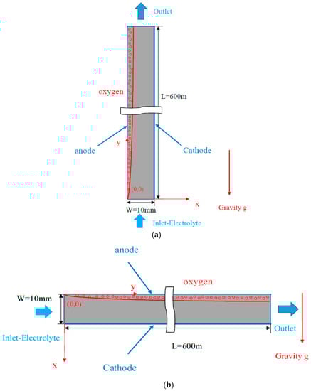
Figure 1.
Physical model: (a) A vertical electrolysis cell; (b) A horizontal electrolysis cell.

Table 1.
Physical properties of the gas phase flow at T = 25 °C.
2.1. Maxwell Equations for Electric Field
The applied voltage E (V) for given overall electric current flowing through the electrolysis cell can be decomposed:
where Ure is the reversible potential of chemical reaction, is the ohmic voltage drop in the biphasic electrolyte, R is the overall, and I is the current flowing through the cell, are the reaction overpotential and the concentration overpotential for anode and the cathode, respectively. The resistance of the electrolyte purpose of this paper is to investigate the effects of oxygen gas release at the anode on the void fraction, and the current density of a vertical and a horizontal electrolysis cell, respectively. Since it is difficult to solve such a problem with coupled equations and boundary conditions; expressing the kinetics of the electrochemical reaction at the electrodes, we assume that the reaction and concentration overpotentials at the electrodes are neglected.
With only the Ohmic component of resistance considered [9,10,13], Equation (1) can be reduced to:
The Gauss law may be written in the following form:
The electric field (V/m) can be defined by a unique electric potential scalar function U as follows:
Then, by plugging Equation (2) into Equation (1), the electric potential U is governed by the Laplace equations and is expressed as:
The current continuity equation is expressed by
where j (A/cm2) is the current density vector.
According to the Ohm’s law
where keff (S/m) is the effective electric conductivity of the electrolyte, which is a function of the local oxygen gas void fraction . Bruggemann’s relation [14] is used in the present study, where represents the electrical conductivity of the pure electrolyte (AN).
2.2. The Flow Field Equations for the Two-Phase Flow
A two-phase flow Eulerian–Eulerian method was used to analyze the oxygen production and the fluid distribution in an electrolysis cell. The model framework was based on the ensemble-averaged mass and momentum transport equations for each phase. By assuming that the mass exchange between two phases can be neglected, the continuity equation for the qth phase is:
where subscripts l and g refer to the liquid and gas phase, respectively, is void fraction of the fluid, and is defined as:
The momentum equation for the qth phase is
where g is the gravity force vector. The second term on the right-hand side of Equation (11) represents the body force. It should be noted that for a horizontal electrolysis cell, there is no buoyancy force to accelerate the movement of oxygen. The third term is an interaction force between the two phases, and the forth term corresponds to the momentum flux due to laminar and turbulent shear stresses, where its components are given by:
The total interfacial force acting between two phases may arise from several independent physical effects:
The forces indicated above respectively represent the interphase drag force , lift force , virtual mass force , the wall lubrication force , and the turbulence dispersion force [4]. The studies of Rampure et al. [15] and Diaz et al. [16] indicate that the inclusion of virtual mass force does not result in any significant difference in the dynamic and time-averaged flow properties. Therefore, in this present model, all forces except for the virtual mass force were considered.
The drag force is due to the resistance experienced by a body moving in the liquid.
where is the drag coefficient. The evaluation of the drag coefficient requires the bubble Reynolds number, which is based on the local slip velocity of a single bubble of constant diameter in the stagnant fluid. In the present computations, the drag coefficient was based on the Morsi and Alexander [17].
The lift force considered the interaction of the bubble with the shear field of the liquid. The lift force in terms of the slip velocity and the curl of the liquid phase velocity can be modeled as [18]:
where is the lift force coefficient. This lift force depends on the bubble diameter, the relative velocity between the phases, and the vorticity [19].
The turbulent dispersion force, derived by Lopez de Bertodano [20], is based on the analogy with molecular movement. The simplest way to model turbulent dispersion is to assume gradient transport as follows:
where is the liquid turbulent kinetic energy per unit of mass. The turbulent dispersion force has been using Bruns et al. model [21], and the turbulence dispersion coefficient of was recommended in the range of 0.1–1.0.
The wall lubrication force is because the liquid flow rate between the bubble and the wall is lower than between the bubble and the outer flow. The force is approximated as:
where is the relative velocity between phases. The is suggested by Antal et al. [22], , is the gas phase mean diameter, is the distance to the nearest wall, and the is the unit normal pointing away from the wall.
The standard turbulence model [23] embodied in the FLUENT 18.1 [24] CFD package was used. The transport equation for and are,
where the mixture density and velocity were calculated as,
The turbulent viscosity of the mixture, was computed from,
, denotes turbulent Prandtl number for kinetic energy and dissipation rate.
is the generation of turbulence kinetic energy in the mixture, based on gradients of mean velocity and turbulent viscosity, and it is computed from,
In the simulations, standard values of the model parameters [25] were used: ,, , , .
2.3. Boundary Conditions
Since the governing equations for the two-phase flow are elliptic, it is necessary to impose boundary conditions on all the boundaries in the computational domain. The upstream liquid inlet boundary condition is assumed to be uniform, where u0 = 0.4, 0.6, 1.0, and 1.5 m/s. At the downstream end of the computational domain, the streamwise gradient (Neumann condition) for the velocity is set to zero.
On the solid surfaces (anode and cathode), a no-slip boundary condition for the liquid velocity is applied, whilst for the gas phase, Sg is the release of mass flux for the oxygen (kg/m2 s) from the anode. For a case in which there is no back reaction (efficiency = 100%), Sg can be determined from Faraday’s law of electrolysis, Sg is
where n is the charge number, M is the molar weight of oxygen, F is the Faraday constant (96,485 C/mol). The accumulated oxygen mass flow rate :
The electrical potential difference between the anode and cathode was fixed at 5 V, which corresponded to a uniform current density j = 0.4 A/cm2 without any bubbles released from the electrodes.
3. Numerical Method
Since the oxygen-released mass flux Sg on the anode was coupled with the current density from Faraday’s Law, the electrical potential field (Equation (7)) and velocity field (Equations (8)–(23)) were coupled in the present study. The algorithm used to solve this coupling effect between the electric potential and velocity fields is shown in Figure 2. For the two-phase flow (the Eulerian–Eulerian model), the governing equations were solved numerically using the commercial software FLUENT 18.1 [17], whilst for the electrical potential field, a user-defined transport equation written in C language was incorporated in FLUENT 18.1.
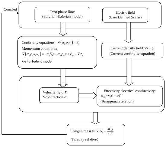
Figure 2.
The flow chart for the algorithm used to solve the coupling effect between the electric field and velocity field.
A grid system of 9000 (x = 30, y = 300) grid points is typically adopted in the computation domain, as shown in Figure 3. However, a careful check for the grid-independence of the numerical solutions was made to ensure the accuracy and validity of the numerical results. For this purpose, three grid systems, 15 × 300, 20 × 300, and 30 × 300, were used as tests. It was found that the relative errors for the local velocity and local void fraction between 20 × 300 and 30 × 300 were less than 1%. Computations are performed on a CPU E5-2650 v2 @ 2.60 GHz computer, and computation times were in the range of 4–6 h for each case. The convergence criterion was satisfied when the residuals of all variables were less than 1.0 × 10⁻⁶.
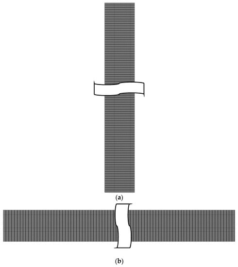
Figure 3.
Computational grid systems: (a) A vertical electrolysis cell; (b) A horizontal/vertical electrolysis cell.
4. Results and Discussion
Figure 4 shows the velocity distributions under four different inlet electrolyte (acrylonitrile, AN) velocities with vin = 0.4, 0.6, 1.0, and 1.5 m/s, at four different streamwise locations y (y = 50, 200, 400, and 600 mm), for a vertical and a horizontal electrolysis cell, respectively. It should be noted that the vertical Archimedes force on the bubble was only affected for the vertical electrolysis cell, but not for the horizontal cell. In addition, it was expected that the Archimedes force effect on the velocity distribution would be significant for a low inlet electrolyte velocity. This can be seen from Figure 4a–d for a vertical cell. When the inlet electrolyte velocity was 0.4 m/s, at y = 50 mm, the maximum velocity occurred at the cell center (x = 5 mm), while at y > 200 mm, the velocity near the anode was increased due to the Archimedes force on the oxygen bubble near the anode. It was observed that, for y = 600 mm, the maximum velocity no longer occurred at the center but rather occurred near the gas evolving electrode, and it was as high as 0.51 m/s. When the inlet electrolyte velocity reached 1.0 m/s and 1.5 m/s, this phenomenon almost disappeared, and the maximum velocities occurred at the cell center. On the contrary, this phenomenon hardly existed for the horizontal electrolysis cell. The velocity distributions for vin = 0.4, 0.6, 1.0, and 1.5 m/s were almost consistent with different inlet electrolyte velocities, and the maximum velocities were at the center, for which their corresponding numerical values were 0.466 m/s, 0.69 m/s, 1.138 m/s, and 1.69 m/s, respectively.
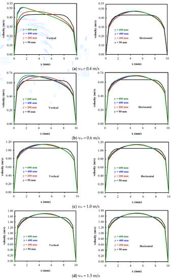
Figure 4.
The velocity distributions vs. x for different vin and y for a vertical cell and a horizontal cell.
Figure 5a,b show the void fraction contour under four different inlet electrolyte velocities, with vin = 0.4, 0.6, 1.0, and 1.5 m/s, for a vertical cell and a horizontal electrolysis cell, respectively. As expected, for a given velocity, the oxygen void fraction increased along with the streamwise direction (y). This was due to the accumulation of oxygen gas along with the electrode, and thus the total release of mass flow rate for oxygen was increased along with y. It was also seen that, for a given velocity, the void fraction for a horizontal cell was higher than for a vertical cell. In addition, as the velocity was increased, the void fraction decreased. The quantitative comparison is explained in the following paragraph.
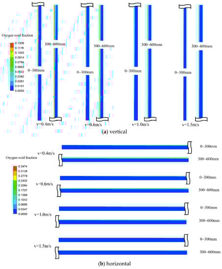
Figure 5.
The oxygen void fraction contour for different vin for a vertical cell and a horizontal cell.
Figure 6a–d illustrate the void fraction distributions α(x, y) vs. x (i.e., across the cell) under four different inlet electrolyte velocities, with vin = 0.4, 0.6, 1.0, and 1.5 m/s, respectively, at four different streamwise locations y (y = 100, 200, 400, and 600 mm), for a vertical cell and a horizontal electrolysis cell. The solid lines denote the results for a vertical cell, whilst the broken lines represent those from a horizontal cell. For a given velocity, the peak oxygen void fraction is shown to be increased along with y. For example, for vin = 0.4 m/s, the peak value increased from α = 0.06 at y = 100 mm to α = 0.131 at y = 600 mm for a vertical cell, whilst for a horizontal cell, the corresponding peak value increased from α = 0.11 to α = 0.347. It can also be observed that as the velocity was increased, the gas diffusion layer thickness decreased. This significantly decreased the void fraction. For example, at y = 600 mm, as the velocity increased from 0.4 to 1.5 m/s, the peak value decreased from α = 0.131 to α = 0.041 for a vertical cell, whilst for a horizontal cell, the corresponding peak value decreased from α = 0.347 to α = 0.062. One can also see that for a given velocity, the void fraction for a vertical cell is significantly lower than that for a horizontal cell.
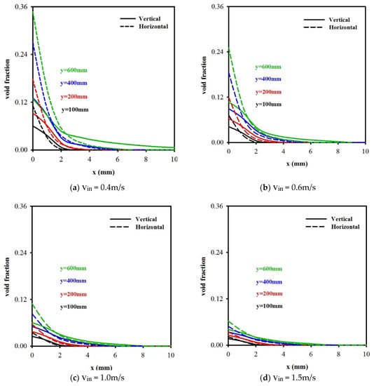
Figure 6.
The void fraction distribution vs. x for different vin and y for a vertical cell and a horizontal cell.
Figure 7a,b show the current density (j), the oxygen-released mass flux (Sg), and the total accumulated mass flow rate (), respectively, along the streamwise direction (y) of the electrode for a vertical cell and a horizontal cell with vin = 0.4 m/s. One can see that the increase in gas accumulation () resulted in a gradual decrease in current density (j), as well as a decrease in the oxygen-released mass flux (Sg) along the streamwise direction of the electrode. For example, for a vertical cell, when the electrode length was 300 mm and 600 mm, the corresponding current density jvertical, y=300mm = 0.3889 A/cm2 (decreased by 2.8%) and jvertical, y=600mm = 0.3796 A/cm2 (decreased by 5.1%), respectively, compared to that at the inlet (y = 0, j = 0.4 A/cm2), whilst for a horizontal cell, the decrease in the current density was higher, jhorizontal, y=300mm = 0.376 A/cm2 (decreased by 6.0%), and jhorizontal, y=600mm = 0.3596 A/cm2 (decreased by 10.1%), respectively. Additionally, showing for the comparison are the results (indicated in broken lines) for the case of uniform oxygen-released mass flux Sg, where Sg was calculated from Equation (8) by assuming the average current density j = 0.4 A/cm2. A close look at the figures indicates that the uniform oxygen-released mass flux Sg assumption for y = 600 mm overestimated the total gas accumulation mass flow rate () by 2.8% and 5.8% for a vertical cell and a horizontal cell, respectively, and underestimated the current density by 0.3% and 2.4% for a vertical cell and a horizontal cell, respectively.

Figure 7.
A comparison of current density and the release of mass flux for the oxygen and total accumulated mass flow rate along electrode y for coupled and de-coupled electric and velocity fields, with vin = 0.4 m/s.
Figure 8 illustrates the effects of three different inlet electrolyte velocities (vin = 0.6, 1.0, and 1.5 m/s) on the current density (j). The solid lines represent the results for a vertical cell, whilst the broken lines designate those for a horizontal cell. It was found that the current density increases with increases in the velocity. This is because as the velocity is increased, the void fraction decreases. For example, when the inlet velocity was 0.6 m/s, at y = 600 mm, for a vertical cell, the current density jvertical = 0.3850 A/cm2; when the velocity vin = 1.5 m/s, jvertical = 0.3934 A/cm2 (increased by 2.2%), whilst for a horizontal cell, there was a 5.2% increase when the velocity was increased from 0.6 to 1.5 m/s. It should be noted that as the velocity was increased, the difference in the current density between a vertical cell and a horizontal cell decreased. At y = 600 mm, for vin = 0.6 m/s, for a vertical cell, jvertical = 0.385 A/cm2, and jhorizontal = 0.3706 A/cm2, the difference was 3.9%; while for vin = 1.5 m/s, jvertical = 0.3934 A/cm2, and jhorizontal = 0.3921 A/cm2, the difference was only 0.33%.
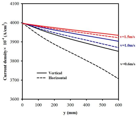
Figure 8.
A comparison of current density distribution along the electrode y for a vertical cell and a horizontal cell, with three different vin = 0.6, 1.0, and 1.5 m/s.
5. Conclusions
A two-phase Eulerian–Eulerian flow method was used to analyze the oxygen production and the fluid distribution in an electrolysis cell. Owing to the coupling between the oxygen-released mass flux (or void fraction), an iterative algorithm was developed to solve this coupling effect between the electric potential and velocity fields. For the two-phase flow, the governing equations were solved numerically using the commercial software FLUENT 18.1, whilst for the electrical potential field, a user-defined transport equation written in C language was incorporated in FLUENT 18.1. Based on the numerical results, the conclusions can be summarized as follows:
- The vertical Archimedes force on the bubble only existed for a vertical electrolysis cell, not for a horizontal cell, and this effect on the velocity distribution was significant only for a low inlet electrolyte velocity. For a lower velocity, the maximum velocity in the cell may no longer occur at the center but rather occurs near the gas evolving electrode, and this phenomenon disappears as the electrolyte velocity is increased.
- Given the accumulation of the oxygen gas along with the electrode, for a given velocity, the oxygen void fraction is increased along the streamwise direction. In addition, as the velocity is increased, the void fraction decreases. At y = 600 mm, as the velocity is increased from 0.4 to 1.5 m/s, the peak value is decreased from α = 0.131 to α = 0.041 for a vertical cell, whilst for a horizontal cell, the corresponding peak value is decreased from α = 0.347 to α = 0.062. The void fraction for a vertical cell is significantly lower than that for a horizontal cell.
- The uniform oxygen-released mass flux assumption will overestimate the total gas accumulation mass flow rate by 2.8% and 5.8% and underestimate the current density by 0.3% and 2.4%, for a vertical cell and a horizontal cell, respectively.
- The current density distribution was also affected by the inlet electrolyte velocity and the cell model (vertical or horizontal). As the velocity was increased from 0.6 m/s to 1.5 m/s, the current density at y = 600 mm was increased by 2.2% for a vertical cell, whilst for a horizontal cell, there was a 5.2% increase. As the velocity increases, the difference in the current density between a vertical cell and a horizontal cell decreases. This difference ranges from 3.9% to 0.33%, as the velocity is varied from 0.6 m/s to 1.5 m/s.
Author Contributions
All authors contributed to this work. J.-Y.J. performed the theoretical model.
Funding
This research was financially supported by the China Petrochemical Development Corporation, Taiwan.
Conflicts of Interest
The authors declare no conflict of interest.
Nomenclature
| drag coefficient | |
| lift force coefficient | |
| turbulence dispersion coefficient | |
| wall lubrication force coefficient | |
| dg | diameter of gas phase (m) |
| the electric field (V/m) | |
| E | applied voltage (V) |
| Ere | reversible potential (V) |
| F | Faraday constant (C/mol) |
| FD | drag force (N) |
| FL | lift drag (N) |
| Fgl | interfacial force (N) |
| FTD | turbulence dispersion force (N) |
| FVM | virtual mass force (N) |
| FWL | wall lubrication force (N) |
| g | gravity (m/s2) |
| the generation of turbulence kinetic energy in the mixture | |
| R | overall resistance of the electrolyte (Ω) |
| electric current density (A cm−2) | |
| k | turbulent kinetic energy |
| L | channel length (mm) |
| l | liquid |
| M | molar weight (kg/mol) |
| n | charge number |
| p | pressure (Pa) |
| Sg | gas phase source term- local oxygen mass flux (kg/m2 s) |
| oxygen accumulate mass flow rate (kg/s) | |
| u,v | velocity (m s−1) |
| U | electric potential (V) |
| Vq | the volume of the phase q |
| Vcell | the volume of the cell |
| W | width (mm) |
| x, y | Cartesian coordinates |
| Greek Symbols | |
| α | void fraction |
| transfer coefficient for anode and cathode | |
| ε | dissipation rate |
| the reaction overpotential and the concentration overpotential (V) | |
| turbulent Prandtl number for kinetic energy | |
| turbulent Prandtl number for dissipation rate | |
| κ0 | the electrical conductivity of the pure electrolyte (S/m) |
| κeff | effective electric conductivity of the electrolyte (S/m) |
| ρ | density of fluid (kg/m3) |
| μq | effective viscosity of phase q |
| τq | the stress tensor of the gas and liquid phase |
| Subscripts | |
| g,l | gas and liquid |
| p,q | fluid phase |
| i,j | x,y component |
| m | mixture |
References
- Karimi, F.; Mohammadi, F.; Ashrafizadef, S.N. An experimental study of the competing cathodic reactions in electrohydrodimerization of acrylonitrile. J. Electrochem. Soc. 2011, 158, 129–135. [Google Scholar] [CrossRef]
- Karimi, F.; Ashrafizadef, S.N.; Mohammadi, F. Process parameter impacts on adiponitrile current efficiency and cell voltage of an electromembrane reactor using emulsion-type catholyte. Chem. Eng. J. 2012, 183, 402–407. [Google Scholar] [CrossRef]
- Pfleger, D.; Gomes, S.; Gilbert, N.; Wagner, H.-G. Hydrodynamic simulations of laboratory scale bubble columns fundamental studies of the Eulerian-Eulerian modelling approach. Chem. Eng. Sci. 1999, 54, 5091–5099. [Google Scholar] [CrossRef]
- Ekambara, K.; Sanders, R.S.; Nandakumar, K.; Masliyah, J.H. CFD Simulation of bubbly two-phase flow in horizontal pipes. Chem. Eng. J. 2008, 144, 277–288. [Google Scholar] [CrossRef]
- Ali, B.A.; Pushpavanam, S. Analysis of unsteady gas–liquid flows in a rectangular tank: Comparison of Euler-Eulerian and Euler-Lagrangian simulations. Int. J. Multiph. Flow 2011, 37, 268–277. [Google Scholar]
- Tobias, C.W. Effect of Gas Evolution on current distribution and ohmic resistance in electrolyzers. J. Electrochem. Soc. 1959, 106, 833–838. [Google Scholar] [CrossRef]
- Dahlkild, A.A. Modelling the two-phase flow and current distribution along a vertical Gas-evolving Electrode. J. Fluid Mech. 2001, 428, 249–272. [Google Scholar] [CrossRef]
- Tsuge, H.; Tozawa, K.; Muguruma, Y.; Kawabe, M.; Abe, M.; Sagiyama, M. Effect of gas holdup on current density distribution in horizontal electrolysis cell. Can. J. Chem. Eng. 2003, 81, 707–712. [Google Scholar] [CrossRef]
- Nagai, N.; Takeuchi, M.; Nakao, M. Influences of bubbles between electrodes onto efficiency of alkaline water electrolysis. In Proceedings of the PSFVIP-4, Chamonix F 4008, Chamonix, France, 3–5 June 2003; pp. 1–10. [Google Scholar]
- Philippe, M.; Jérôme, H.; Sebastien, B.; Gérard, P. Modelling and calculation of the current density distribution evolution at vertical gas-evolving electrodes. Electrochim. Acta 2005, 51, 1140–1156. [Google Scholar] [CrossRef]
- Aldas, K.; Pehlivanoglu, N.; Mat, M.D. Numerical and experimental investigation of two-phase flow in an electrochemical cell. Int. J. Hydrog. Energy 2008, 33, 3668–3675. [Google Scholar] [CrossRef]
- Jupudi, R.S.; Zhang, H.; Zappi, G.; Bourgeois, R. Modeling bubble flow and current density distribution in an alkaline electrolysis cell. Int. J. Multiph. Flow 2009, 1, 341–347. [Google Scholar] [CrossRef]
- Kuhn, M.; Kreysa, G. Modelling of gas-evolving electrolysis cells. III. The iR drop at gas-evolving electrodes. J. Appl. Electrochem. 1989, 19, 720–728. [Google Scholar] [CrossRef]
- Bruggemann, D.A.G. Berechnung verschiedener physikalischer konstanten von heterogenen substnazen. Ann. Phys. 1935, 24, 636–664. [Google Scholar] [CrossRef]
- Rampure, M.R.; Buwa, V.V.; Ranade, V.V. Modelling of gas-liquid/gas-liquid-solid flows in bubble columns: Experiments and CFD simulations. Can. J. Chem. Eng. 2003, 81, 692–706. [Google Scholar] [CrossRef]
- Díaz, M.E.; Iranzo, A.; Cuadra, D.; Barbero, R.; Montes, F.J.; Galán, M.A. Numerical simulation of the gas–liquid flow in a laboratory scale bubble column Influence of bubble size distribution and non-drag forces. Chem. Eng. J. 2008, 139, 363–379. [Google Scholar] [CrossRef]
- Morsi, S.A.; Alexander, A.J. An Investigation of particle trajectories in two-phase flow systems. J. Fluid Mech. 1972, 55, 193–208. [Google Scholar] [CrossRef]
- Drew, D.A.; Lahey, R.T. Particulate Two-Phase Flow; Butterworth-Heinemann: Boston, MA, USA, 1993; pp. 509–566. [Google Scholar]
- Tomiyama, A. Struggle with computational bubble dynamics. In Proceedings of the Third International Conference on Multiphase Flow, Lyon, France, 8–12 June 1998. [Google Scholar]
- Lopez de Bertodano, M.; Lahey, R.T., Jr.; Jones, O.C. Turbulent bubbly two-phase flow in a triangular duct. Nucl. Eng. Des. 1994, 146, 43–52. [Google Scholar] [CrossRef]
- Burns, A.D.; Frank, T.; Hamill, I.; Shi, J.M. The favre averaged drag model for turbulent dispersion in Eulerian Multi-Phase flows. In Proceedings of the 5th International Conference on Multiphase Flow (ICMF’04), Yokohama, Japan, 30 May–4 June 2004; pp. 1–17. [Google Scholar]
- Antal, S.P.; Lahey, R.T.; Flaherty, J.E. Analysis of phase distribution in fully-developed laminar bubbly two phase flow. Int. J. Multiph. Flow 1991, 7, 635–652. [Google Scholar] [CrossRef]
- Elghobashi, S.E.; Abou-Arab, T.W. A two-equation turbulence model for two-phase flows. Phys. Fluids 1983, 26, 931–938. [Google Scholar] [CrossRef]
- Fluent Inc. ANSYS Fluent, Version, 18.1 User’s Guide; Fluent Inc.: New York, NY, USA, 2018. [Google Scholar]
- Launder, B.E.; Spalding, D.B. Lectures in Mathematical Models for Turbulence; Academic Press: London, UK, 1972. [Google Scholar]
© 2018 by the authors. Licensee MDPI, Basel, Switzerland. This article is an open access article distributed under the terms and conditions of the Creative Commons Attribution (CC BY) license (http://creativecommons.org/licenses/by/4.0/).