Fuzzy Byproduct Gas Scheduling in the Steel Plant Considering Uncertainty and Risk Analysis

Abstract

In the iron and steel enterprises, efficient utilization of byproduct gas is of great significance for energy conservation and emission reduction. This work presents a fuzzy optimal scheduling model for byproduct gas system. Compared with previous work, uncertainties in byproduct gas systems are taken into consideration. In our model, uncertain factors in byproduct systems are described by fuzzy variables and gasholder level constraints are formulated as fuzzy chance constraints. The economy and reliability of byproduct gas system scheduling are sensitive to different confidence levels. To provide a reference for operators to determine a proper confidence level, the risk cost is defined to quantify the risk of byproduct gas shortage and emission during the scheduling process. The best confidence level is determined through the trade-off between operation cost and risk cost. The experiment results demonstrated that the proposed method can reduce the risk and give a more reasonable optimal scheduling scheme compared with deterministic optimal scheduling.

1. Introduction

The iron and steel industry is an energy-intensive industry. According to statistics [1], it takes up more than 15% of China’s total energy demand. Therefore, efficient utilization of energy is very significant to cost saving in iron and steel enterprises. Byproduct gas is a kind of important secondary energy in the iron and steel industry. About 34% of coal is converted into byproduct gas during the production process [2,3]. Accordingly, the recovery and utilization of the byproduct gas are of great significance to achieving energy saving and emission reduction for iron and steel enterprises.

Byproduct gas is generated during the iron and steel making progress and is supplied to many related plants as a source of fuel. The remaining gas is sent to the self-provided power plant to generate steam and electricity. There is volatility in the generation and consumption of byproduct gas, and this would lead to an imbalance between gas supply and demand. An effective solution to this problem is to install gasholders as buffers. Since gasholders are limited in capacity, temporary excess and gas shortage usually occur. Therefore, it is necessary to optimize the scheduling of a byproduct gas system in advance to reduce byproduct gas shortage and flaring.

To make better use of byproduct gas, many researchers have devoted their work to the scheduling of byproduct gas in iron and steel enterprises. There are two typical scheduling methods, including the reasoning method [4,5] and the mathematical programming method [6,7,8,9,10,11,12,13,14]. The reasoning method formulates dispatching rules to maintain the gasholders within the safety operation zone. It has the advantages of simplicity and low computational time complexity. Compared with the reasoning method, the mathematical programming method can achieve an optimal solution. Akimoto et al. [6] first developed a mixed integer linear programming (MILP) model to optimize the gas scheduling by considering the stability of the byproduct gas system. Kim and Han [7] adopted the MILP model to optimize the gasholder level control and gas distribution on different boilers simultaneously. Integer variables ware adopted to express the switch states of the boiler burners. In 2010, Hong et al. [8] built the multiple period mathematical model according to the characteristics of the gas system. The model optimized the distribution of byproduct gas in both the cogeneration system and the production system. In 2013, Sun et al. [9,10] proposed a nonlinear mathematical programming model for byproduct gas scheduling by considering the change of boiler efficiency. And the decomposition and coordination method was developed to solve the optimization problem. In 2015, Zhao et al. [11,12] proposed the short period optimal scheduling model and discussed the influence of different weights on the results of optimal byproduct gas allocation. De Oliveira Junior et al. [13] improved the optimal scheduling model of byproduct gas system and proposed the rule-based weights determination method. In 2017, Hao et al. [14] established an MILP-based scheduling model to evaluate the load shifting potential of on-site power plant under time-of-use power price. MILP is an effective method to solve the optimal scheduling problem of byproduct gas. However, the models mentioned above assumed that there is no error in byproduct gas generation and consumption forecasting. In actual production processes, the amount of gas generation and consumption fluctuates greatly, and the inaccuracy of prediction would lead to uncertainties [15,16]. The optimal scheduling has the risk of violating constraints in some cases. Accordingly, it is of great significance to deal with the uncertainties correctly in the by-product gas scheduling to ensure the reliability of the gas system operation plan.

In this paper, we focus on byproduct gas system optimization scheduling considering prediction uncertainties. The generation and the consumption amount of byproduct gas are expressed as a fuzzy variable, and the fuzzy optimal scheduling model of the gas system is established. And the credibility theory is introduced to the model. The uncertainty constraints in the model are transformed into deterministic constraints to provide an efficient solution. Furthermore, the risk cost is defined to quantify the risk of byproduct gas shortage and emission during the scheduling process. The best confidence level is determined through the trade-off between operation cost and risk cost. Compared with existing work, the main contributions of this paper are as follows.

(1) We adopted the fuzzy optimal approach to byproduct gas scheduling to deal with uncertainties. To the authors’ knowledge, this is the first time that the fuzzy optimal approach has been used for this problem. And the fuzzy chance constrained programming is introduced to coordinate profit and risk.

(2) To evaluate the risk caused by uncertainties, including byproduct gas shortage and emission, the risk cost is defined in this paper. Furthermore, the risk cost is used to help dispatchers select the appropriate confidence level.

The rest of the paper is organized as follows. Fuzzy chance constrained programming and credibility distribution of fuzzy variables are introduced in Section 2. The overall byproduct gas system is described in Section 3, and the influence of uncertainty on byproduct gas system is analyzed. Section 4 demonstrates mathematical formulation on fuzzy byproduct gas scheduling. Risk analysis of byproduct gas system scheduling is provided in Section 5. Section 6 presents the results from a case study. Finally, the paper is concluded in Section 7.

2. Fundamentals

2.1. Fuzzy Chance Constrained Programming

The optimization problem containing fuzzy variables in constraint conditions can be expressed as follows.

$$\begin{array}{c}\min f(x)\\ s.t.\hspace{1em}{g}_j(x,\xi )\le 0,j=1,2,\dots n\end{array}$$

(1)

where $x$ is the decision vector, $f(x)$ is the objective function, and $g_j(x,\xi )$ is the constraint function. As there are fuzzy variables in constraints, it is difficult to provide a certainly feasible solution. Therefore, credibility theory is introduced to solve this problem. The constraints containing fuzzy variables are satisfied with the pre-given confidence level.

$$C_r\{g_j(x,\xi )\le 0\}\ge \alpha$$

(2)

In Equation (2), $\alpha$ is the confidence level, $C_r\{\}$ is the credibility measure of the constraints.

2.2. Crisp Equivalents

The key to solve the fuzzy chance constrained optimization problem is to deal with constraints containing fuzzy variables. Reference [17] provides a method which transforms chance constraints containing multiple fuzzy parameters to crisp equivalents, so that the problem can be solved by traditional methods. Assume that the function $g_j(x,\xi )$ is written as follows:

$$g_j(x,\xi )=h_1(x){\xi }_1+h{(x)}_2{\xi }_2+\dots +h{(x)}_m{\xi }_m+h_0(x)$$

(3)

${\xi }_k$ is the triangle variable ($r_{k1}$, $r_{k2}$, $r_{k3}$), $k=1,2,\dots ,m$. The confidence level $\alpha$ is commonly set to a value higher than 0.5 in fuzzy chance constrained programming. For $\alpha \ge 0.5$, we have $C_r\{g(x,\xi )\le 0\}\ge \alpha$, if and only if

$$h_0(x)+(2\alpha -1){\displaystyle \sum _{k=1}^m[r_{k3}{h}_k^{+}(x)-r_{k1}{h}_k^{-}(x)]}\le 0$$

(4)

here,

$$h_k^{+}(x)=\{\begin{array}{ll}{h}_k(x),& \mathrm{if}{h}_k(x)\ge 0\\ 0,& \mathrm{if}{h}_k(x)<0\end{array}$$

(5)

$$h_k^{-}(x)=\{\begin{array}{ll}0,& \mathrm{if}{h}_k(x)\ge 0\\ -h_k(x),& \mathrm{if}{h}_k(x)<0\end{array}$$

(6)

2.3. Credibility Distribution of Fuzzy Variables

According to reference [18], $\xi$ is assumed to be a fuzzy variable. If function $\mathsf{\Phi }:[-\infty ,+\infty ]\to$ [0, 1] satisfies

$$\mathsf{\Phi }(x)=Cr\{\theta \in \mathsf{\Theta }|\xi (\theta )\le x\},$$

(7)

then $\mathsf{\Phi }$ is defined as the credibility distribution of $\xi$.

If function $\varphi :R\to [0,+\infty ]$ for $x\in [-\infty ,+\infty ]$ satisfies

$$\mathsf{\Phi }(x)={\displaystyle {\int }_{-\infty }^x\varphi (y)dy},$$

(8)

then $\varphi$ is defined as dependability density function of $\xi$.

Assume that $\xi$ is a triangle fuzzy variable ($r_1$, $r_2$, $r_3$), the credibility distribution function of $\xi$ is

$$\mathsf{\Phi }(x)=\{\begin{array}{cc}0,& \mathrm{if}x\le r_1\hfill \\ \frac{x-r_1}{2(r_2-r_1)},& \mathrm{if}{r}_1\le x\le r_2\hfill \\ \frac{x+r_3-2r_2}{2(r_3-r_2)},& \mathrm{if}{r}_2\le x\le r_3\hfill \\ 1,& \mathrm{if}{r}_3\le x\hfill \end{array}$$

(9)

The credibility density function of $\xi$ is

$$\varphi (x)=\{\begin{array}{cc}\frac{1}{2(r_2-r_1)},& \mathrm{if}{r}_1\le x\le r_2\hfill \\ \frac{1}{2(r_3-r_2)},& \mathrm{if}{r}_1\le x\le r_2\hfill \\ 0,& \mathrm{otherwise}\hfill \end{array}$$

(10)

3. Problem Description

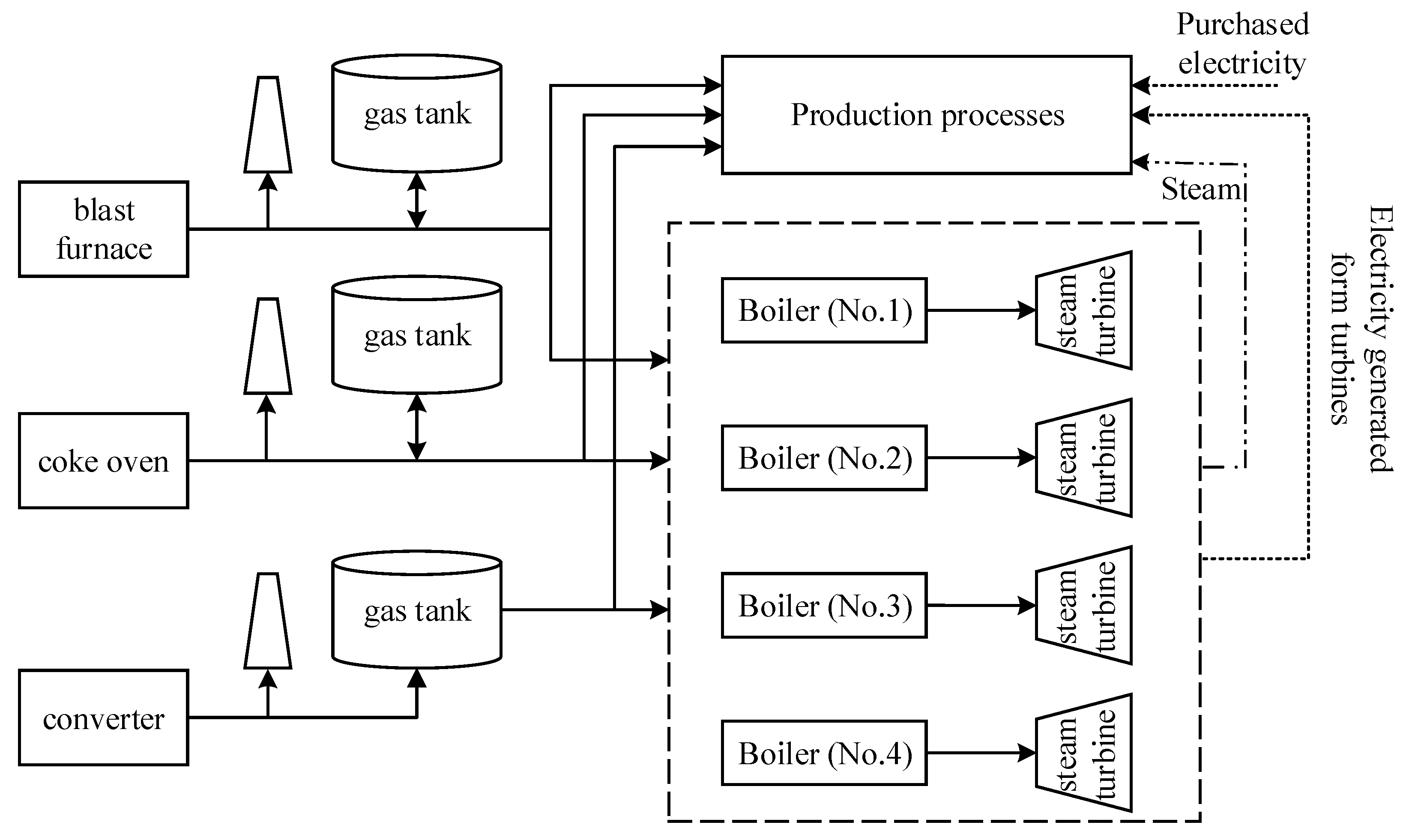
As shown in Figure 1, byproduct gas generated in iron and steel plant includes blast furnace gas (BFG), coke oven gas (COG), and Linz-Donawitz converters gas (LDG). After the byproduct gas is produced, it is transported to various production units through the gas pipe network to provide the necessary energy. The remaining gas is sent to the gas boiler of the self-owned power plant to generate electricity through a steam turbine. The gasholder is a storage device in the gas system, which plays a role of buffer. Byproduct gas is first supplied to production equipment. And the gas consumption of production equipment cannot be controlled by the operators of the byproduct distribution system. Then the surplus gas is consumed by boilers in the power plant. The power plant consumption can be controlled following the scheduling plan.

The optimization problem of byproduct gas distribution is to find a solution that maintains the stability of the byproduct gas system and minimizes the electricity purchasing. The stability of the byproduct gas system includes the gasholder stability and the boiler operation stability. The amount of gas in the gasholder is expected to be maintained near the normal level to avoid gas shortage and emission. The stability of boilers is achieved by minimize the switching times of the burners. In recent years, some studies have been performed on optimal distribution of byproduct gas.

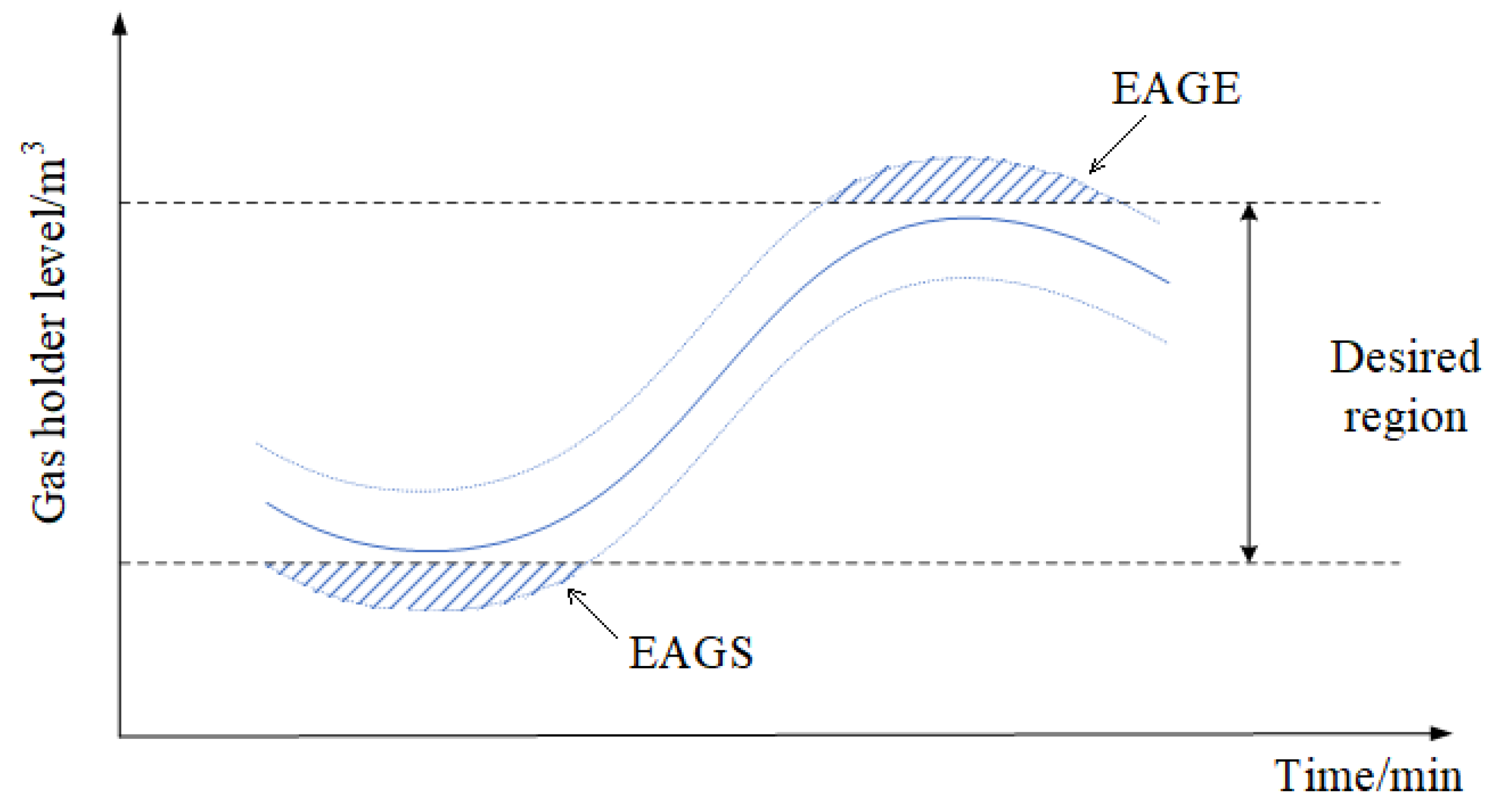
The models of byproduct gas system scheduling are mainly based upon the forecasting of gas generation and consumption. Since the gas generation and consumption fluctuate greatly, the prediction error of the gas generation and consumption is inevitable. Therefore, the scheduling process is faced with many uncertainties. As shown in Figure 2, if the predicted value is completely accurate, the gas holder could be maintained within the safe region. For example, affected by the uncertainties of gas generation and consumption, the holder level may be lower than the minimum safe level (named expected additional gas shortage, EAGS) or upper than the maximum safe level (named expected additional gas excess, EAGE), which leads to the risk of byproduct gas shortage or emission. A simple way to solve this problem is to reserve part of gas holder volume. Nevertheless, the reserved volume reduces the adjustable volume of the gas holder, resulting in an increase of the system operation cost. Therefore, to deal with the uncertainties, the risk of byproduct gas shortage or emission should be controlled within a certain range, and the benefit and the risk are expected to be balanced.

4. Model Establishment for Byproduct Gas Scheduling

4.1. Fuzzy Variables in Byproduct Gas System

One of the main characters of the fuzzy approach is that uncertain parameters can be expressed by fuzzy variables. In our work, triangle membership function is applied to express the generation and consumption of byproduct gas. The maximum, minimum, and the most possible values of the generation and consumption of byproduct gas can be obtained by forecasting tools [19,20,21,22]. Fuzzy parameters of the byproduct gas generation and consumption can be stated as follows.

$$Q_{gen,F,t}^G=({\underset{\_}{Q}}_{gen,t}^G,Q_{gen,t}^G,{\overline{Q}}_{gen,t}^G)=Q_{gen,t}^G(r_{gen,1}^G,r_{gen,2}^G,r_{gen,3}^G),\forall t$$

(11)

$$Q_{con,F,t}^G=({\underset{\_}{Q}}_{con,t}^G,Q_{con,t}^G,{\overline{Q}}_{con,t}^G)=Q_{con,t}^G(r_{con,1}^G,r_{con,2}^G,r_{con,3}^G),\forall t$$

(12)

In the upper equations, $Q_{gen,F,t}^G$ and $Q_{con,F,t}^G$ are fuzzy parameters of byproduct gas generation and consumption at time t, $Q_{gen,t}^G$ and $Q_{con,t}^G$ are the predicted values of byproduct gas generation and consumption at time t. ${\overline{Q}}_{gen,t}^G$ and ${\overline{Q}}_{con,t}^G$ are the upper bounds, ${\underset{\_}{Q}}_{gen,t}^G$ and ${\underset{\_}{Q}}_{con,t}^G$ are the lower bounds. $r_{gen,1}^G$ − $r_{gen,3}^G$ and $r_{gen,1}^G$ − $r_{gen,3}^G$ correspond to the scaling factors of byproduct gas generation and consumption respectively.

4.2. Objective Function

According to the analysis of Section 3, the formulated objective function aims to minimize the operation cost of the byproduct gas system. The operation cost includes the gasholder penalty cost, the burner switching cost, and the electricity purchasing cost. Accordingly, the operation cost is expressed as follows.

$$\min {\displaystyle \sum _{t=1}^T\left\{\left({\displaystyle \sum _G{W}_{dev}^G\Delta V_{dev,t}^G+{\displaystyle \sum _G{W}_{flar}^G{V}_{flar,t}^G}}\right)+{\displaystyle \sum _G{\displaystyle \sum _{i=1}^{N_B}{W}_{sw}^G\Delta N_{i,t}^G+C_{elec}(E_{dem,t}-E_{gen,t})}}\right\}}$$

(13)

In Equation (13), the first term denotes the gasholder deviation cost and byproduct gas flaring cost. $\Delta V_{dev,t}^G=\left|V_t^G-V_{nor,t}^G\right|$ shows the difference between the current gasholder level and the normal gasholder level. $V_{flar,t}^G$ indicates the amount of byproduct gas emission. The second term denotes the burner switching cost. $\Delta N_{i,t}^G=\left|n_{i,t}^G-n_{i,t-1}^G\right|$ is the number of burner switches of boilers. The third part states purchased electricity cost. $E_{dem,t}$ is the demand for electricity and $E_{gen,t}$ denotes the amount of electricity generated by power plants. $C_{elec}$ is the unit cost of electricity.

4.3. Constraints

4.3.1. Constraints of Gas Holders

The mass balance constraint of gas holders is as follows:

$$V_t^G-V_{t-1}^G=Q_{gen,t}^G-Q_{con,t}^G-{\displaystyle \sum _{i=1}^{N_B}{Q}_{i,t}^G}-Q_{flar,t}^G$$

(14)

$V_t^G$ is the gasholder level at time t and $V_{t-1}^G$ is the gasholder level at time t − 1. The difference of the gasholder level between the two periods $V_t^G-V_{t-1}^G$ equals to the surplus amount of the byproduct gas (the generation $Q_{gen,t}^G$ minus the consumption $Q_{con,t}^G$) minus the sum of the gas consumption in boilers $Q_{i,t}^G$, and then minus the gas emission amount, $Q_{flar,t}^G$.

To prevent operational risks in the gasholder, it is necessary to restrict the safety range of the gasholder. Equations (15) and (16) represents the safety constraints.

$$V_{t-1}^G+Q_{gen,t}^G-Q_{con,t}^G-{\displaystyle \sum _{i=1}^{N_B}{Q}_{i,t}^G}-Q_{flar,t}^G\ge V_L^G$$

(15)

$$V_{t-1}^G+Q_{gen,t}^G-Q_{con,t}^G-{\displaystyle \sum _{i=1}^{N_B}{Q}_{i,t}^G}-Q_{flar,t}^G\le V_H^G$$

(16)

$V_L^G$ represents the minimum safe level of the gasholder, and $V_H^G$ represents the maximum safe level of the gasholder in Equation (16).

In deterministic models, the amount of gas production and consumption are expressed by predicted values, and the predicted values are assumed to be error-free in Equations (15) and (16). However, the scheduling results may have the risk of violating the safety constraints if prediction errors are not considered. In our work, the uncertainty of gas generation and consumption predictions are considered, and fuzzy variables are used to express the generation and consumption of byproduct gas. The credibility chance constraint of the gasholder can be expressed as follows:

$$Cr\left\{V_{t-1}^G+Q_{gen,F,t}^G-Q_{con,F,t}^G-{\displaystyle \sum _{i=1}^{N_B}{Q}_{i,t}^G}-Q_{flar,t}^G\ge V_L^G\right\}\ge \alpha$$

(17)

$$Cr\left\{V_{t-1}^G+Q_{gen,F,t}^G-Q_{con,F,t}^G-{\displaystyle \sum _{i=1}^{N_B}{Q}_{i,t}^G}-Q_{flar,t}^G\le V_U^G\right\}\ge \alpha$$

(18)

The confidence level α is used to characterize the credibility of constraint satisfaction. The confidence level reflects the decision maker’s expectation of constraint satisfaction. According to Section 2.2, Equations (17) and (18) can be converted to the following crisp equivalents.

$$V_{t-1}^G+Q_{gen,t}^G-Q_{con,t}^G+(2\alpha -1)({\underset{\_}{Q}}_{gen,t}^G-{\overline{Q}}_{con,t}^G)-{\displaystyle \sum _{i=1}^{N_B}{Q}_{i,t}^G}-Q_{flar,t}^G\ge V_L^G$$

(19)

$$V_{t-1}^G+Q_{gen,t}^G-Q_{con,t}^G+(2\alpha -1)({\overline{Q}}_{gen,t}^G-{\underset{\_}{Q}}_{con,t}^G)-{\displaystyle \sum _{i=1}^{N_B}{Q}_{i,t}^G}-Q_{flar,t}^G\le V_H^G$$

(20)

4.3.2. Constraints of Boilers and Turbines

The surplus byproduct gas is used as fuel of the boilers. The energy and mass balance constraints of boilers are as follows.

$${\displaystyle \sum _G{H}^G{Q}_{i,t}^G=\frac{H^{stm}{Q}_{i,t}^{stm}-H^{wat}{Q}_{i,t}^{wat}}{{\eta }_i^b}}$$

(21)

$$Q_{i,t}^{stm}=Q_{i,t}^{wat}$$

(22)

$$Q_{i,t}^G=M_i^G{n}_{i,t}^G$$

(23)

Equation (21) represents the energy balance of boilers. The amount of thermal energy generated by byproduct gas burning in a boiler ${\displaystyle \sum _G{H}^G{Q}_{i,t}^G}$ is equal to the value of energy used to heat the water into steam. Due to the energy losses in the process, the efficiency of the boiler ${\eta }_i^b$ is taken into account. $Q_{i,t}^{stm}$ indicates the amount of steam generated by the boiler, $Q_{i,t}^{wat}$ is the amount of water in the boiler. Equation (23) states that the amount of byproduct gas consumed by the boiler $Q_{i,t}^G$ equals to the gas consumption volume in each burner $M_i^G$ multiplied by the number of the open burners in period t.

In the power plant, steam is used to generate electricity through the turbines. The energy and mass balance in the power generation process can be expressed as follows.

$$p{w}_{gen,j,t}=Q_{j,t}^{tb}{H}^{stm}{\eta }_j^{tb}$$

(24)

$$E_{gen,t}={\displaystyle \sum _{j=1}^{N_T}p{w}_{gen,j,t}}$$

(25)

$$Q_{i,t}^{stm}=Q_{i,t}^{dem}+Q_{i,t}^{tb}$$

(26)

In Equation (24), the electricity generated by the steam turbine $p{w}_{gen,j,t}$ is equal to the amount of steam into the turbine $Q_{j,t}^{tb}$ multiplied by enthalpy of steam $H^{stm}$ and the efficiency of the turbine ${\eta }_j^{tb}$. Steam balance is expressed by Equation (26). $Q_{i,t}^{dem}$ represents the demand for steam in the production process.

According to Equations (13), (14), (19)–(26), the by-product gas optimization scheduling model is established based on fuzzy chance constrained optimization.

5. Risk Analysis of Byproduct Gas System Scheduling

Although the constraints are satisfied with a certain confidence level, there still exists the risk of gas shortage or excess during byproduct gas dispatching. In this section, the risk of gas shortage and excess is quantified, and then the risk cost is defined. Furthermore, the appropriate confidence level is selected by making a compromise between the operating cost and risk cost of the system.

According to Equation (14), the gas holder level can be expressed as follows.

$$V_t^G=V_{t-1}^G+Q_{gen,t}^G-Q_{con,t}^G-{\displaystyle \sum _{i=1}^{N_B}{Q}_{i,t}^G}-Q_{flar,t}^G$$

(27)

According to additional rules of the fuzzy variables, the gasholder level is a triangle fuzzy variable $V_{F,t}^G$ expressed as $({\underset{\_}{V}}_t^G,V_t^G,{\overline{V}}_t^G)$, here

$$\{\begin{array}{l}{\underset{\_}{V}}_t^G=V_{t-1}^G+{\underset{\_}{Q}}_{gen,t}^G-{\overline{Q}}_{con,t}^G-{\displaystyle \sum _{i=1}^{N_B}{Q}_{i,t}^G}-Q_{flar,t}^G\\ V_t^G=V_{t-1}^G+Q_{gen,t}^G-Q_{con,t}^G-{\displaystyle \sum _{i=1}^{N_B}{Q}_{i,t}^G}-Q_{flar,t}^G\\ {\overline{V}}_t^G=V_{t-1}^G+{\overline{Q}}_{gen,t}^G-{\underset{\_}{Q}}_{con,t}^G-{\displaystyle \sum _{i=1}^{N_B}{Q}_{i,t}^G}-Q_{flar,t}^G\end{array}$$

(28)

According to Section 2.3, the credibility density function of $V_{F,t}^G$ is

$${\varphi }_s(x)=\{\begin{array}{cc}\frac{1}{2(V_t^G-{\underset{\_}{V}}_t^G)},& \mathrm{if}{\underset{\_}{V}}_t^G\le x\le V_t^G\hfill \\ \frac{1}{2({\overline{V}}_t^G-V_t^G)},& \mathrm{if}{V}_t^G\le x\le {\overline{V}}_t^G\hfill \\ 0,& \mathrm{otherwise}\hfill \end{array}$$

(29)

The risk of byproduct gas scheduling mainly includes the risk of EAGS and the risk of EAGE, which can be seen in the Section 3, Figure 2. The risks of EAGS and EAGE as follows:

$$R_{EAGS}^G=\{\begin{array}{ll}{\displaystyle \sum _{t=1}^T}{\displaystyle {\int }_{{\underset{\_}{V}}_t^G}^{V_L^G}}(V_L^G-x){\varphi }_s(x)dx,& \mathrm{if}{\underset{\_}{V}}_t^G\le V_L^G\hfill \\ 0,& \mathrm{otherwise}\hfill \end{array}$$

(30)

$$R_{EAGE}^G=\{\begin{array}{ll}{\displaystyle \sum _{t=1}^T}{\displaystyle {\int }_{V_H^G}^{{\overline{V}}_t^G}}(x-V_H^G){\varphi }_s(x)dx,& \mathrm{if}{\overline{V}}_t^G\ge V_H^G\hfill \\ 0,& \mathrm{otherwise}\hfill \end{array}$$

(31)

Accordingly, the risk cost (RC) of byproduct gas system is defined as

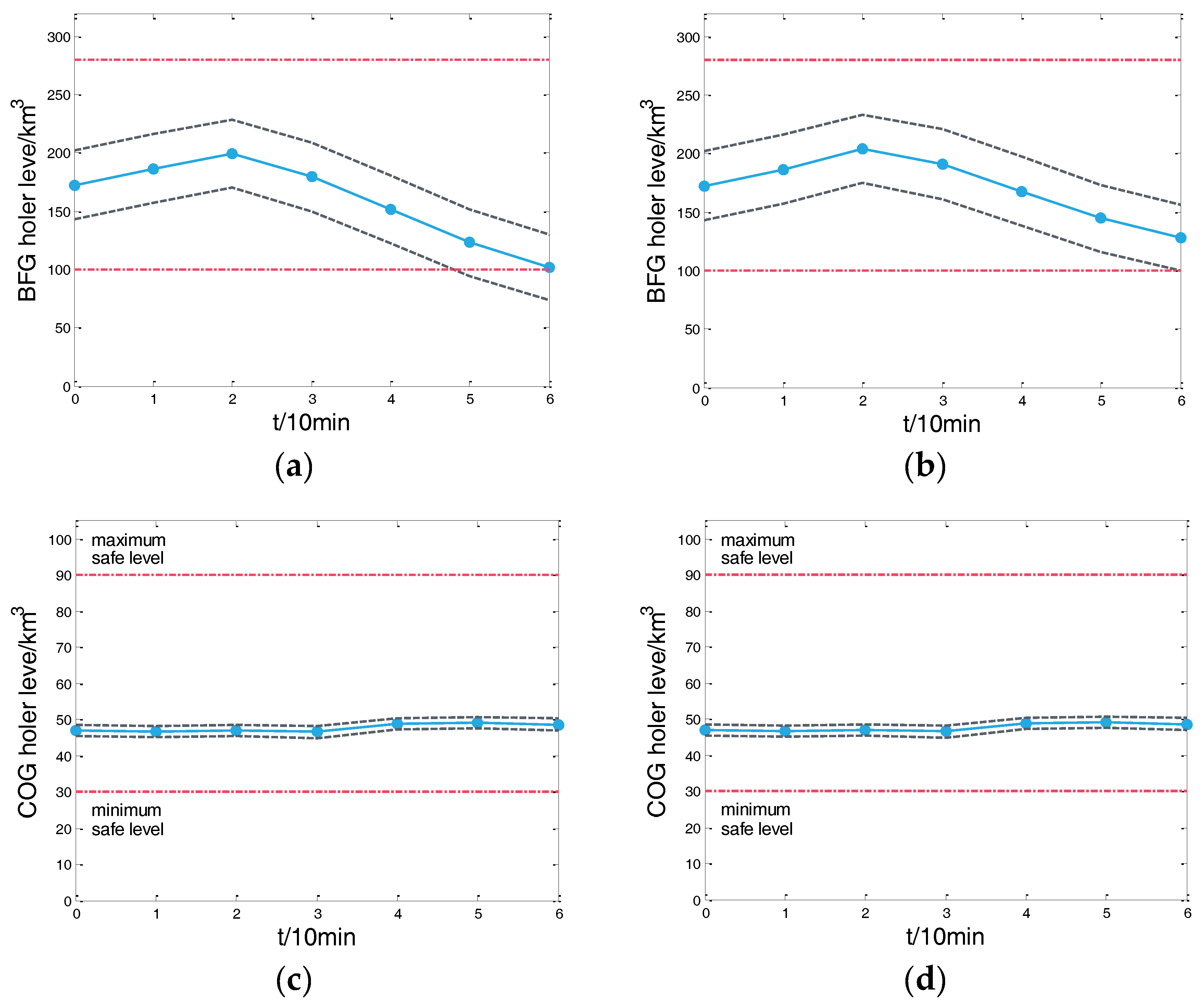
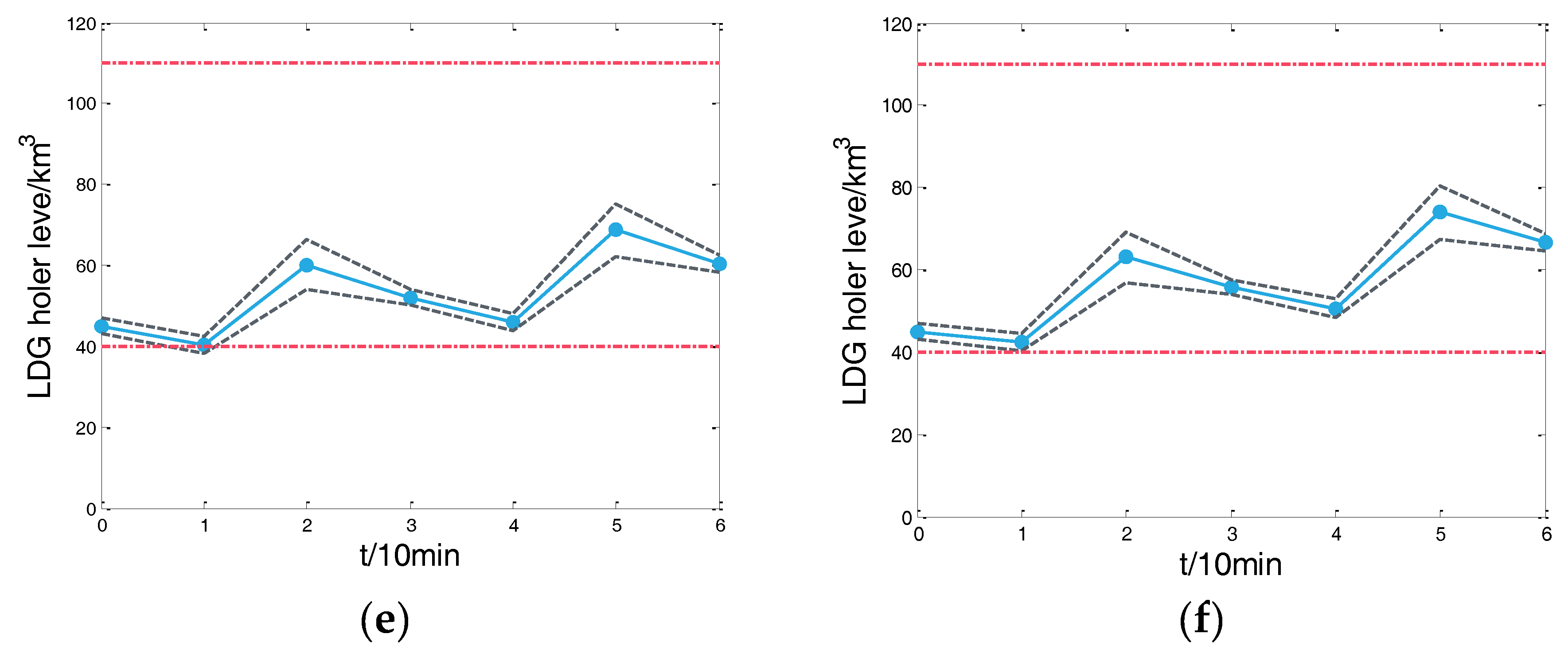
$$RC={\displaystyle \sum _G{\lambda }_1^G{R}_{EAGS}^G+{\lambda }_2^G{R}_{EAGE}^G}$$

(32)

${\lambda }_1^G$ and ${\lambda }_2^G$ represent the risk coefficients, which can be determined by actual situations. In our work, ${\lambda }_1^G$ and ${\lambda }_2^G$ were set to $50\times W_{dev}^G$ and $25\times W_{dev}^G$ respectively. The meaning of the variables mentioned above can be seen in the Nomenclature.

6. Case Study

6.1. Parameters of the Test System

To verify the proposed method, a case study was conducted for a steel plant. There were eight blast furnaces, six coke ovens, six converters, and three gas holders in this plant. Parameters of the gasholders are shown in

Table 1. Maximum safe level, normal level, and minimum safe level (m³) of gasholders.

	Maximum Safe Level	Normal Level	Minimum Safe Level
BFG	280,000	150,000	100,000
COG	90,000	50,000	30,000
LDG	110,000	60,000	40,000

. The on-site power plant contained four 220 t/h boilers and four 50 MW steam turbines. The efficiency of the boilers and turbines are listed in

Table 2. Parameters of boilers.

	1#Boiler	2#Boiler	3#Boiler	4#Boiler
Efficiency	0.87	0.85	0.82	0.85

and

Table 3. Parameters of turbines.

	1#TB	2#TB	3#TB	4#TB
Efficiency	0.26	0.25	0.24	0.26

, respectively. Each boiler could burn all three kinds of gas and there were 12 burners for each kind of gas. The maximum consumptions of BFG, COG, and LDG for each boiler were 1.2 × 10⁵ m³h⁻¹, 1.2 × 10⁴ m³h⁻¹ and 3 × 10⁴ m³h⁻¹ respectively. The time duration of this study was 1h, and it was divided into six periods with a 10 min each period. This was suitable for byproduct gas system dispatching. The predicted values of byproduct gas generation and consumption in each period are shown in

Table 4. Gas generation and consumption volumes (m³) in each period.

Period	BFG		COG		LDG
	Generation	Consumption	Generation	Consumption	Generation	Consumption
1	420,870	336,870	31,512	25,212	12,260	4392
2	415,246	332,646	32,242	25,342	39,258	4887
3	403,055	356,149	33,001	26,601	11,432	4149
4	387,614	350,708	31,742	22,942	13,069	3604
5	382,064	345,158	32,395	25,295	42,029	4029
6	375,858	332,395	32,042	25,942	12,488	5232

and their triangle fuzzy scaling factors are listed in

Table 5. Triangle fuzzy scaling factors of gas generation and consumption.

Fuzzy Variable		r1	r2	r3
BFG	generation	0.97	1	1.03
	consumption	0.95	1	1.05
COG	generation	0.99	1	1.01
	consumption	0.95	1	1.05
LDG	generation	0.85	1	1.15
	consumption	0.95	1	1.05

.

6.2. Comparison of Fuzzy Scheduling and Deterministic Scheduling

To verify the performance of the fuzzy optimization model of the byproduct gas system, the proposed method is compared with the deterministic scheduling. In the experiments, the confidence level of fuzzy chance constraints is set to 1. A comparison of the gasholder level between deterministic scheduling and fuzzy scheduling results is shown in Figure 3. The BFG, COG, and LDG holder levels obtained by deterministic scheduling are illustrated in Figure 3a,c,e. And the BFG, COG, and LDG holder levels obtained by fuzzy scheduling are shown in Figure 3b,d,f. In each subfigure of Figure 3, the solid curves represent the gasholder level trend and the dashed curves represent the upper and lower bound of the gasholder level trend.

According to the fuzzy optimal scheduling, the gasholder levels are running within the safety region in all time periods and there exists no risk of gas shortage or emission, which can be seen in Figure 3b,d,f. Comparatively, for the scheduling results obtained by the deterministic model, the lower bound of the LDG holder level in the first period and the lower bound of the BFG holder level in the fifth and the sixth period are lower than the minimum safety gasholder levels, as shown in Figure 3a,e. This leads to the risk of byproduct gas shortage. That is because the effect of prediction uncertainties was not considered in the deterministic model. There was not enough gasholder capacity reserved for the uncertainty. The experiment proved that the proposed method can improve the reliability of the byproduct system.

The optimal scheduling operation costs obtained by the two models are shown in

Table 6. Comparison of cost (US$) based on two models.

	Purchasing Electricity Cost	Gasholder Level Deviation Cost	Burner Switching Cost	Operation Cost	Risk Cost
Deterministic Model	4333	2162	1427	7922	2553
Fuzzy Model	5135	1975	2140	9250	0

. The operational cost obtained by the fuzzy optimization scheduling is higher than the operational cost obtained by the deterministic optimal scheduling. This is because, to reduce the risk of gas shortage and emission, more reserve capacity of gasholder is needed. Therefore, burner switching of the boiler increases and electricity generation relatively reduces. To a certain extent, the operation cost increases.

6.3. Analysis on Confidence Levels

In this section, an analysis is carried out to verify the impact of confidence levels on system scheduling. The initial and final values of the confidence level were set to 0.65 and 1.0, and the step size was 0.05. The operation costs and the risk cost at different confidence levels are shown in

Table 7. Fuzzy optimal scheduling results under different confidence levels.

Confidence Level	Operation Cost (US$)	Risk Cost (US$)	Total Cost (US$)
0.65	8054	1166	9220
0.70	8204	749	8953
0.75	8212	599	8811
0.80	8478	315	8793
0.85	8695	220	8915
0.90	8928	25	8953
0.95	8933	21	8954
1.00	9250	0	9250

. It can be seen from Table 7 that with the increase of the confidence levels, the risk cost decreases while the operation cost increases. The results indicated that the improvement of system reliability is at the expense of increasing system operation cost. Therefore, selecting an appropriate confidence level is indispensable to make a reasonable compromise between the economy and the risk of the byproduct gas system.

The total cost, which is the sum of the risk cost and the operation cost, was calculated. The results show that the lowest total cost is achieved at the confidence level of 0.8. Thus, 0.8 is the appropriate confidence level. It is noteworthy that because the confidence level changes with 0.05, appropriate confidence level is roughly estimated. To get a more accurate value, further subdivision of confidence level is needed.

7. Conclusions

The optimal scheduling of byproduct gas systems in iron and steel enterprises faces many uncertain factors, such as gas generation and consumption fluctuations. To deal with the uncertainty of gas system scheduling, a fuzzy optimization scheduling model for byproduct gas system is established based on fuzzy chance constrained programming method. Byproduct gas generation and consumption are described as fuzzy variables. To obtain the optimal confidence level, risk cost is introduced, which qualify the risk of the scheduling results under different confidence levels. The production data of a steel enterprise is used to evaluate the proposed method. Experimental results showed the proposed method can improve the reliability of the byproduct gas scheduling compared with the deterministic method. At the same time, the risk cost can help dispatchers determine an optimal confidence level to reduce system operation cost while maintaining system reliability.

References

1. National Bureau of Statistics of China. Consumption of Electricity and Its Main Varieties by Sector. Available online: http://data.stats.gov.cn/english/easyquery.htm?cn=C01 (accessed on 9 June 2018).
2. Li, X.; Zhang, C.; Huang, D. Interpretation and implementation suggestions for norm of energy consumption per unit product of major individual process of GB 21256—2013 crude steel manufactory process. China Metall. 2016, 26, 47–61. [Google Scholar]
3. Bernhart, S.; Frank, H.; Olaf, H. Realized measures for energy efficient process gas use in metallurgical plants. World Steel 2012, 12, 60. [Google Scholar]
4. Zhao, J.; Wang, W.; Liu, Y.; Pedrycz, W. A two-stage online prediction method for a blast furnace gas system and its application. IEEE Trans. Control Syst. Technol. 2011, 19, 507–520. [Google Scholar] [CrossRef]
5. Li, H.; Wang, J.; Wang, H.; Meng, H. An optimal method for prediction and adjustment on gasholder level and self-provided power plant gas supply in steel works. J. Central South Univ. 2014, 21, 2779–2792. [Google Scholar] [CrossRef]
6. Akimoto, K.; Sannomiya, N.; Nishikawa, Y.; Tsuda, T. An optimal gas supply for a power plant using a mixed integer programming model. Automatica 1991, 27, 513–518. [Google Scholar] [CrossRef]
7. Kim, J.H.; Yi, H.S.; Han, C. A novel MILP model for plantwide multiperiod optimization of byproduct gas supply system in the iron-and steel-making process. Chem. Eng. Res. Des. 2003, 81, 1015–1025. [Google Scholar] [CrossRef]
8. Kong, H.; Qi, E.; Li, H. A MILP model for optimization of byproduct gases in the integrated iron and steel plant. Appl. Energy 2010, 87, 2156–2163. [Google Scholar] [CrossRef]
9. Sun, W.; Cai, J.; Jun, Z.S. Plant-wide supply-demand forecast and optimization of byproduct gas system in steel plant. J. Iron Steel Res. Int. 2013, 20, 1–7. [Google Scholar] [CrossRef]
10. Sun, W.; Cai, J. Optimal dynamic dispatch of surplus gas among buffer boilers in steel plant. J. Central South Univ. 2013, 20, 2459–2465. [Google Scholar] [CrossRef]
11. Zhao, X.; Bai, H.; Lu, X. A MILP model concerning the optimization of penalty factors for the short-term distribution of byproduct gases produced in the iron and steel making process. Appl. Energy 2015, 148, 142–158. [Google Scholar] [CrossRef]
12. Zhao, X.; Bai, H.; Li, H. Dynamic optimal distribution model of surplus byproduct gases in iron and steel making process. Chin. J. Eng. 2015, 37, 97–105. [Google Scholar]
13. de Oliveira Junior, V.B.; Pena, J.G.C.; Salles, J.L.F. An improved plant-wide multiperiod optimization model of a byproduct gas supply system in the iron and steel-making process. Appl. Energy 2016, 164, 462–474. [Google Scholar] [CrossRef]
14. Hao, J.; Zhao, X.; Bai, H. Collaborative Scheduling between OSPPs and Gasholders in Steel Mill under Time-of-Use Power Price. Energies 2017, 10, 1174. [Google Scholar] [CrossRef]
15. Zhao, J.; Liu, Q.; Pedrycz, W. Effective noise estimation-based online prediction for byproduct gas system in steel industry. IEEE Trans. Ind. Inf. 2012, 8, 953–963. [Google Scholar] [CrossRef]
16. Li, L.; Li, H. Forecasting and optimal probabilistic scheduling of surplus gas systems in iron and steel industry. J, Central South Univ. 2015, 22, 1437–1447. [Google Scholar] [CrossRef]
17. Zhang, Y.; Huang, G.; Lin, Q. Integer fuzzy credibility constrained programming for power system management. Energy 2012, 38, 398–405. [Google Scholar] [CrossRef]
18. Liu, B. Theory and Practice of Uncertain Programming; Springer: Berlin/Heidelberg, Germany, 2009. [Google Scholar]
19. Zhao, J.; Liu, Q.; Wang, W.; Pedrycz, W.; Cong, L. Hybrid neural prediction and optimized adjustment for coke oven gas system in steel industry. IEEE Trans. Neural Netw. Learn. Syst. 2012, 23, 439–450. [Google Scholar] [CrossRef] [PubMed]
20. Han, Z.; Liu, Y.; Zhao, J.; Wang, W. Real time prediction for converter gas tank levels based on multi-output least square support vector regressor. Control Eng. Pract. 2012, 20, 1400–1409. [Google Scholar] [CrossRef]
21. Lv, Z.; Zhao, J.; Liu, Y.; Wang, W. Use of a quantile regression based echo state network ensemble for construction of prediction intervals of gas flow in a blast furnace. Control Eng. Pract. 2016, 46, 94–104. [Google Scholar] [CrossRef]
22. Sun, X.; Wang, Z.; Hu, J. Prediction interval construction for byproduct gas flow forecasting using optimized twin extreme learning machine. Math. Probl. Eng. 2017, 1–12. [Google Scholar] [CrossRef]
Figure 1. A simple diagram of byproduct gas distribution in an iron and steel plant.
Energies 11 02727 g001
Figure 2. Schematic diagram of expected additional gas shortage and emission.
Energies 11 02727 g002
Figure 3. Comparison between deterministic scheduling results and fuzzy scheduling results in gas holder levels of BFG, COG, and LDG. (a) BFG holder level by deterministic scheduling; (b) BFG holder level by fuzzy scheduling; (c) COG by deterministic scheduling; (d) COG by fuzzy scheduling; (e) LDG by deterministic scheduling; (f) LDG by fuzzy scheduling.
Energies 11 02727 g003aEnergies 11 02727 g003b