Article

A New Hybrid Fault Identification Method Based on Multiterminals Synchronous Measure Information for All Parallel at Traction Power Supply System

1
School of Electrical Engineering, Southwest Jiaotong University, Chengdu 611756, China
2
Electrification Department, China Railway First Survey & Design Institute Group Ltd., Xi’an 710043, China
*
Author to whom correspondence should be addressed.
Energies 2018, 11(10), 2698; https://doi.org/10.3390/en11102698
Submission received: 12 September 2018 / Revised: 30 September 2018 / Accepted: 2 October 2018 / Published: 10 October 2018

Abstract

:
The all parallel autotransformer (AT) traction power supply system (TPSS) including several subsections is widely used for high-speed railways. Unfortunately, any fault of catenary and negative feeder will cause all subsections power interruption in the whole system. Moreover, due to the nonlinear relationship between the distance and impedance as well as the symmetry of the system, conventional distance protection schemes fail to identify the fault subsection and the fault types. In this paper, a novel segmental power supply scheme is presented, which can switch the catenary and negative feeder at each AT subsection on and off independently. Based on the theoretical analysis of the electrical characteristics of the traction power network, multiterminals synchronous information is applied and a hybrid fault identification method is proposed, which can accurately identify the fault subsection and fault type. Consequently, only the catenary or negative feeder at the fault subsection will be quickly removed from service without the effect on normal operation of other subsections. Therefore, the reliability of all parallel AT TPSS is improved considerably. This method was verified through simulation and laboratory experiments by the case studies.

1. Introduction

Nowadays, Chinese high-speed electric multiple units (EMU) demand a power more than 20 MW for maximum speeds of up to 350 km/h. With the advantages of longer feeding distance, lower voltage loss, and less electromagnetic interference, all parallel AT TPSS is widely applied to high-speed railways [1,2,3]. According to the Chinese railway plan, there will be 38,000 km high-speed railways in China by 2025 [4].
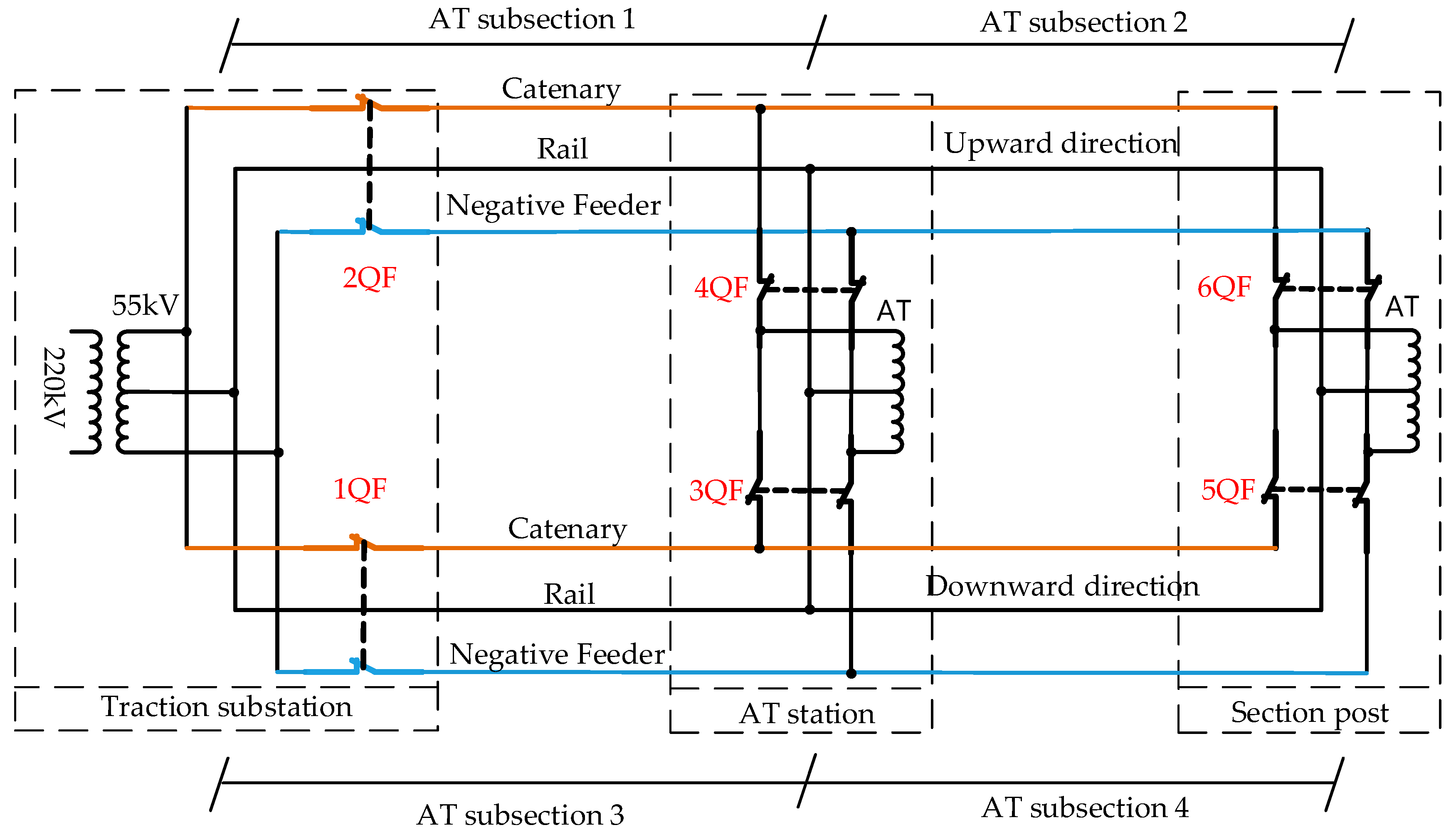
In AT TPSS, the traction substation (TS) delivers energy to EMUs by means of a double wire (catenary and negative feeder) system. The voltage between the catenary and negative feeder is 55 kV. The voltage between the catenary and the rail is 27.5 kV as is the voltage between the rail and the negative feeder. The TPSS is generally delimited as several AT subsections by AT station (ATS). The AT terminals are connected to bus bars of the catenary and negative feeder, whereas its middle winding point is connected to the rail. At the end of the TPSS, another AT station is called the section post (SP), where an AT is connected in a similar way [5,6].
All parallel AT TPSS consists of two AT TPSSs. One of them is described as the upward direction and the other is described as the downward direction. To obtain further feeding ability, the upward direction and downward direction are parallel-connected to the bus bars in the TS, ATS, and SP [7]. In Figure 1, the conventional all parallel AT TPSS with four AT subsections is illustrated. The double pole circuit breakers 1QF and 2QF are connected to the catenary and negative feeder in series in the TS. The AT are connected to the catenary and negative feeder though the double pole circuit breakers 3QF and 4QF in the ATS. Through the connection of the circuit breakers 5QF and 6QF, the AT in the SP has the same installation structure as the AT in the ATS [8].
However, compared to 1 × 25 kV TPSS, the structure of all parallel AT TPSS becomes more complex and is vulnerable to damage by natural or human factors [9]. The fault types are a series of short circuits between catenary and ground (C-G short circuit fault), between the negative feeder and ground (NF-G short circuit fault), and between catenary and negative feeder (C-NF short circuit fault) [10,11]. From the fault resistance, the fault types are divided into low transition resistance faults and high transition resistance faults. A wide variety of fault types seriously jeopardize the safe operation of the whole TPSS. Thus, identifying the faults in a timely and accurate way, isolating them, and reducing the hazards of rail traffic are particularly significant [12,13].
When any short circuit fault occurs in the all parallel AT TPSS in Figure 1, firstly, the circuit breakers 1QF and 2QF are tripped to interrupt the whole TPSS power. Then, 3QF–6QF are tipped to isolate the AT as a result of the voltage loss protection in the ATS and SP [14]. From the view of reliability, the fault of any part in the wires will cause power outage of the whole TPSS, which is a typical series structure. The reason for this phenomenon is that only the circuit breakers 1QF and 2QF are connected to the wires in series and the circuit breakers 3QF–6QF and the ATs in series are parallel-connected to the wires. Therefore, the installation structure of circuit breakers causes that the conventional all parallel AT TPSS fails to switch each wire at the AT subsections on and off independently.
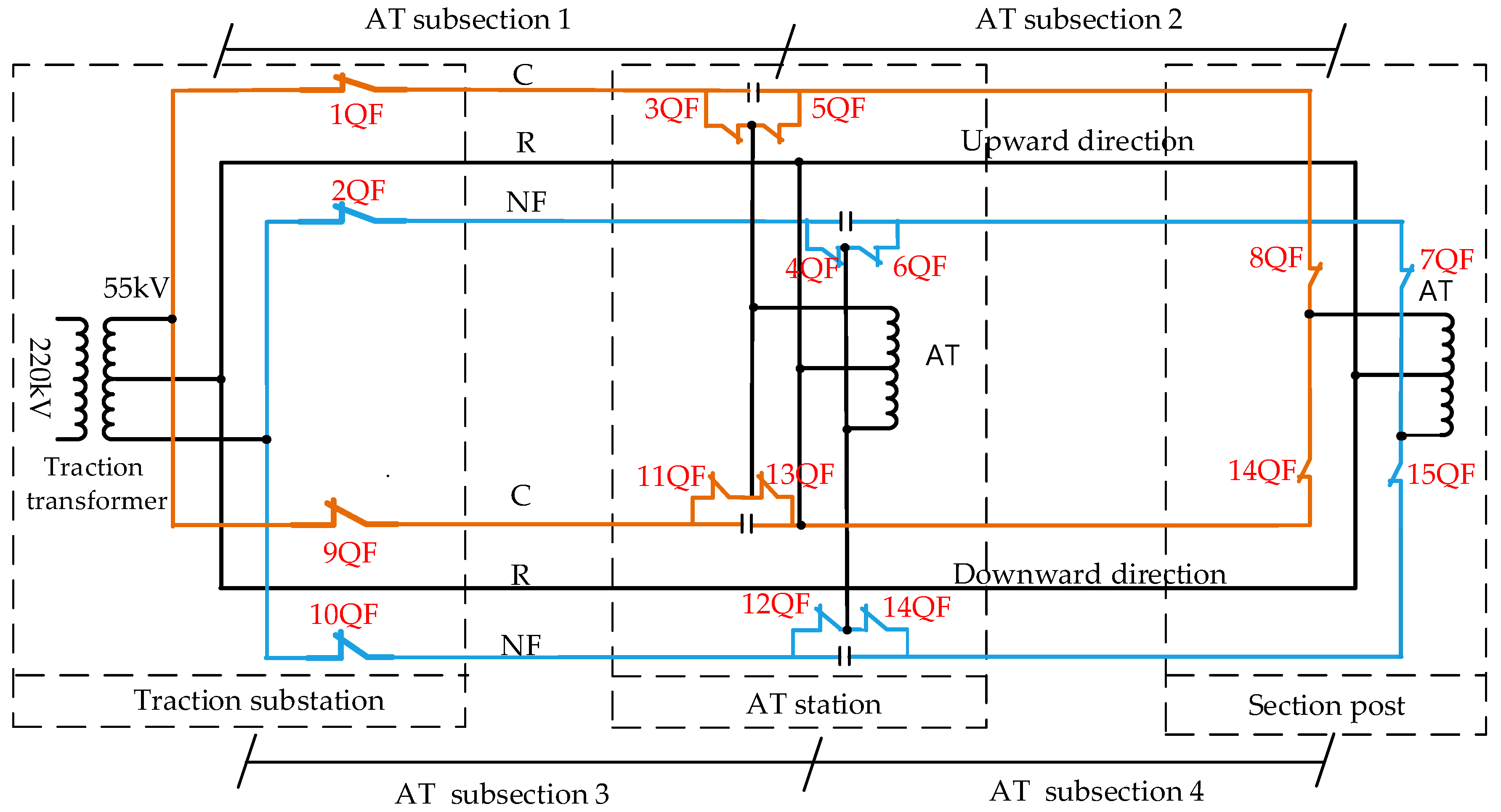
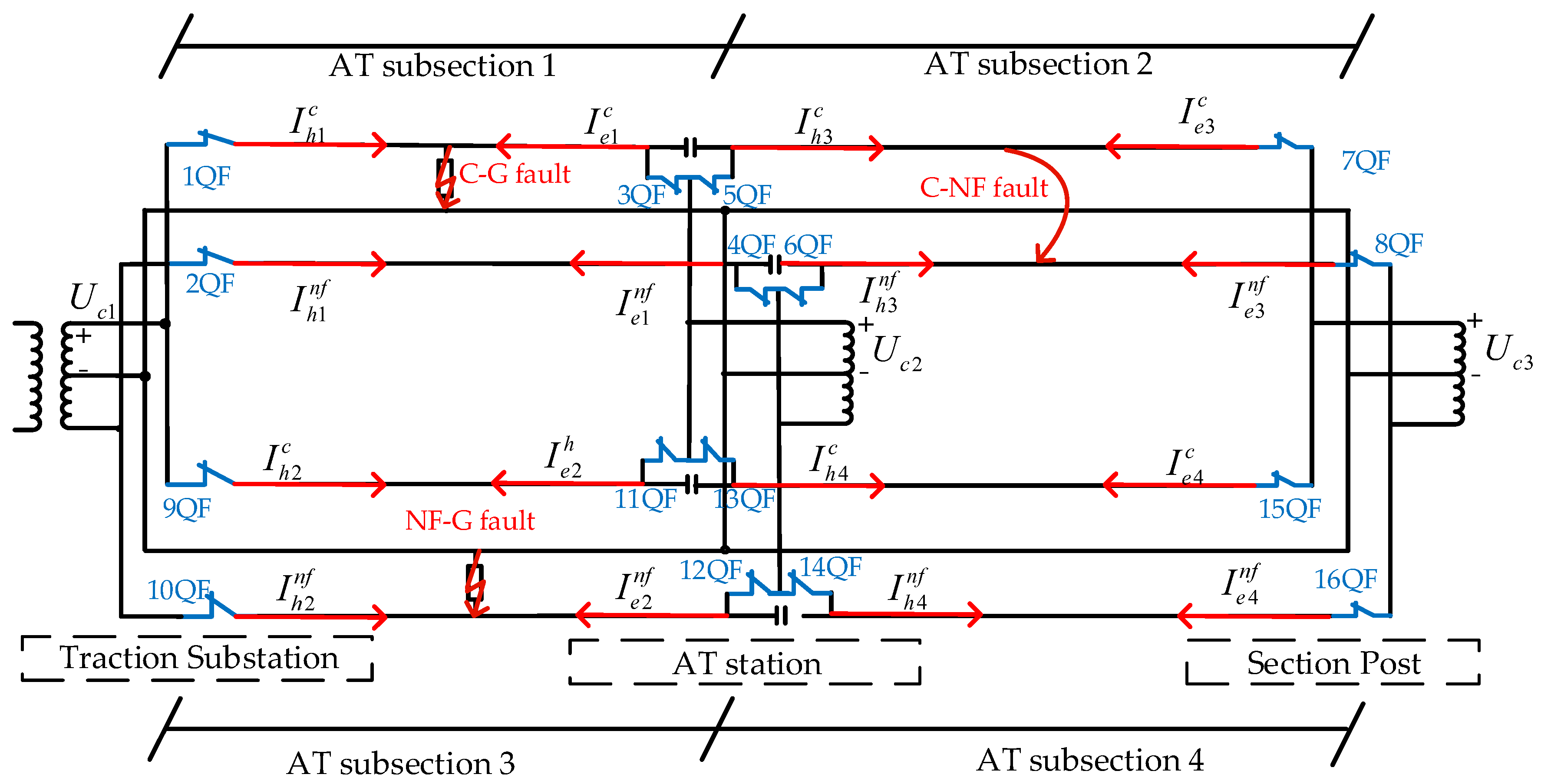
To avoid a fault creating the whole all parallel AT TPSS power outage, a novel segmental power supply scheme is proposed in a past paper [15]. The single-pole circuit breakers are connected to both terminals of the wires at each AT subsection as shown in Figure 2. Each wire could be controlled to switch on or off independently. If the fault type is known, only the wires where the fault is present at the subsection will be quickly removed from service, other subsections remain in service. Compared to the conventional structure of all parallel AT TPSS, the novel scheme imposes only a minimum hazard to rail traffic after the fault occurs [16]. Therefore, the application of this scheme will immensely improve the reliability of all parallel AT TPPS.
The most widely used protection scheme of all parallel AT TPSS is based on single terminal impedance which was developed from 1 × 25 kV TPSS [11,17,18]. In this scheme, distance relays are merely installed in the TS; one-terminal measuring impendence is used to identify fault [14]. On the one hand, due to the widespread nature of ATs, the relationship between impedance and distance in the wire-ground fault is nonlinear [19]. As a result, it is impossible to define the fault subsection when only the impedance is known [20]. On the other hand, due to the symmetry between the C-G fault and NF-G fault, the distance relays lack the ability to figure out fault types [6,21]. In a past paper [22], distance relays are installed in the TS, ATS, and SP to identify the fault subsection. Nevertheless, fault types are still not identified by multiterminals measuring impendence. In addition, with the increase of EMU power, the measuring impedance decreased [15,23] and the resistance set parameter of the high-speed railway becomes smaller. The ability of distance relays to avoid transition resistance is weakened, which threatens the safety operation of the TPSS.
For reduction of the power outage range, the method is proposed to identify and isolate the fault direction [24]. In this method, the current ratio of the upward direction and downward direction in TS is applied. When the fault occurs at AT subsection 1 and AT subsection 3, this method is useful. However, when the fault occurs at other subsections, this method must be combined with the directional overcurrent relays installed in the ATS and SP to identify the fault.
In another past paper [20], the method can identify the C-G fault and NF-G fault at the AT subsection. In this method, the current distribution under normal operation was regarded as the resistive load case, the short circuit current is similar to the inductive load case. The angles between the current and voltage, which are measured by the directional overcurrent relays installed in TS, ATS, and SP, serve to identify the fault. Unfortunately, the C-NF fault and how to isolate the wires and subsections are not mentioned.
An identification method based on segmental scheme is put forward in a previous work [25]. Fault subsections and fault types can be distinguished by the power flow of both terminals of wires at each subsection. However, the high transition resistance fault is ignored and not discussed.
Table 1 lists these studies and compares the covered technologies, their functions, and the structure of TPSS.
In this paper, based on the segmental power supply scheme, the electrical characteristics distribution of all parallel AT TPSS is analyzed, and the new hybrid fault identification method with multiterminals synchronous measure information is described. The method allows an upper device, which analyzes the electrical information uploaded from the bottom devices, to identify the wires where the fault occurs in the AT subsection. After the fault is identified, the wires at the subsection are isolated independently; hence the impact of the fault is limited to a small degree. Accordingly, the safety and reliability of the TPSS can be improved significantly.
The rest of the paper is organized as follows. Section 2 details electrical characteristics of all parallel AT TPSS, Section 3 shows the principles of the proposed hybrid fault identification method, Section 4 presents the analysis of the simulations developed with MATLAB® software (The MathWorks, Inc. 3 Apple Hill Drive Natick, MA, USA), and Section 5 presents the results of the experimental tests carried out in the laboratory. Finally, Section 6 concludes with the main contributions of the proposed method and the direction of future work.

2. Theoretical Analysis of the Current and Voltage Distribution
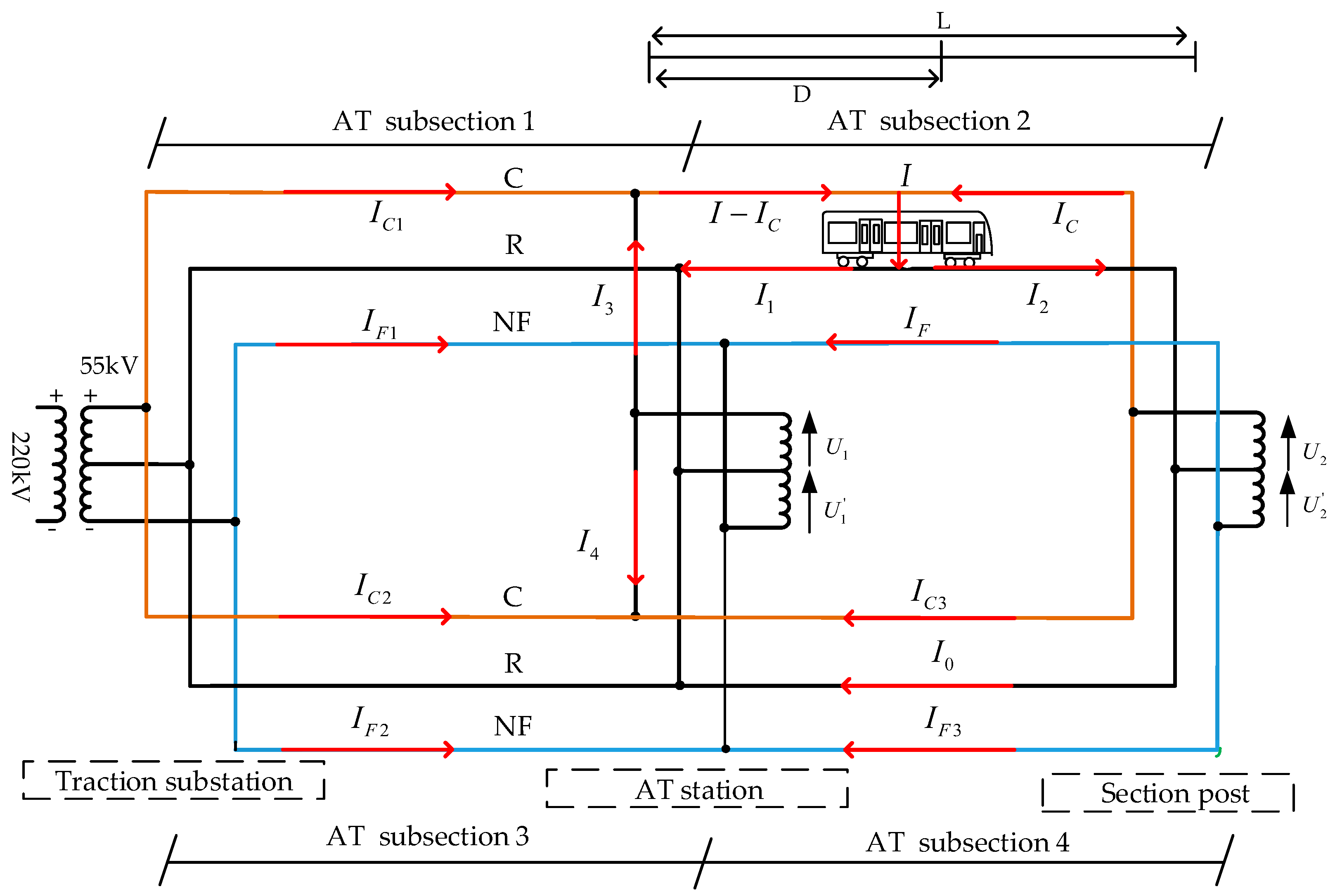
In Figure 3, an EMU is delivered energy from the catenary through the pantograph at subsection 2. The distance from the EMU to the ATS is D km while the total distance of the second subsection is L km. Z C , Z R , and Z N F are the self-impedance value per length unit of catenary, rail, and negative feeder, respectively. Z C R , Z N F R , and Z C N F are the mutual-impedance value per length unit between them.
When the AT leakage impedance and the unsymmetrical distribution of the catenary and negative feeder impedance are ignored, some equations can be obtained:
{ I C 1 = I I C I 3 I C 2 = I C 3 I 4 I 1 = 2 ( I 3 + I 4 ) I C 3 = 1 2 ( I 2 I 0 ) I C I F 3 = 1 2 ( I 2 I 0 ) I F I C 1 = I C 2 = I F 2 = I F 1 U 1 U 2 = U 1 U 2  
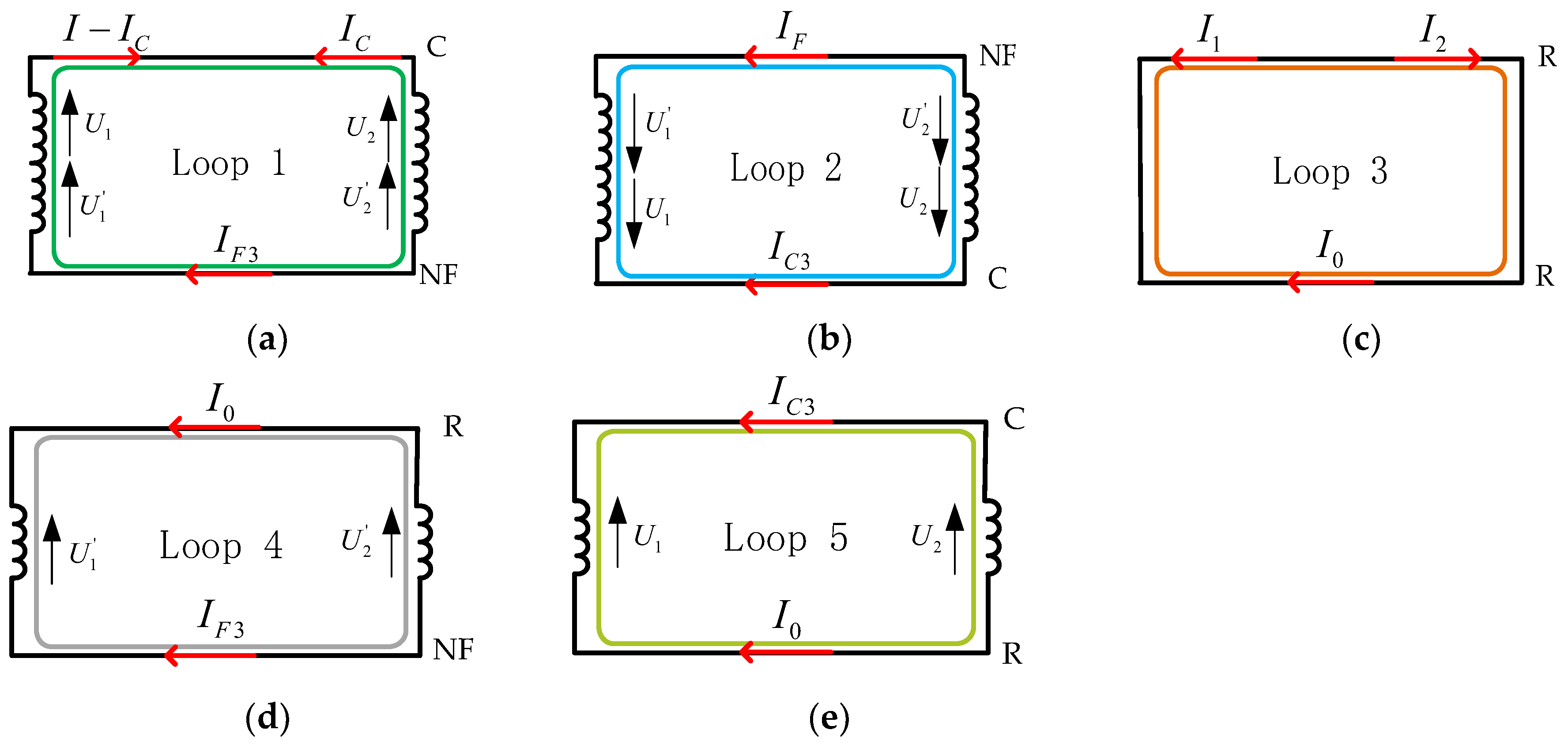
By analyzing the current loops in Figure 4, the five loop current equations can be described:
Loop 1:
( D I L I c ) Z c U 2 U 2 + L I F 3 Z N F + U 1 + U 1 + ( L I 2 D I 2 D I 1 ) Z C R ( L I F L I C 3 ) Z C N F + L I 0 Z R N F = 0  
Loop 2:
L I F Z N F + U 2 + U 2 + L I C 3 Z C U 1 U 1 + ( D I L I C + L I F 3 ) Z C N F + L I 0 Z C R + ( L I 2 D I 2 D I 1 ) Z N F R = 0  
Loop 3:
( D I 1 + L I 2 D I 2 + L I 0 ) Z R + ( D I L I c + L I c 3 ) Z C R + ( L I F 3 L I F ) Z N F R = 0  
Loop 4:
I C 3 Z C + I 0 Z R + Z C R ( I C 3 I 0 ) + I F 3 Z N F R + I F 3 Z C N F U 1 + U 2 = 0  
Loop 5:
I F 3 Z N F I 0 Z R I F 3 Z N F R I C 3 Z C R + I C 3 Z C N F + I 0 Z N F R + U 1 U 2 = 0  
The current distribution equation can be obtained from Equations (1)–(6) as follows,
{ I C = 3 D 4 L I I F = I F 3 = I C 3 = D 4 L I I C 1 = I C 2 = I F 1 = I F 2 = 1 4 I  
Due to the symmetry between the subsections, when an EMU is running at another subsection, a similar current distribution can be obtained.
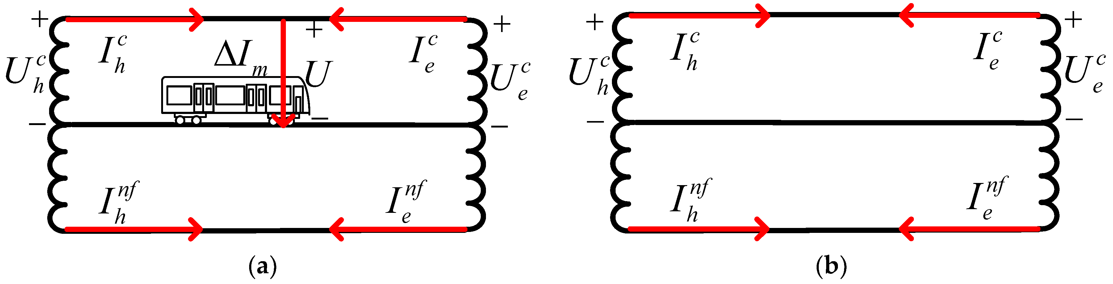
In an AT subsection, the terminal near the TS is called the head terminal, h , and the remote terminal is the end terminal e . In Figure 5, the current in the head terminal of the catenary is given by I h c , and in the end terminal is given by I e c . Similarly, the currents in negative feeder are I h n f and I e n f . Similarly, the catenary voltages are U h c and U e c .
The fundamental wave of current at the present time, I t 2 , and the fundamental wave of current at a primitive period ago, I t 1 , are given; the increment current Δ I can be computed as follows,
I t 2 I t 1 = Δ I  
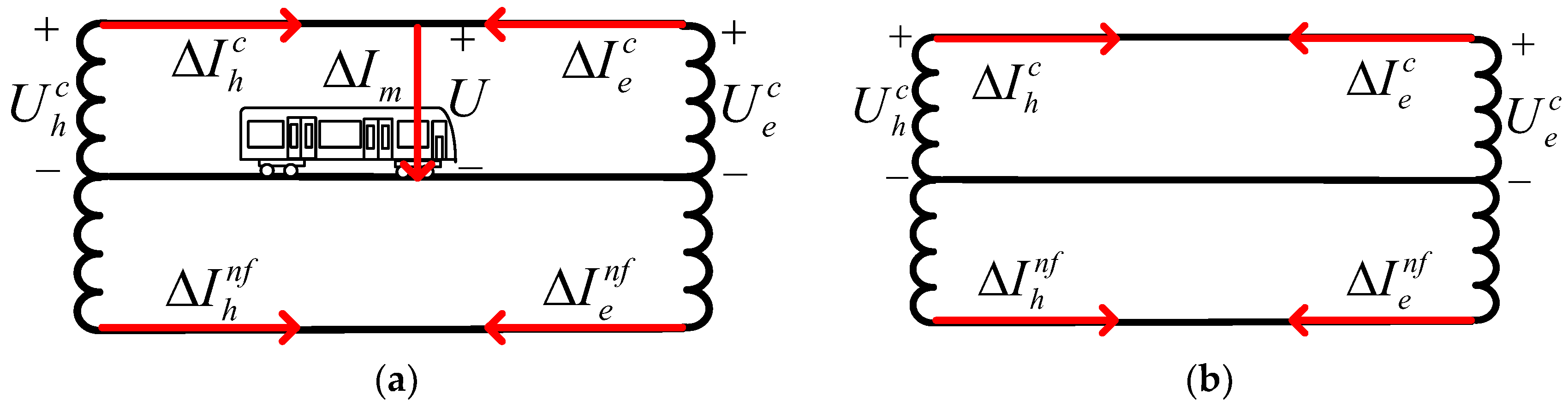
When one EMU is starting, the maximum increment current of the EMU occurs. As EMU start-up time is short, in the vast majority of circumstances, only one EMU is starting in all parallel AT TPSS. If the maximum increment current of the EMU is Δ I m at the AT subsection as Figure 6 shows, with growth of distance, D , derived from Equation (7), the distribution of the maximum increment current at the EMU running subsection can be presented as Equations (9) and (10).
| Δ I h c + Δ I e c | = Δ I m  
| Δ I h n f | = | Δ I e n f | = 1 4 Δ I m  
Similarly, the distribution of the maximum increment current at other subsections can be expressed as:
| Δ I h c | = | Δ I e c | = | Δ I h n f | = | Δ I e n f | = 1 4 Δ I m  
Under normal operation, the increment current of EMUs is not very large. When a short-circuit fault occurs in the TPSS, the short circuit current will increase rapidly. According to whether the increment current of the catenary is larger than that of EMU, the identification method for the high transition resistance short circuit fault can be obtained.
When the voltage root mean square (RMS) | U | of the pantograph drops below the threshold, the voltage will not meet the normal work conditions of the converter in the EMU, so the EMU stops to get energy from the catenary but there is only short circuit current in the TPSS. The pantograph voltage below the threshold and the current distribution can serve to identify the low transition resistance short circuit fault. However, the pantograph voltage cannot be obtained in the TPSS. The catenary voltage U h c and U e c can be used to replace the pantograph voltage.

3. Principles of the Hybrid Fault Identification Method

After analyzing the current and voltage distribution in all parallel AT TPSS, a fault identification method is obtained which regards each AT subsection as a protection unit.
Operation current Δ I o p c and restraint current Δ I r e c can be described as follows [26],
| I h c + I e c | = I o p c  
| I h c I e c | = I r e c  
Operation increment current Δ I o p c and restraint increment current I r e n f can be expressed as follows [27],
| Δ I h c + Δ I e c | = Δ I o p c  
| Δ I h c Δ I e c | = Δ I r e c  
Similarly, operation current I o p n f , restraint current I r e n f , operation increment current Δ I o p n f , and restraint increment current Δ I r e n f in the negative feeder can also be computed.

3.1. Identification Method of Fault with Low Transition Resistance

The preliminary identification of a fault with low transition resistance is given by the following equation,
| U h c | < V   or   | U e c | < V  
where V is the threshold. After a preliminary identification in Equation (16), the confirmed identification equation of the short circuit wires is described as:
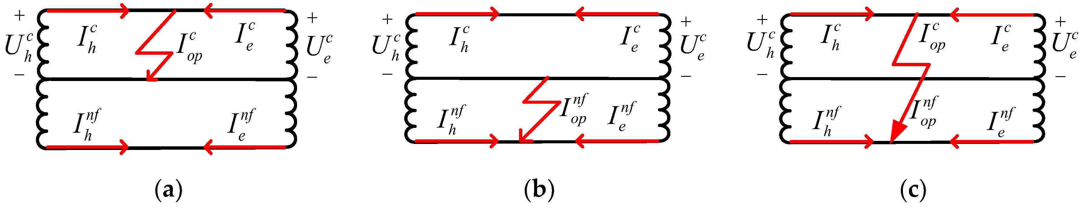
I o p c I s e t   and   I o p c k 1 I r e c  
I o p n f I s e t   and   I o p n f k 1 I r e n f  
where I s e t is the pick-up current and k 1 is the reliability coefficient. As Figure 7 illustrates, the C-G fault is identified when Equations (16) and (17) are satisfied, the NF-G fault is identified if Equations (16) and (18) are satisfied, and the C-NF fault is indicated if the condition of Equations (16)–(18) are set up.

3.2. Identification Method of Fault with High Transition Resistance

3.2.1. Identification of C-G Fault

Derived from Equations (9) and (14), the preliminary identification which indicates if there may be a C-G fault is given by the following equation,
Δ I o p c > k 2 Δ I m  
where k 2 is the reliability coefficient. To avoid multiple EMUs starting at the same time in a few cases, the operation current in the catenary must be guaranteed to not fall during a certain period of time, T . The confirmed identification equation is expressed as,
I o p c I o p b c   and   t T  
where I o p b c is the operation current in the catenary at the moment when the fault occurs, t is the time of I o p c I o p b c , and T 
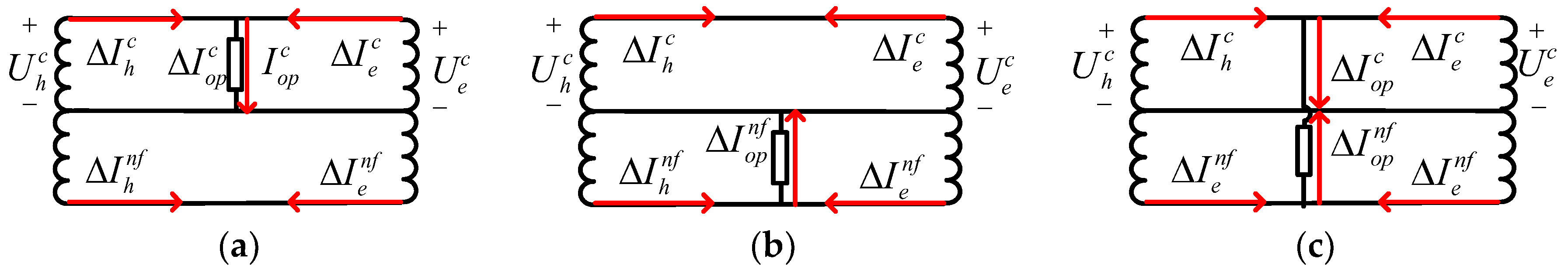
is the pick-up time. The current of EMU will drop after the short EMU start-up time, but the short circuit current will last until the fault is removed; Equation (20) is used to effectively avoid the current caused when multiple EMUs start-up. As Figure 8a shows, the C-G fault is indicated.

3.2.2. Identification of NF-G and C-NF Fault

Derived from Equations (10) and (11), the preliminary identification, which indicates there may be a fault, is obtained by the following equation,
| Δ I h n f | > 1 4 Δ I m   or   | Δ I e n f | > 1 4 Δ I m  
After a preliminary identification in Equation (21), the confirmed identification of the short circuit in the negative feeder can be shown as follows,
Δ I o p n f Δ I s e t n f   and   Δ I o p n f k 3 Δ I r e n f  
where k 3 is the restraint coefficient. After Equation (22) is satisfied, the confirmed identification of the short circuit in the catenary is described as,
Δ I o p n f Δ I o p c Δ I s e t c f  
where Δ I s e t n f and Δ I s e t c f are pick-up increment currents. When Equations (21) and (22) are satisfied the NF-G fault is figured out, as Figure 8b shows. In Equation (23), when the C-NF fault occurs without an EMU at the AT subsection the operation increment current in the catenary and negative feeder are almost equal. However, at the EMU running subsection, as the operation increment current is comprised of the EMU increment current and the fault increment current, the EMU current increases due to the voltage drop of the catenary caused by the fault, so the operation increment current of the catenary is larger than it in the negative feeder. Therefore, if the Equations (21)–(23) are satisfied, the C-NF fault, as Figure 8c indicates, is confirmed.

3.3. Relationship between Two Kinds of Identification Methods

When the catenary voltage RMS is in the range of 29 kV to 17 kV, in China, EMUs can work normally. In cases of short circuit with high transition resistance, the voltage is still in this range. However, the short circuit current increases rapidly, so the increment current of short circuit is larger than that of the EMU. Therefore, Equations (19)–(23), based on increment current, can be used to distinguish the three fault types with high transition resistance at the AT subsection.
When the catenary voltage is below 17 kV, a short circuit with low transition resistance occurs and there is only short circuit current in the TPSS. Equations (16)–(18), based on low voltage and operation current, can be used to identify the fault types at the AT subsection.
In the identification method of high transition resistance fault, the increment current is widely used, but its discriminant window only exists at the moment when the fault occurred. In the identification method of low transition resistance fault, the low voltage and the operation current can continue to distinguish the fault until the fault removal. The two kinds of fault identification methods for low/high transition resistance constitute a complete hybrid fault identification method for all parallel AT TPSS.

3.4. Equipment Composition and Flowchart of Protection System

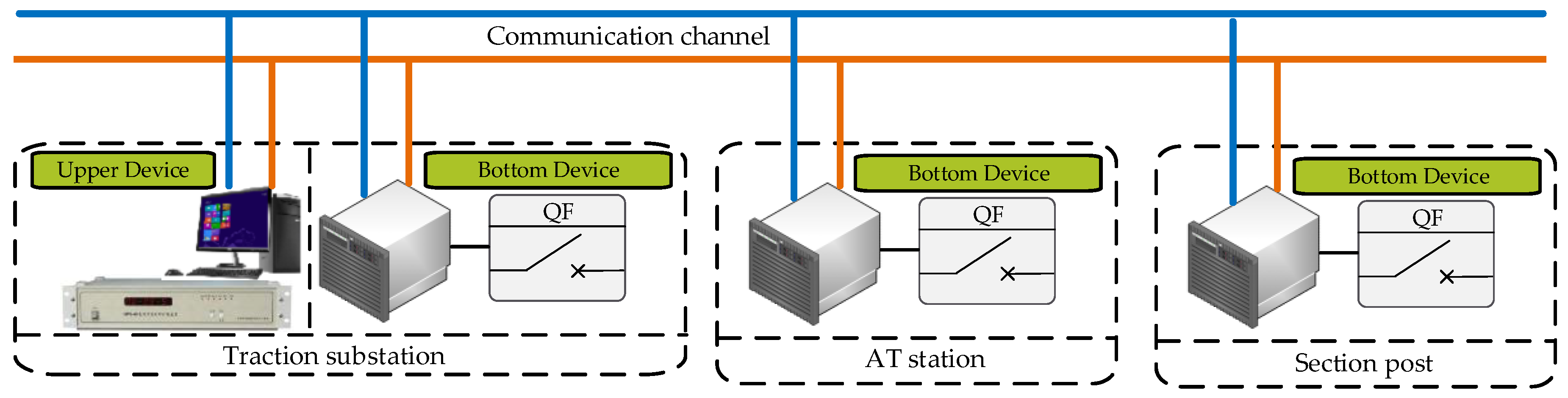
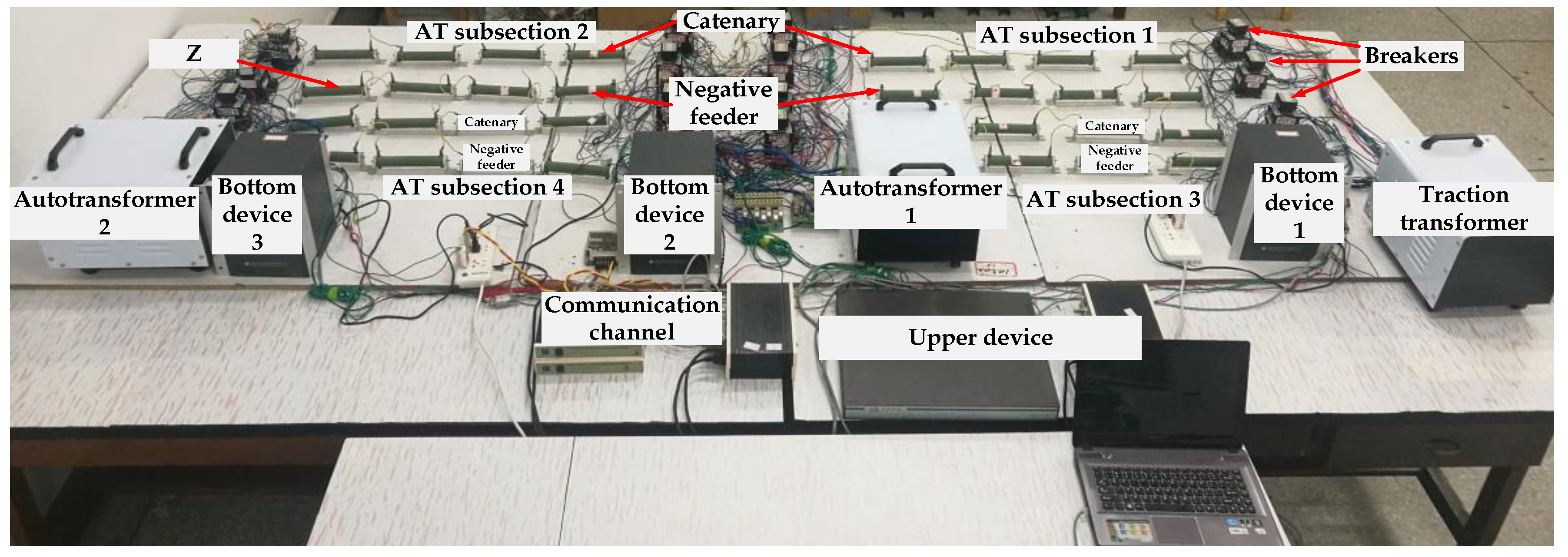
The hybrid fault identification method is realized by means of a protection system mainly composed of the bottom devices, communication channel, and upper device, as shown in Figure 9.
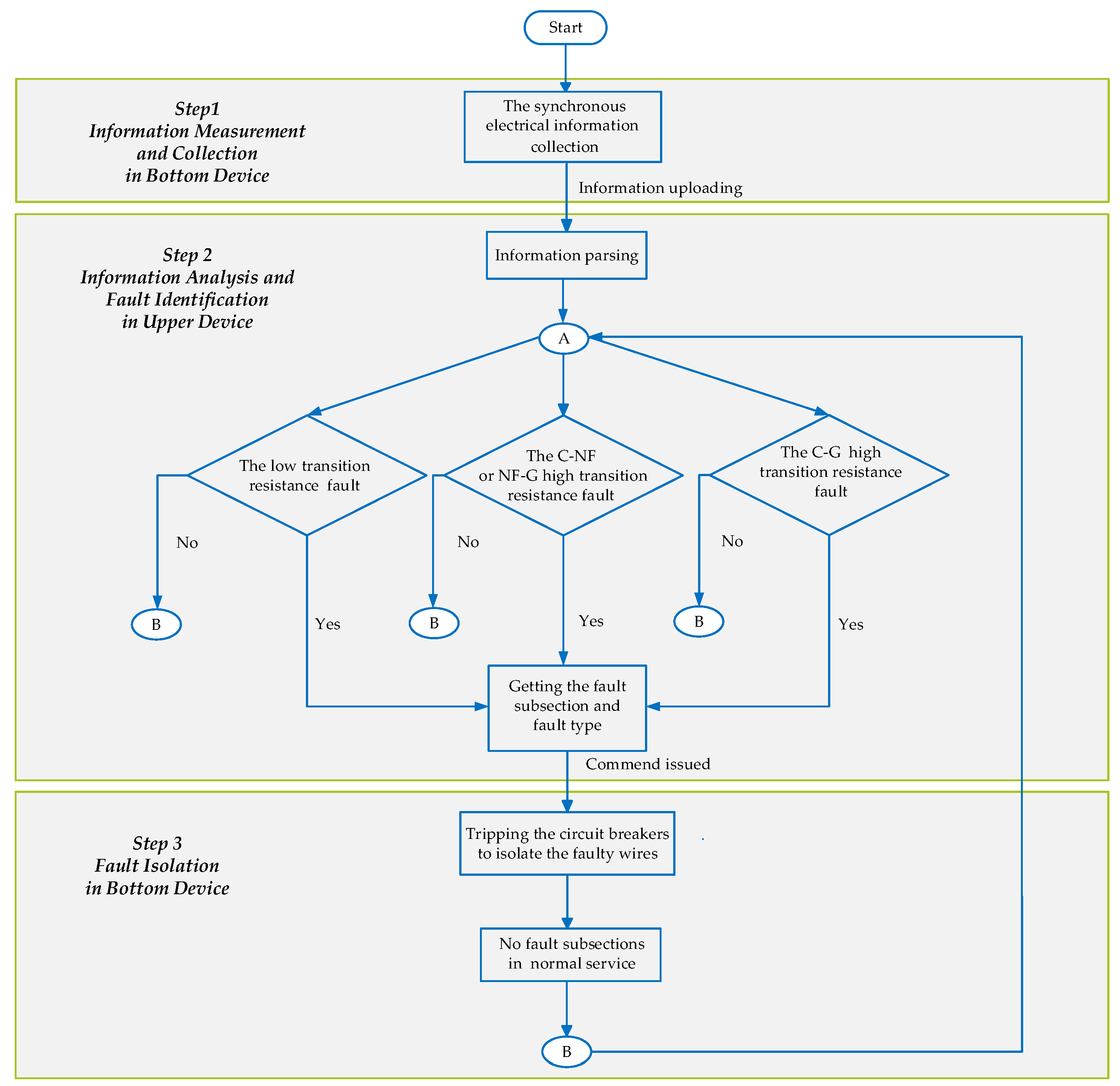
The bottom devices installed in the TS, ATS, and SP are responsible for synchronously collecting the electrical information, uploading real-time information, receiving commands from the upper device, and controlling the circuit breakers. The communication between the bottom devices and the upper device draws support from the fiber channel. The upper device stores and analyzes the electrical information collected from the bottom devices. If a fault occurs, the upper device finds out the fault subsection and fault type by the hybrid fault identification method, the command is issued to the bottom devices to control the circuit breakers to isolate the wires where the fault occurs, so the protection system makes sure that no fault AT subsections work normally. The flowchart of the protection system is presented in Figure 10.
As Figure 9 and Figure 11 show, the bottom devices synchronously collect information include the voltage from TS, ATS and SP ( U c 1 , U c 2 , and U c 3 ), the current of each wire ( I h i c , I e i c , I h i n f and I e i n f ) at the AT subsection i , as well as the state of each circuit breaker in the all parallel TPSS, and upload them to the upper device. When the C-G fault occurs, the upper device can identify the fault details, and sends out a tripping command to the bottom devices in TS and ATS. The bottom devices trip the circuit breakers 1QF and 3QF. Finally, other AT subsections continue in normal operation. Similarly, when the C-NF fault occurs at AT subsection 2, the circuit breakers 5QF, 6QF, 7QF, and 8QF are tripped. If the NF-G fault occurs at AT subsection 3, the circuit breakers 10QF and 12QF are tripped.

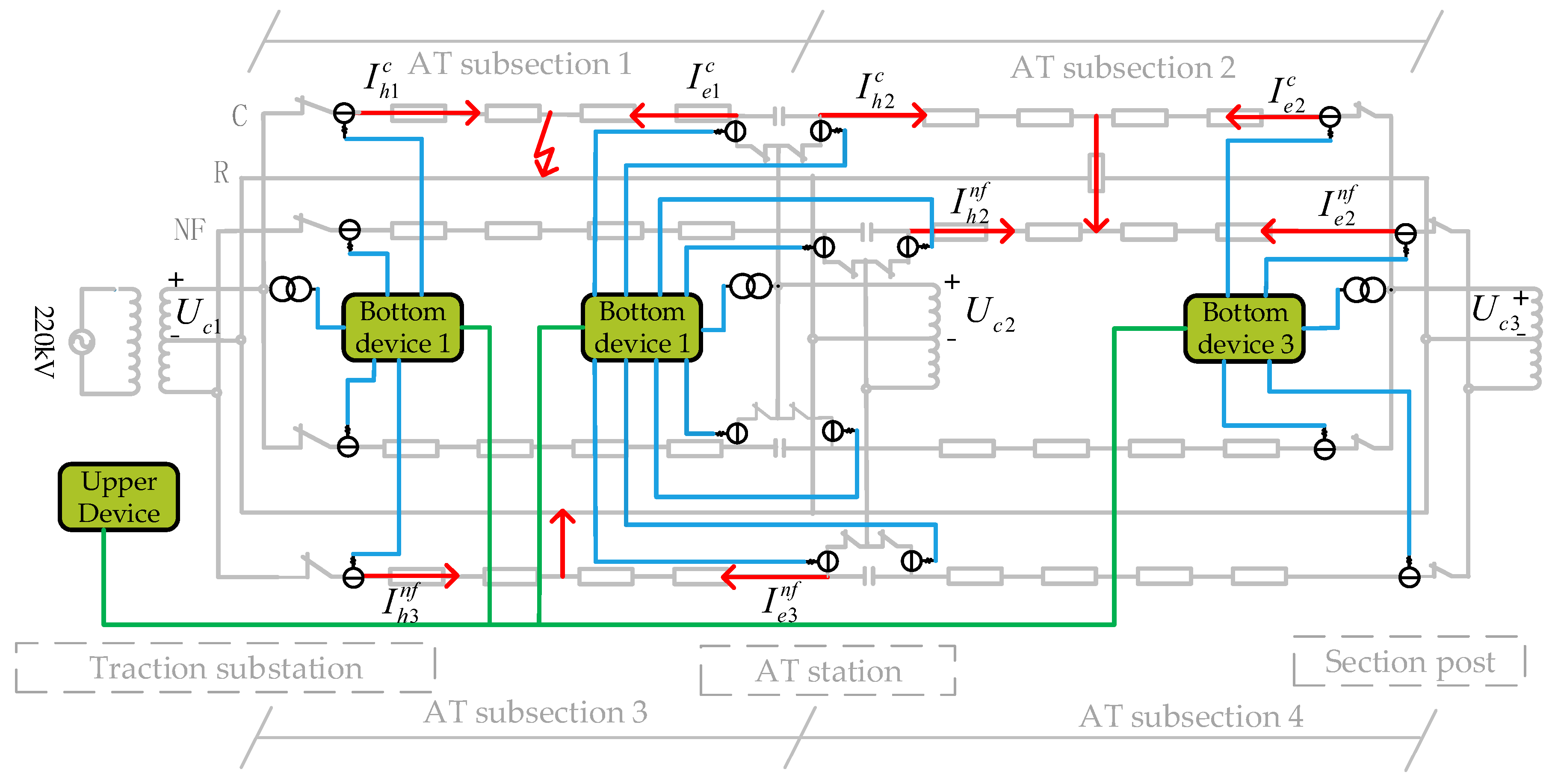
4. Experimental Simulations

In order to verify the validity of the fundamentals of the proposed hybrid fault identification method, a simulation model was constructed using MATLAB® software. The simulation circuit followed the configuration as indicated in 
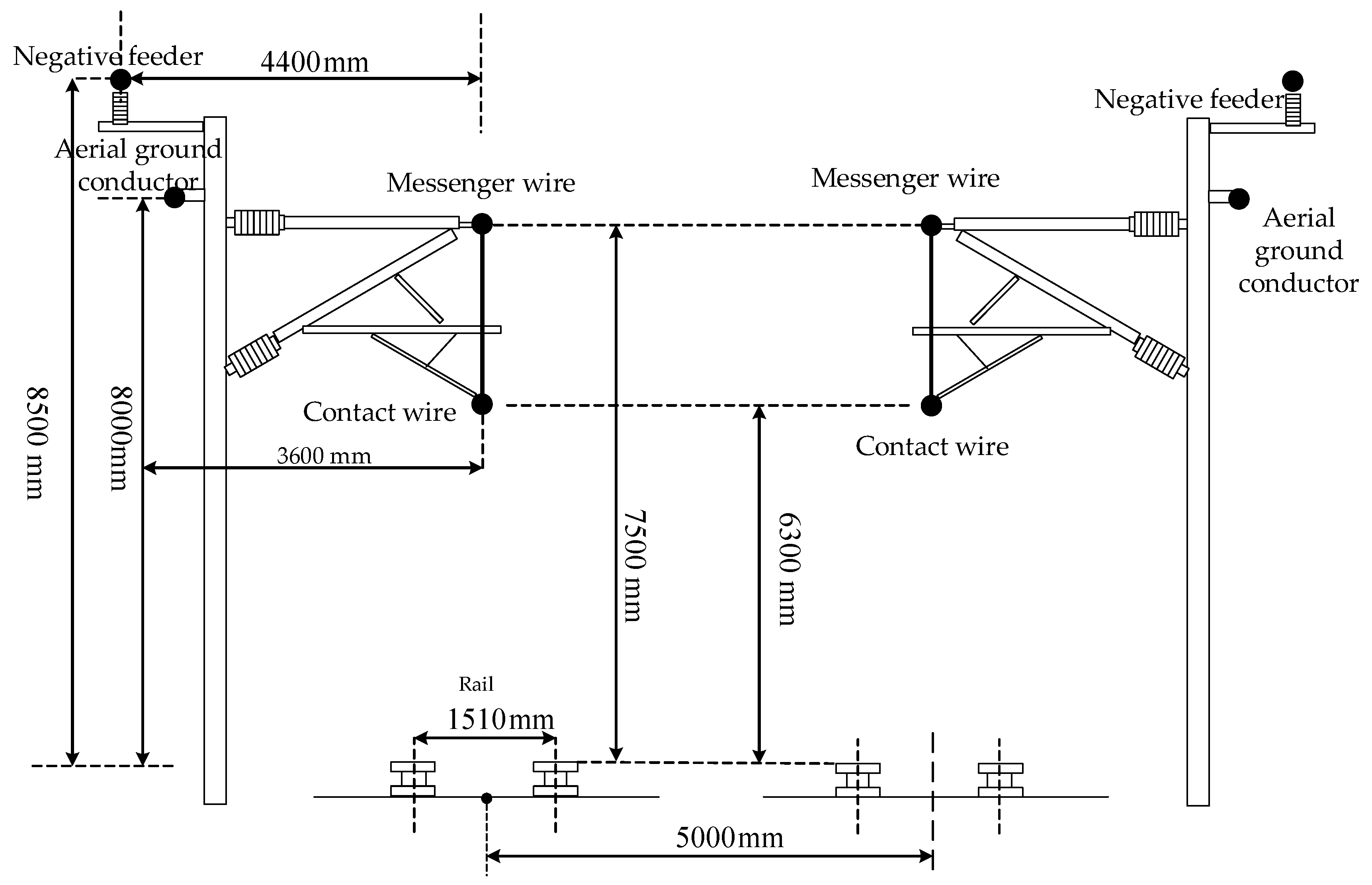
Figure 11. The circuit was supplied by the source of 220 kV and the minimum short circuit capacity was 6704 MVA. The V/x transformer was applied as the traction transformer, which transformed 220 kV to 55 kV, and its rated capacity was 40 MVA. The rated capacity of the AT transformers was 32 MVA. The circuit had four AT subsections and the length of each subsection was 12 km. The impedances parameters of the simulation model were computed from the actual railway of Datong–Xian in China, as shown in Figure 12. The impedances are shown in Table 2.
The fiber channel was ignored in the simulation model, and the bottom devices and the upper device were all realized. The parameters in the upper device are presented in Table 3.
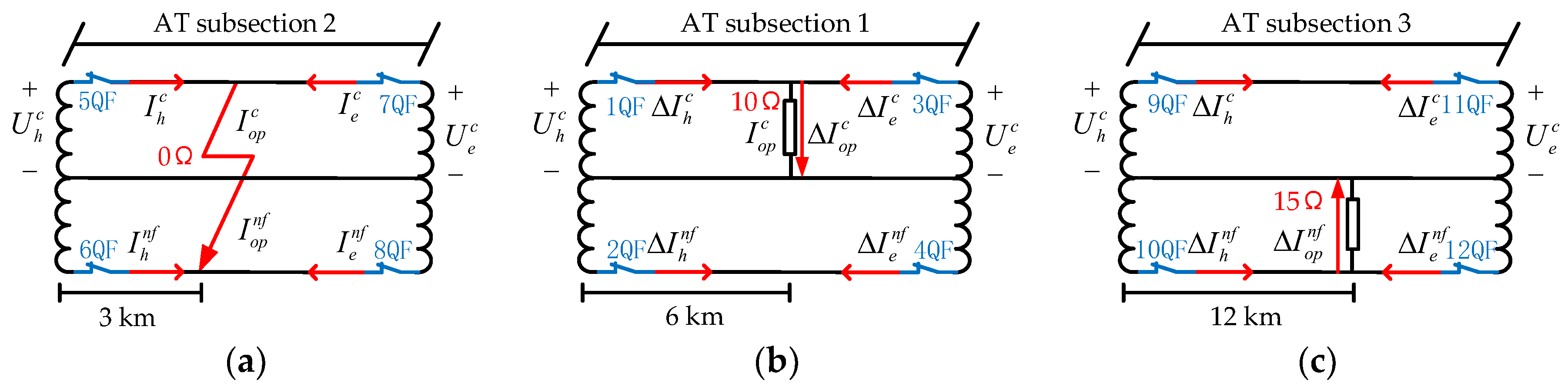
Numerous cases of different transition resistance at different short circuit locations were simulated. In this section, the three typical short circuit faults in three different locations were presented, the C-NF fault at AT subsection 2 in 3 km with 0 Ω transition resistance; the C-G fault at AT subsection 1 in 6 km with 10 Ω; and the NF-G fault at AT subsection 3 in 12 km with 15 Ω, as shown in Figure 13.
In the simulation, the command “1” makes the circuit breakers closed and the command “0” makes the breakers open. When the state signals of breakers are “1”, the breakers are closed. The signals are “0” and the circuit breakers are open. In the cases, the tripping time of breakers are delayed in order to better display electrical characteristics.

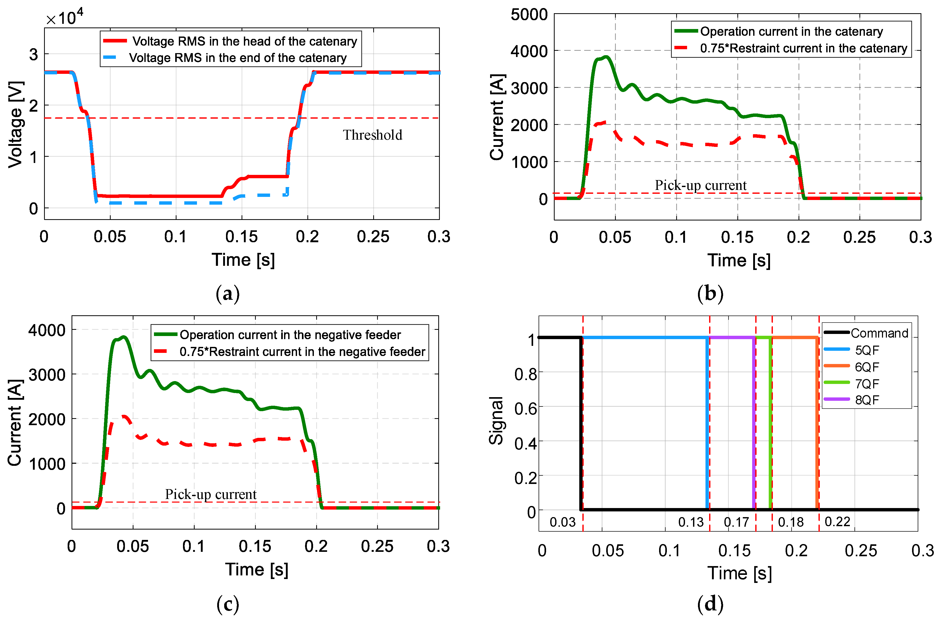
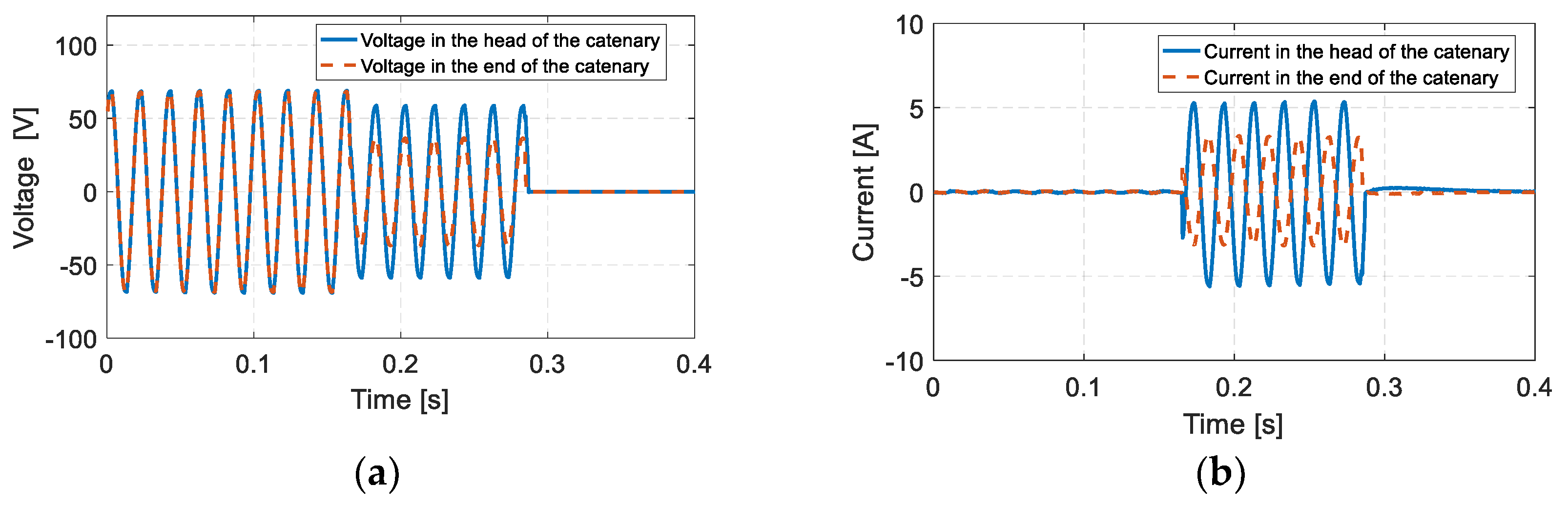
4.1. Case 1: C-NF Fault with 0 Ω Transition Resistance at AT Subsection 2 in 3 km

In the case that a short circuit occurred in Figure 13a at 0.02 s the waveform of the voltage RMS, operation current, restraint current, command, and state of the circuit breakers are presented in Figure 14. The X axes used in Figure 14 are scaled from 0 to 0.2 s; the electrical process of the fault beginning along the fault removal can be observed.
In Figure 14a, when the catenary voltage RMS dropped below the threshold, the upper device preliminarily determined that there was a short circuit with low transition resistance. Moreover, the operation current was greater than the pick-up current and the restraint current in the catenary as well as in the negative feeder as presented in Figure 14b,c. Equations (16)–(18) were satisfied. The upper device determined that the C-NF short circuit occurred at the AT subsection 2 and sent the command to the bottom devices in the ATS and SP at 0.3 s, the circuit breakers was tripped at the different times as Figure 14d shows. Finally, the voltage RMS returned to a normal level, the operation current disappeared, and other subsections kept in service.

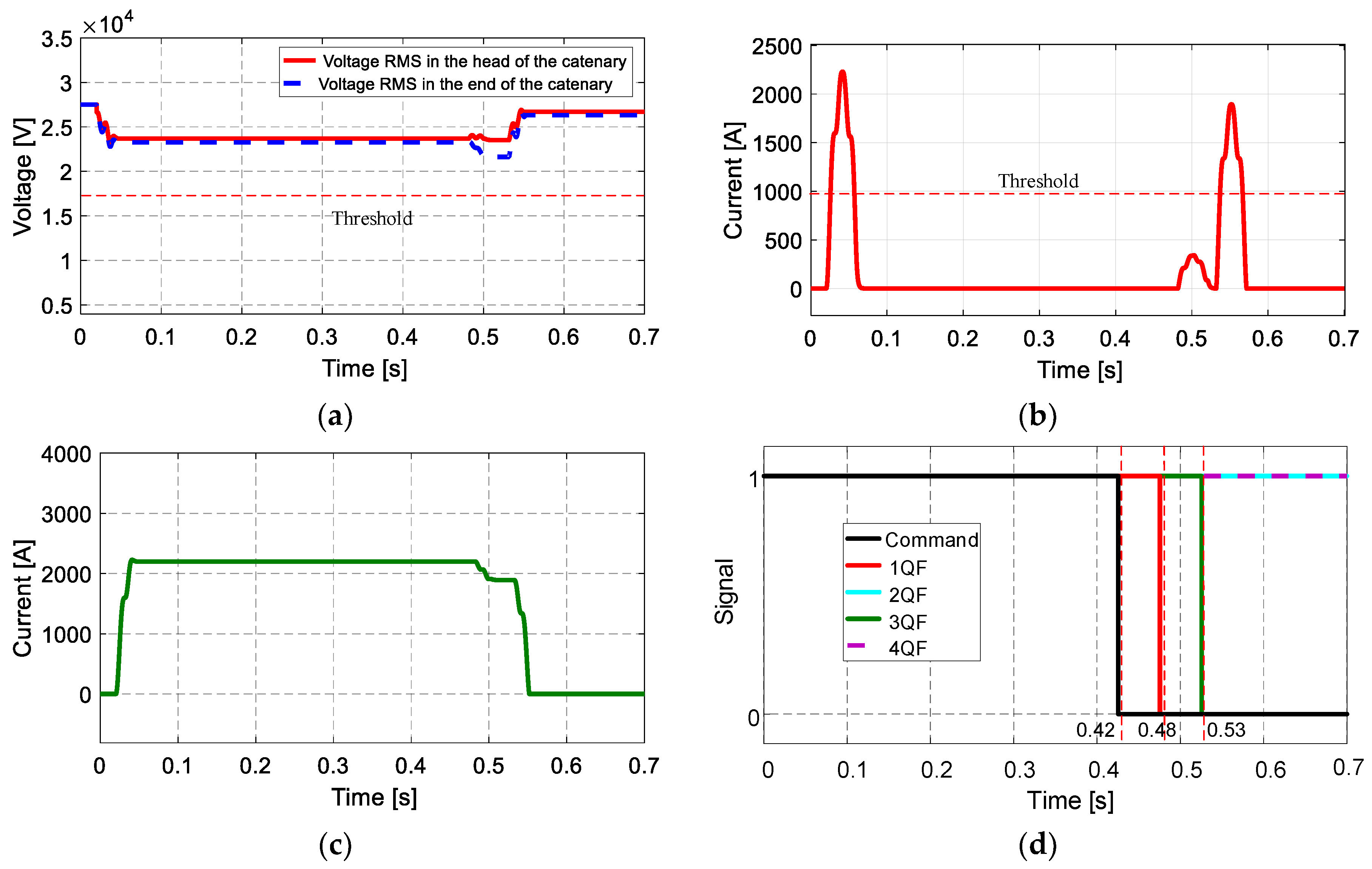
4.2. Case 2: C-G Fualt with 10 Ω Transition Resistance at the AT Subsection 1 in 6 km

A short circuit occurred in Figure 13b at 0.02 s. After the fault occurred, the catenary voltage RMS was still greater than the threshold in Figure 15a. However, the first current crest caused by the short circuit in Figure 15b exceeded the threshold. Furthermore, the operation current continued to not decrease during 0.4 s as Figure 15c shows. Both Equations (19) and (20) were satisfied, the upper device determined that the C-G fault occurred and sent the command to the bottom devices in TS and ATS at 0.42 s, as shown in Figure 15d; the circuit breakers 1QF and 3QF were tripped at different times to disconnect the catenary. Voltage returns to a normal level, the operation increment current displays current crests due to the breakers tripped, and the operation current disappears. The other subsections continued in service.

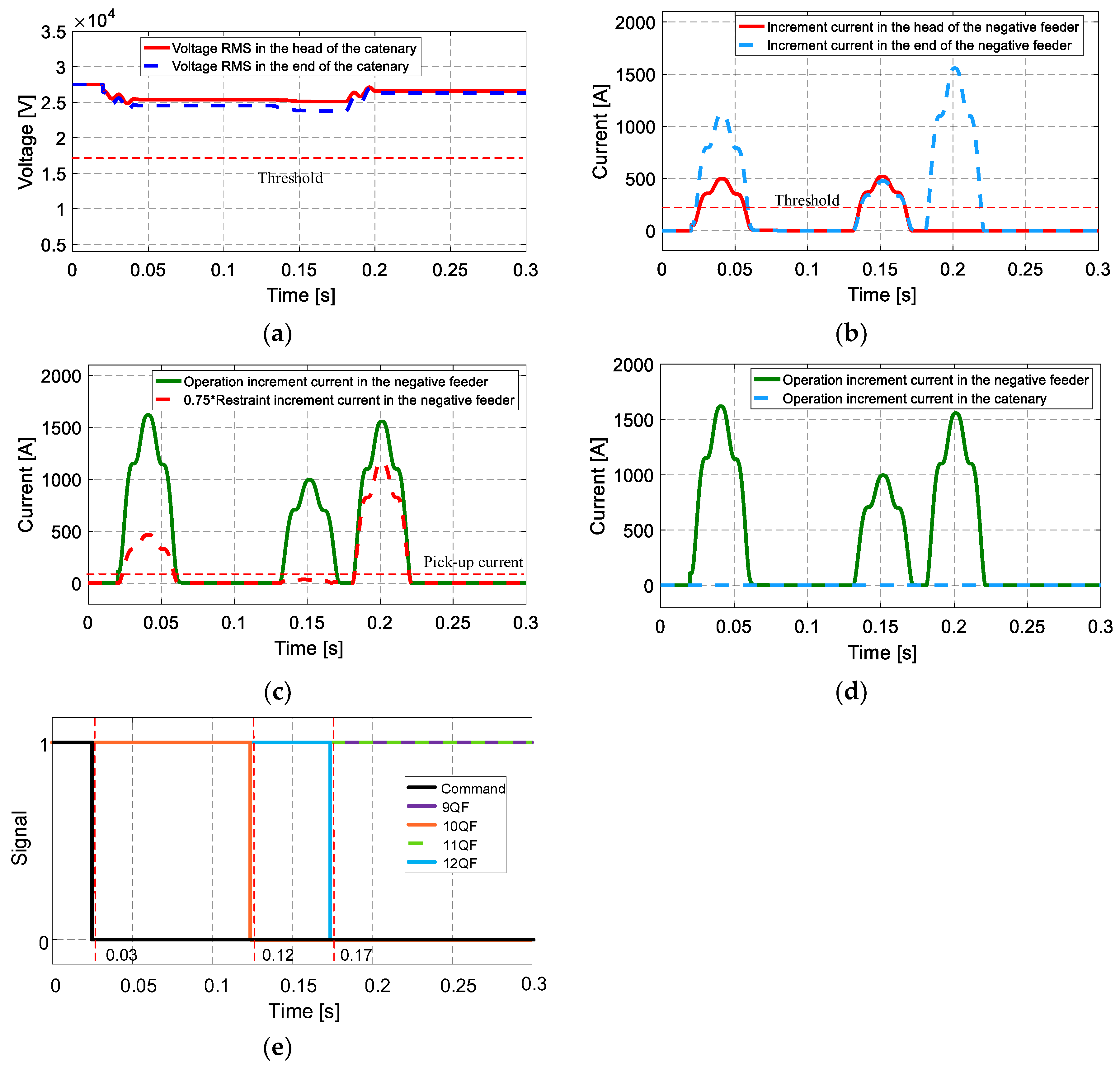
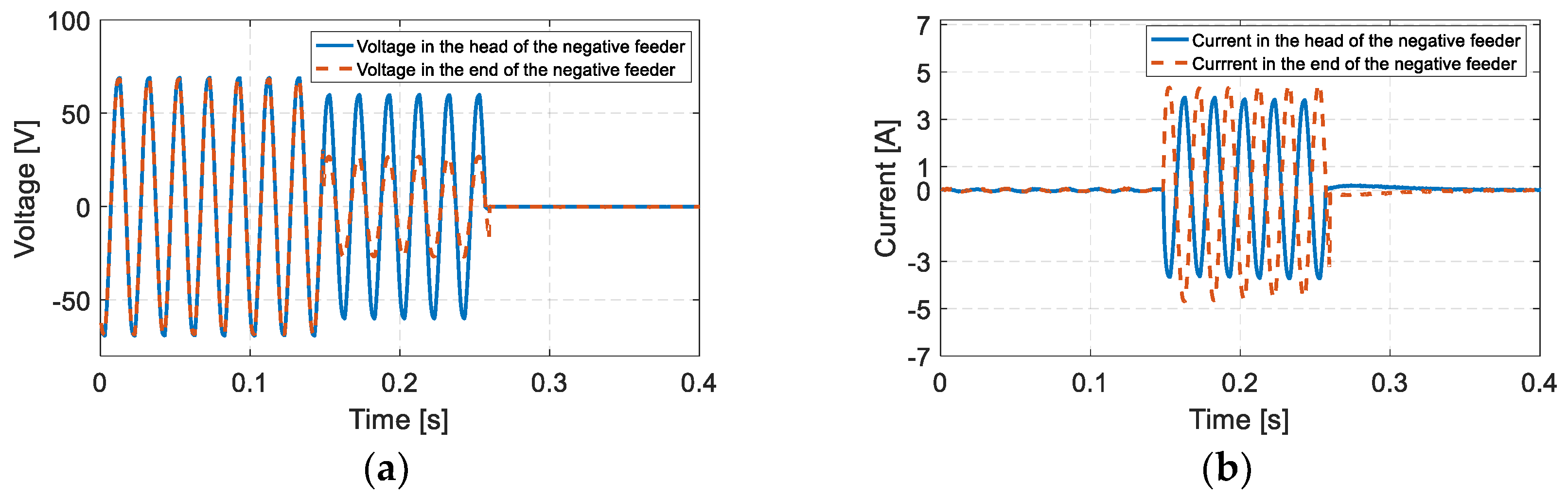
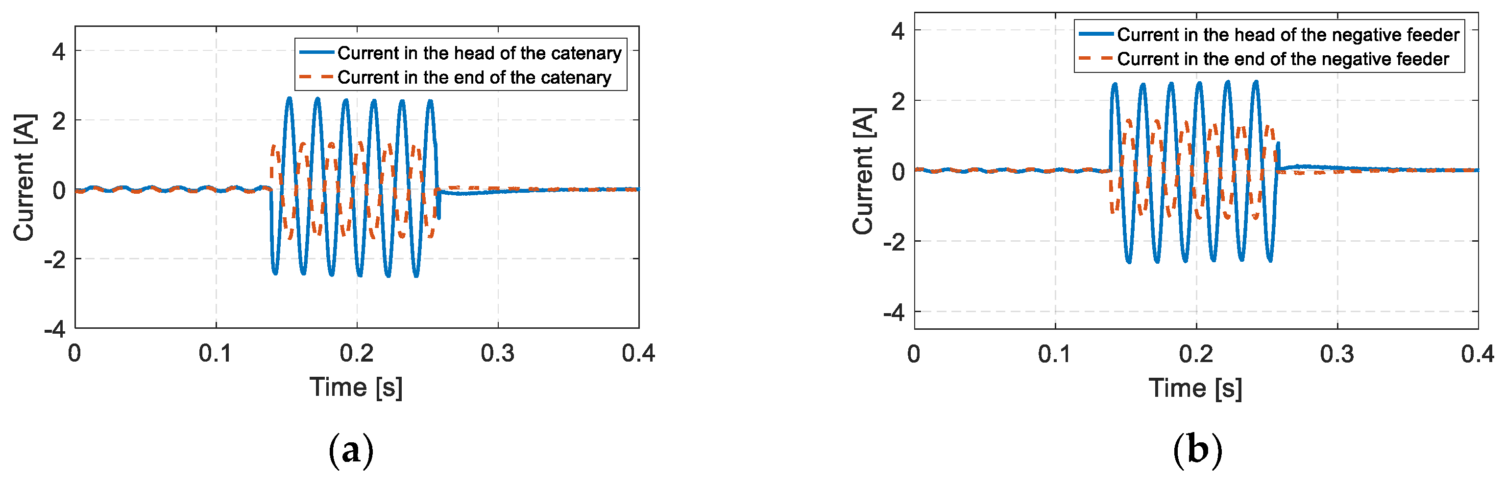
4.3. Case 3: NF-G Fualt with 15 Ω Transition Resistance at the AT Subsection 3 in 12 km

A short circuit occurred in Figure 13c at 0.02 s. After the fault occurred, the catenary voltage RMS dropped, but still was not below the threshold as Figure 16a presents. Whereas the increment current RMS in both terminals of the negative feeder exceeded the threshold as Figure 16b shows, which satisfied Equation (21). Although the operation and restraint increment current in the negative feeder could satisfy Equation (22), but the operation increment current in the catenary and the negative feeder did not satisfy Equation (23), as shown in Figure 16c,d. Finally, the result of NF-G fault was obtained in the upper device, the command was sent at 0.03 s in Figure 16e, the circuit breakers 10QF and 12QF were tripped to disconnect the negative feeder; the catenary at the subsection 3 and other subsections still kept in service.
Through numerous simulations of the different short circuit cases, a new identification method could achieve all the expected goals. It was verified that the method could identify faults correctly and effectively and realize fault removal to the maximum level to keep power supply in all parallel AT TPSS. Therefore, the novel hybrid fault identification method was completely successful.

5. Experimental Laboratory Tests

Aside from the computer simulations, multiple tests were performed in the laboratory with the aim of getting results that allowed for fault identification and fault removal in a practical way. Figure 17 shows the experimental platform. The experimental platform followed the circuit configuration as indicated in Figure 18.
The distributed impedance of the wires was achieved by a series of resistance Z and the voltage regulator supplied 100 V between the catenary and the negative feeder. The TPSS was divided into four AT subsections through ATs. The contactors were parallel-connected to both terminals of the wires at each AT subsection. The contactors in both terminals could maintain the wire connection or excision. Bottom devices were installed to acquire the synchronous multiterminal electrical information and upload the information to the upper device. The upper device was set to release a tripping command to the bottom devices when the electrical information was proven to meet the tripping conditions. Then, the bottom devices kept the contactors opened or closed. The parameters of the identification method in the experimental platform are presented in Table 4.
Using the experimental platform, three fault types which are not shown in the simulations are presented in this section, and the correctness of the fault identification method was further verified.

5.1. Case 1: C-G Fault at the AT Subsection 1 with 0 Ω Transition Resistance

As shown in Figure 18, a short circuit occurred at the AT subsection 1. The voltage and current in both terminals of the catenary at subsection 1 are presented in Figure 19. In the first cycle, after the fault occurred was calculated, voltage RMS, the operation current, and restraint current in the catenary were obtained.
After the fault occurred, the catenary voltage RMS in the head was 41.62 V, and the other voltage RMS was 25.92 V which was below threshold. The operation current was 5.96 A and the restraint current was 1.51 A in the catenary. The voltage and current satisfied the tripping condition in Equations (16) and (17). The C-G short circuit was confirmed. The contactors in two terminals of the catenary at the AT subsection 1 were tripped around 0.27 s.

5.2. Case 2: NF-G Fault at the AT Subsection 3 with 0 Ω Transition Resistance

A short circuit fault occurred at the AT subsection 3 as Figure 18 shows. Figure 20 illustrates the voltage and current in both terminals of the catenary. After the fault occurred, the catenary voltage RMS in the head was 42.28 V, and the catenary voltage RMS of the end terminal was 18.96 V which was below the threshold. The operation current was 5.66 A and the restraint current was 0.48 A in the negative feeder. Equations (16) and (18) were satisfied. The contactors in two terminals of the negative feeder at the AT subsection 3 were tripped around 0.26 s.

5.3. Case 3: C-NF Fault at the AT Subsection 2 with 17 Ω Transition Resistance

A short circuit occurred at the AT subsection 2 in Figure 18. Figure 21 presents current in both terminals of the catenary and the negative feeder. In the negative feeder, the increment current RMS in the head terminal was 1.74 A; it was 0.91 A in the end terminal. Both terminals increment currents’ RMS exceeded the threshold. In the catenary, the operation increment current was 2.67 A and the restraint increment current was 0.79 A. Moreover, the operation increment current was 2.65 A and the restraint increment current was 0.83 A in the negative feeder. Equations (21)–(23) were coincided. The contactors in both terminals of the AT subsection 2 were tripped around 0.26 s.
As observed, in these fault cases, the correct tripping operation was obtained in the experimental results. Therefore, the fundamentals of the new hybrid fault identification method were further validated.

6. Conclusions

The new hybrid fault identification method with multiterminal synchronous electrical information was presented. Based on the segmental power supply scheme, the protection system adopting the hybrid identification method was designed for the low/high transition resistance fault which was verified through simulations and laboratory experiments by the case studies. Compared to the conventional protection schemes, the hybrid fault identification method can accurately identify the fault subsection and fault type, and quickly removed the wires where the short circuit occurs in the AT subsection without having an effect on the normal operation of other subsections, which significantly improves the reliability of power supply in the all parallel AT TPSS.
The method is inseparable from the support of the bottom devices and the upper device which may increase the investment. In the future work, the devices will be applied to the power quality evaluation and fault location, which will be an important part of the intelligent railway.

Author Contributions

S.W. and M.C. proposed the idea, developed the model, and performed the simulation works. M.C., S.W., W.H., and B.W. contributed the experimental platform and wrote the paper. S.W., M.C., and Q.L. were in charge of reviewing and editing the paper. This work was conducted under the supervision of Q.L.

Funding

This research was funded by the National Natural Science Foundation of China (Grant No. 51877182) and the Science and Technology Plan Project of Sichuan Province (Grant No. 2018FZ0107). The APC was funded by the National Natural Science Foundation of China and the Science and Technology Plan Project of Sichuan Province.

Acknowledgments

This research was supported by the CHINA RAILWAY (CR) and First Design and Survey Institute (FDSI) Group Co., Ltd.

Conflicts of Interest

The authors declare no conflict of interest.

Nomenclature

Abbreviations
ATAutotransformer
TPSSTraction power supply system
TSTraction substation
ATSAutotransformer station
SPSection post
C-G faultShort circuit between catenary and ground
NF-G faultShort circuit between negative feeder and ground
C-NF faultShort circuit between catenary and negative feeder
RMSRoot mean square
Parameters
D Distance from the EMU to the AT station
L Total distance of the AT subsection 2
Z C Catenary self-impedance value per length unit
Z R Rail self-impedance value per length unit
Z N F Negative feeder self-impedance value per length unit
Z C R Mutual impedance catenary-rail value per length unit
Z N F R Mutual impedance negative feeder-rail value per length unit
Z C N F Mutual impedance catenary-negative feeder value per length unit
Δ I m Maximum increment current of an EMU
I s e t , Δ I s e t f , Δ I s e t c f Pick-up current
k 1 , k 2 , k 3 Reliability coefficient
V Voltage threshold
T Pick-up time
Variables
I h c , I e c Current in the head and end terminal of catenary
I h n f , I e n f Current in the head and end terminal of negative feeder
I h i c , I e i c Current in the head and end terminal of catenary at the AT subsection i
I h i n f , I e i n f Current in the head and end terminal of negative feeder at the AT subsection i
I o p c , I r e c Operation and restraint current of catenary
I o p n f , I r e n f Operation and restraint current of negative feeder
Δ I o p c , Δ I r e c Operation and restraint increment current of catenary
Δ I o p n f , Δ I r e n f Operation and restraint increment current of negative feeder
U Voltage of pantograph
U h c Voltage of the head terminal of catenary at the AT subsection
U e c Voltage of the end terminal of catenary at the AT subsection
U c 1 Voltage of catenary in the traction substation
U c 2 Voltage of catenary in the AT station
U c 3 Voltage of catenary in the section post

References

  1. Deng, Y.; Huang, K.; Su, D.; Liu, Z. Spatial magnetic-field description method aimed at 2 × 25 kv auto-transformer power supply system in high-speed railway. Appl. Sci. 2018, 8, 997. [Google Scholar] [CrossRef]
  2. Hemmer, B.; Mariscotti, A.; Wuergler, D. Recommendations for the calculation of the total disturbing return current from electric traction vehicles. IEEE Trans. Power Deliv. 2004, 19, 1190–1197. [Google Scholar] [CrossRef]
  3. Cella, R.; Giangaspero, G.; Mariscotti, A.; Montepagano, A.; Pozzobon, P.; Ruscelli, M.; Vanti, M. Measurement of at electric railway system currents at power-supply frequency and validation of a multiconductor transmission-line model. IEEE Trans. Power Deliv. 2006, 21, 1721–1726. [Google Scholar] [CrossRef]
  4. China National Development and Reform Commission. Mid-Long Term Railway Network Plan. 2016; p. 6. Available online: http://www.ndrc.gov.cn (accessed on 1 October 2018).
  5. Soler-Nicolau, M.; Mera, J.M.; López, J.; Cano-Moreno, J.D. Improving power supply design for high speed lines and 2 × 25 systems using a genetic algorithm. Int. J. Electr. Power Energy Syst. 2018, 99, 309–322. [Google Scholar] [CrossRef]
  6. Gao, Z.; Wang, J.; He, Z. The simulation of T-F short-circuit fault location in all parallel at traction power supply system based on the subsection impedance method. In Proceedings of the Power and Energy Engineering Conference, Shanghai, China, 27–29 March 2012. [Google Scholar] [CrossRef]
  7. Battistelli, L.; Pagano, M.; Proto, D. 2 × 25 kv 50 Hz high-speed traction power system: Short-circuit modeling. IEEE Trans. Power Deliv. 2011, 26, 1459–1466. [Google Scholar] [CrossRef]
  8. Zhao, T.; Wu, M. Electric power characteristics of all-parallel at traction power supply system. In Proceedings of the International Conference on Transportation, Mechanical, and Electrical Engineering, Chengdu, China, 16–18 December 2011. [Google Scholar] [CrossRef]
  9. Wang, C.; Yin, X. Comprehensive revisions on fault-location algorithm suitable for dedicated passenger line of high-speed electrified railway. IEEE Trans. Power Deliv. 2012, 27, 2415–2417. [Google Scholar] [CrossRef]
  10. Chen, T.H.; Hsu, Y.F. Systematized short-circuit analysis of a 2 × 25 kv electric traction network. Electr. Power Syst. Res. 1998, 47, 133–142. [Google Scholar] [CrossRef]
  11. Sezi, T.; Menter, F.E. Protection scheme for a new ac railway traction power system. In Proceedings of the Transmission and Distribution Conference, New Orleans, LA, USA, 11–16 April 1999. [Google Scholar] [CrossRef]
  12. Xu, G.; Zhou, Y.; Chen, Y. Model-based fault location with frequency domain for power traction system. Energies 2013, 6, 3097–3114. [Google Scholar] [CrossRef]
  13. Zhou, Y.; Xu, G.; Chen, Y. Fault location in power electrical traction line system. Energies 2012, 5, 5002–5018. [Google Scholar] [CrossRef]
  14. Han, Z.; Liu, S.; Gao, S.; Bo, Z. Protection scheme for china high-speed railway. In Proceedings of the IET International Conference on Developments in Power System Protection, Manchester, UK, 29 March–1 April 2010. [Google Scholar] [CrossRef]
  15. Li, Q. New generation traction power supply system and its key technologies for electrified railways. J. Mod. Transp. 2015, 23. [Google Scholar] [CrossRef]
  16. Li, Q. Industrial frequency single-phase ac traction power supply system for urban rail transit and its key technologies. J. Mod. Transp. 2016, 24, 103–113. [Google Scholar] [CrossRef]
  17. Gao, S.; Chen, W.; Chen, X. Automation of Traction Power Supply for Passenger Dedicated Line, 2nd ed.; Southwest Jiao Tong University Press: Chengdu, China, 2012; pp. 23–56. ISBN 978-7-5643-1012-7. [Google Scholar]
  18. Huang, Y.; Cai, Y.; Xiao, J.; Tang, L.; Li, J. Research of implementing least squares in digital distance relaying for AC electrified railway. In Proceedings of the IEE International Conference on Developments in Power System Protection, Amsterdam, The Netherlands, 5–8 April 2004; Volume 1, pp. 116–118. [Google Scholar] [CrossRef]
  19. Cho, G.; Ryu, K.; Lee, H.; Heo, S.; Kim, H.; Kim, C.; Kwon, S. A study on the distance relay operation characteristics for korean single track AC electrical railway system. In Proceedings of the International Conference on Development in Power System Protection, Edinburgh, UK, 7–10 March 2016. [Google Scholar] [CrossRef]
  20. Serrano, J.; Platero, C.A.; Lópeztoledo, M.; Granizo, R. A novel ground fault identification method for 2 × 5 kv railway power supply systems. Energies 2015, 8, 7020–7039. [Google Scholar] [CrossRef] [Green Version]
  21. Millard, A.; Taylor, I.A.; Weller, G.C. AC electrified railways-protection and distance to fault measurement. In Proceedings of the International Conference on Electric Railways in A United Europe, Amsterdam, The Netherlands, 27–30 March 1995. [Google Scholar] [CrossRef]
  22. Chen, H.; Xiong, L.; Wang, C. Protection configuration of longitudinal segmented all parallel at traction network. Proc. CSU-EPSA 2015, 27, 47–51. [Google Scholar] [CrossRef]
  23. Chen, M.; Li, Q.; Roberts, C.; Hillmansen, S. Modelling and performance analysis of advanced combined co-phase traction power supply system in electrified railway. IET Gener. Transm. Distrib. 2016, 10, 906–916. [Google Scholar] [CrossRef]
  24. Liu, S.; Han, Z.; Gao, S. Inter-tripping protection scheme for feeding sections of high-speed railway based on current features. J. Chin. Electr. Eng. Sci. 2014, 34, 4437–4442. [Google Scholar] [CrossRef]
  25. Wang, X.; Li, Q.; Chen, M.; Yi, D.; Cui, Z. A scheme of state measure and control of all-parallel at traction network for high-speed railway and simulation analysis. Power Syst. Protect. Control 2016. [Google Scholar] [CrossRef]
  26. Dambhare, S.; Soman, S.A.; Chandorkar, M.C. Adaptive current differential protection schemes for transmission-line protection. IEEE Trans. Power Deliv. 2009, 24, 1832–1841. [Google Scholar] [CrossRef]
  27. Li, X.; Zhang, Z.; Yin, X.; Tai, N.; Chen, D. Selection of settings of differential protection based on fault component. Power Syst. Technol. 2001. [Google Scholar] [CrossRef]
Figure 1. Simplified diagram of the conventional all parallel autotransformer (AT) traction power supply system (TPSS) with four AT subsections.
Energies 11 02698 g001
Figure 2. Simplified diagram of the novel segmental all parallel AT TPSS with four subsections.
Energies 11 02698 g002
Figure 3. Current and voltage distribution of all parallel AT TPSS in case of an electric multiple units (EMU) running at the AT subsection 2.
Energies 11 02698 g003
Figure 4. Current loops at the AT subsections 2 and 3 in the all parallel AT TPSS: (a) Loop 1 with catenary in upward direction, negative feeder in downward direction, and autotransformers; (b) Loop 2 with catenary in downward direction, negative feeder in upward direction, and autotransformers; (c) Loop 3 with rail in downward direction and upward direction; (d) Loop 4 with rail in downward direction, negative feeder in upward direction, and the negative winding in autotransformers; and (e) loop 5 with rail in downward direction, catenary in upward direction, and the positive winding in autotransformers.
Energies 11 02698 g004
Figure 5. Current distribution at the AT subsections: (a) At the EMU running subsection and (b) at the no EMU running subsection.
Energies 11 02698 g005
Figure 6. Maximum increment current distribution at the AT subsections: (a) At the EMU running subsection and (b) at the no EMU running subsection.
Energies 11 02698 g006
Figure 7. Current and voltage distribution at the AT subsection in the cases of fault with low transition resistance: (a) In C-G short circuit; (b) in NF-G short circuit; and (c) in C-NF short circuit.
Energies 11 02698 g007
Figure 8. Current and voltage distribution at the AT subsection in the cases of fault with high transition resistance: (a) In C-G short circuit; (b) in NF-G short circuit; and (c) in C-NF short circuit.
Energies 11 02698 g008
Figure 9. Equipment composition of the protection system for the novel segmental all parallel AT TPSS.
Energies 11 02698 g009
Figure 10. Flowchart of the protection system for the novel segmental all parallel AT TPSS.
Energies 11 02698 g010
Figure 11. Simplified diagram of information collection and fault locations in the novel segmental all parallel AT TPSS.
Energies 11 02698 g011
Figure 12. Simplified diagram of the spatial structure of all parallel AT TPSS.
Energies 11 02698 g012
Figure 13. Simplified diagram of information collection and fault locations in the cases of the three typical faults: (a) C-NF fault at AT subsection 2 in 3 km with 0 Ω transition resistance; (b) C-G fault at AT subsection 1 in 6 km with 10 Ω; (c) and NF-G fault at AT subsection 3 in 12 km with 15 Ω.
Energies 11 02698 g013
Figure 14. Catenary voltage RMS, operation and restraint current, and signals in the C-NF fault at the AT subsection 2: (a) Catenary voltage RMS in the TS and ATS; (b) operation current and restraint current in the catenary; (c) operation current and restraint current in the negative feeder; and (d) signals of the command and the circuit breakers.
Energies 11 02698 g014
Figure 15. Catenary voltage RMS, operation increment current, operation current, and signals in C-G short-circuit at the AT subsection 1: (a) Catenary voltage RMS in the TS and ATS; (b) operation increment current in the catenary; (c) operation current in the catenary; and (d) signals of the command and the circuit breakers.
Energies 11 02698 g015
Figure 16. Catenary voltage RMS, increment current, operation and restraint increment current, and signals in NF-G short circuit at the AT subsection 3: (a) Catenary voltage RMS in TS and ATS; (b) increment current in the negative feeder; (c) operational and restraint incremental current in the negative feeder; (d) operation increment current in the negative feeder and catenary; and (e) signal of the command and the circuit breakers.
Energies 11 02698 g016
Figure 17. Equipment display of the experimental platform in the laboratory.
Energies 11 02698 g017
Figure 18. Simplified circuit of the experimental platform for the novel segmental all parallel AT TPSS.
Energies 11 02698 g018
Figure 19. Voltage and current in the catenary at the AT subsection 1: (a) Voltage in two terminals of the catenary and (b) current in two terminals of the catenary.
Energies 11 02698 g019
Figure 20. Voltage and current in the negative feeder at the AT subsection 3: (a) Voltage in two terminals of the negative feeder and (b) current in two terminals of the negative feeder.
Energies 11 02698 g020
Figure 21. Current in the catenary and the negative feeder at the AT subsection 2: (a) Current in two terminals of the catenary and (b) current in two terminals of the negative feeder.
Energies 11 02698 g021
Table 1. Publications on protection schemes of all parallel AT TPSS.
ReferenceAuthor, YearTechnologiesIdentification FunctionsStructure of TPSS
[14]Han, Z. (2010)Single terminal impedance in TSFault in the whole TPSSConventional
[24]Liu, S. (2014)Current ratio between the upward and down direction in TSFault in the upward/downward directionConventional
[20]Serrano, J. (2015)Phase of current between voltage in TS, ATS and SPC-G and NF-G fault at the AT subsectionNo discussion
[22]Chen, H. (2015)Multiterminals impedance in TS, ATS and SPFault at the AT subsectionSegmental
[25]Wang, X. (2016)Power flow in TS, ATS and SPC-G, NF-G, and C-NF fault at the AT subsectionSegmental
Table 2. Self and mutual impedances values per length unit of all parallel AT TPSS.
ConductorSymbolImpedance Ω/km
CatenaryZC0.153 + 0.590i
RailZR0.201 + 0.582i
Negative FeederZNF0.142 + 0.727i
Catenary-RailZCR0.048 + 0.336i
Catenary-Negative feederZCNF0.048 + 0.349i
Negative Feeder-RailZNFR0.048 + 0.309i
Table 3. Parameters of the fault identification method.
ParametersSetting Value
I s e t 50 A
k 1 0.75
k 2 1.1
Δ I m 900 A
Δ I s e t n f 50 A
k 3 0.75
Δ I s e t c f 50 A
V 17 kV
T 0.4 s
Table 4. Parameters of the fault identification method in the platform.
ParametersSetting Value
I s e t 0.1 A
k 1 0.75
k 2 1.1
Δ I m 2 A
Δ I s e t n f 0.1 A
k 3 0.75
Δ I s e t c f 0.1 A
V 30 V

