Optimization of Hybrid Energy Storage Systems for Vehicles with Dynamic On-Off Power Loads Using a Nested Formulation

Abstract

In this paper, identification of an appropriate hybrid energy storage system (HESS) architecture, introduction of a comprehensive and accurate HESS model, as well as HESS design optimization using a nested, dual-level optimization formulation and suitable optimization algorithms for both levels of searches have been presented. At the bottom level, design optimization focuses on the minimization of power loss in batteries, converter, and ultracapacitors (UCs), as well as the impact of battery depth of discharge (DOD) to its operation life, using a dynamic programming (DP)-based optimal energy management strategy (EMS). At the top level, HESS optimization of component size and battery DOD is carried out to achieve the minimum life-cycle cost (LCC) of the HESS for given power profiles and performance requirements as an outer loop. The complex and challenging optimization problem is solved using an advanced Multi-Start Space Reduction (MSSR) search method developed for computation-intensive, black-box global optimization problems. An example of load-haul-dump (LHD) vehicles is employed to verify the proposed HESS design optimization method and MSSR leads to superior optimization results and dramatically reduces computation time. This research forms the foundation for the design optimization of HESS, hybridization of vehicles with dynamic on-off power loads, and applications of the advanced global optimization method.

1. Introduction

With their highly efficient electric drives and electric energy storage systems (ESSs), electrified vehicles (EVs) provide promising transportation and construction solutions with high energy efficiency, extra-low emissions, reduced maintenance cost, as well as the possibility to use renewable energy to replace fossil fuels [1,2,3]. One of the shared features of pure electric vehicles (PEVs), plug-in hybrid electric vehicles (PHEVs) and extended range electric vehicles (EREVs) is their large battery ESS that contributes to a large proportion of the overall cost of the EVs and frequently has a much shorter life than the vehicle itself. The initial investment and later replacement costs of the battery ESS present a major obstacle to the wide adoption and commercialization of EVs. Considerable research has been devoted to the effective thermal management of battery ESS and these efforts have largely eliminated the negative temperature impact to battery life. On the other hand, there is still less understanding and effective techniques to address the strong negative influence of battery use patterns, including the current, depth and frequency of charge/discharge, to the degradation of battery performance and shortening of battery life. For heavy-duty transportation and construction applications with large and dynamic on-off power loads, how to effectively extend the life and reduce the life-cycle cost (LCC) of the large battery ESS becomes a critical issue. Typical examples of these applications include construction and mining vehicles, and load-haul-dump (LHD) vehicles.

The electric ESS technologies, including battery ESS and ultracapacitor (UC) ESS, for EVs have been extensively studied [4,5]. At present, Li-ion batteries are the most widely used vehicular ESS due to their high energy density, compact size, and reliability [6]. During operations, the battery ESS in EVs experiences frequent charge and discharge to deal with the dramatic and frequent power variations. These variant power flow in and out of the ESS are either due to the direct power demands from a PEV or caused by the need from a hybrid electric vehicle (HEV) to allow its internal combustion engine (ICE) to work at relatively constant speed and torque outputs for higher fuel efficiency. These dynamically changing loads impose negative impacts on battery life, thereby increasing the LCC of the ESS and the EVs [7,8]. To better serve the rapidly growing PEV and PHEV markets, lower battery ESS LCC and extended operation life are demanded. Although the energy capacity and operation life of the battery ESS can be increased either increasing the size of lower-cost batteries with lower power density, or utilizing high performance and power density batteries at a higher cost, both solutions lead to increased ESS cost. On the other hand, UC has very high power density and cycle life with limited energy density. The combination of batteries and UCs to form a hybrid ESS (HESS) can potentially utilize the advantages of both batteries and UCs, not only have better combined power and energy capacities, but also have extended the battery life and enhanced the overall performance of the ESS [9,10]. HESS architectures can be classified into three major types: passive parallel, semi-active, and fully active. Each topology has its own strengths and limitations. Identification of the appropriate architecture becomes the first and foremost step in HESS design. In addition to the batteries and UCs, the HESS also relies on a large DC/DC converter to regulate the DC voltage internally and an energy management strategy (EMS) controller to ensure the effective and efficient operations of the HESS and its components. Optimized EMS is also an important part of HESS design.

In the performance and cost model of HESS, battery capacity loss is a critical factor, and battery performance degradation modeling is the key for quantitatively evaluating the life and LCC under given ESS operation [7,11,12,13]. Few papers, though, have studied the impact of depth of discharge (DOD) to the battery operation life and capacity loss. Furthermore, another key functional component of the HESS is its DC/DC converter. In the past, the converter efficiency was simply modeled as a constant loss factor, or using an input power indexed look-up table [14,15]. Due to the large voltage variation of the UCs, as well as the significant and variant power loss of the DC/DC converter, a more accurate converter power loss model is needed for the HESS’ EMS.

A number of previous studies have focused on the optimization of HESS component size and development of appropriate EMS [16,17]. It is essential to consider the operation control of the HESS during its design optimization since the EMS and HESS component size are closely coupled, making the HESS design a complex task [18,19,20]. To perform design optimization of complex HESS, multi-objective optimization has been used in recent research. Xu et al. [21] introduced a two-loop optimization for fuel cell EVs to obtain the optimal fuel economy and system durability. Song et al. [12] proposed to minimize both of the HESS cost and the battery capacity loss. Herrera et al. [22] presented an adaptive EMS and an optimal HESS component sizing method for a HESS-based tramway. Shen et al. [19] intended to minimize the overall ESS size while maximizing the battery cycle life applied in a midsize EV. Other authors tend to formulate a nested optimization with the EMS in an inner loop and component size in an outer loop. Hung et al. [23], for example, created a simple but innovative integrated optimization approach for obtaining the best solution of HESS, and also developed a nested structure in [24] to minimize the consumed power for the in-wheel motors of EVs. Furthermore, Murgovski et al. [25] designed a novel methodology to optimize the battery size and EMS based on convex optimization for PHEVs. More research efforts on using convex optimization for design optimization of EVs can be found in [14,26,27,28].

The design optimization of the hybrid electric propulsion system and its HESS uses system modeling and simulations as objective and constraint functions, producing complex, non-unimodal and computation-intensive optimization problems that require a global optimization (GO) search program to solve. The needs to optimize the EMS that controls the operation of the HESS and to optimize the sizes of HESS components, batteries, UCs and DC/DC converter, for a given HESS architecture, add additional complexity to the design optimization problem. The nested component size and HESS control optimization lead to a very computation-intensive problem. Traditionally, classical GO methods, such as genetic algorithm (GA) [29], have been used in dealing with various global optimization problems. These methods are generally effective as long as the objective and constraint functions are not too complex, and the hundreds and thousands of objective/constraint evaluations lead to longer, but manageable computation time. However, the intensive computation and long computation time of this HESS design optimization problem made traditional GO search algorithms impractical to use. Surrogate-based global optimization (SBGO) method has been introduced to address this particular issue by introducing surrogate modeling or metamodeling in the search, to dramatically reduce the number of evaluations of the computationally expensive objective/constraint functions, and to concentrate on the most promising region of the global optimum [30,31]. As an advanced SBGO approach, the Multi-Start Space Reduction (MSSR) search algorithm [32], developed in the authors’ recent work, is designed for solving computation-intensive, black-box global optimization problems.

To solve the HESS component size and EMS optimization problems, a nested HESS design optimization formulation based on the HESS performance/power-loss model and its optimal operation, and a dedicated global optimization search method that combines Dynamic Programming (DP) and MSSR SBGO has been introduced. The HESS performance and power-loss model includes the battery performance degradation model and DC/DC converter power loss model. The DP is used to find the optimal EMS of the HESS, and the MSSR GO search method is used to optimize the sizes of the HESS components. The HESS design optimization for an LHD is used to illustrate the newly proposed method. In addition, compared to the optimal solution selected from Pareto front in our prior work [8], the solution obtained in this paper has more advantages, including fewer life-cycle cost and replacement cost as well as longer working hours, which indicates that the proposed method can achieve a better solution. The remainder of this paper is organized as follows: in Section 2, the adequate architecture of the HESS for the LHD application is identified and the performance and power-loss model of the HESS is introduced. In Section 3, a nested, dual-level optimization problem, consisting the lower-level DP-based EMS control optimization and the higher-level component size optimization using an LCC model, is presented. The principles and major steps of GA and MSSR algorithms are compared in Section 4. The electrified LHD and its HESS design optimization example using the proposed new method is discussed in Section 5. Conclusions and a summary are presented in Section 6.

2. HESS Architecture and Performance/Power-Loss Model

2.1. Topology

According to the existing studies, the topology of HESS can be categorized into three major types, including passive parallel, semi-active, and fully active topologies. The passive parallel topology combining both the battery and UC together without any electronic converters is the simplest method with easy implementation and low cost while the UC essentially acting as a low-pass filter [33]. The fully active topology can entirely decouple the battery and UC with DC bus and voltages using one electronic converter for each of these components, supporting flexible operations. However, fully active topology has considerably increased complexity and system cost, as well as decreased system efficiency, due to the use of two full-sized DC/DC electronic converters [34].

Semi-active HESS topology, as shown in Figure 1, is the most widely used configuration at present with only one bidirectional DC/DC converter (Bi-DC/DC) between the UC and the DC bus, whose function is to allow a wider range of UC voltage and to offer high power instantly when needed in charging or discharging. The batteries are connected directly to the DC bus for maintaining its voltage because the battery voltage only changes slightly during operation comparing to the UC. This topology has the ability to use the UCs more effectively compared to passive parallel topology and has relatively low cost and high efficiency compared to fully active topology, and the UCs are used in complementary to reduce the peak power and to extend the operation life of the batteries [8,35]. In practice, electric accessories (ACC) also need to be powered by the HESS, and these accessories usually have stable energy consumption. A low-voltage unidirectional DC/DC converter (L-DC/DC) is then added to draw energy from the DC bus, as illustrated in the dotted box in Figure 1.

2.2. HESS Performance and Power-Loss Model

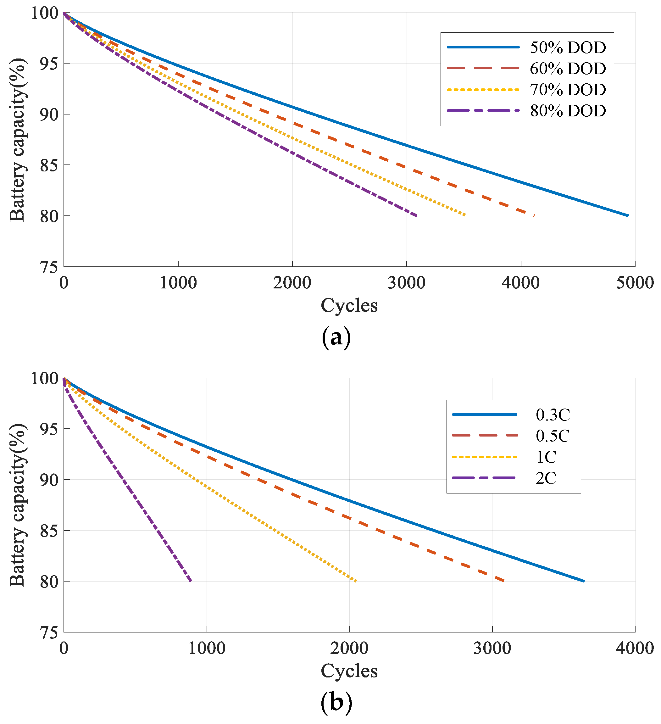
2.2.1. Battery Performance Degradation Model

The capacity degradation of batteries is defined as a percentage that equals the capacity loss divided by the nominal capacity after a period of operation. Normally, the batteries need to be replaced when the value exceeds 20%. Over the past few years, researchers focus on studying the performance degradation of the batteries as they often need to perform frequent charge and discharge operations. There have been considerable efforts to build models from different aspects, such as parasitic side reactions, solid-electrolyte interphase formation, resistance increase, etc., which lead to a capacity loss in battery [36,37]. Wang et al. [38] presented a semi-empirical life model based on the equation described by Bloom et al. [39], including three parameters (Ah-throughput, temperature, and discharge rate) shown in Equation (1) based on a large cycle test matrix:

$$Q_{\mathrm{loss}}=B\cdot \exp [\frac{-31,700+370.3\cdot \mathit{\text{C\_Rate}}}{R\cdot T_{\mathrm{en}}}]{\left(A_{\mathrm{h}}\right)}^{0.55},$$

(1)

where Q_loss is the percentage of capacity loss, B is the pre-exponential factor, R is the gas constant, T_en is the absolute temperature in K, A_h is the Ah-throughput, which is dependent on the cycle number, DOD, and full cell capacity and can be expressed as A_h = (cycle number) × (DOD) × (full cell capacity), and C_Rate is the discharge rate.

Based on this model, Masih-Tehrani et al. [11] built a battery life model to calculate the initial cost and 10-year replacement cost. Song et al. [12] performed a battery degradation experiment on the LiFePO₄ cell (3.3 V and 60 Ah) to calibrate the parameters indicated in Equation (2) and to verify the model accuracy:

$$Q_{\mathrm{loss}}=0.0032\cdot e^{-\left(\frac{15,162-1,516\cdot \mathit{\text{C\_Rate}}}{R\cdot T_{\mathrm{en}}}\right)}{\left(A_{\mathrm{h}}\right)}^{0.824},$$

(2)

To further explore the relationship between the battery capacity and cycle number at different DOD and C-rate, battery performance degradation model in Equation (2) is employed and the results in Figure 2 are obtained based on the MATLAB/Simulink model by setting the temperature as 303.15 K. It can be noted in Figure 2a that with the increase of the DOD from 50% to 80%, the cycles would be decreased from 5000 to 3000 with a C-rate of C/2 (30A). The similar tendency is that battery operating at a lower C-rate will achieve longer cycles demonstrated in Figure 2b from 0.3C to 2C (80% DOD). Through simulation results, it can be clearly seen that DOD and C-rate have a great influence on the battery capacity degradation. Therefore, it is essential to consider the impact of DOD within the battery degradation model when quantitatively evaluating the capacity loss during the HESS optimization.

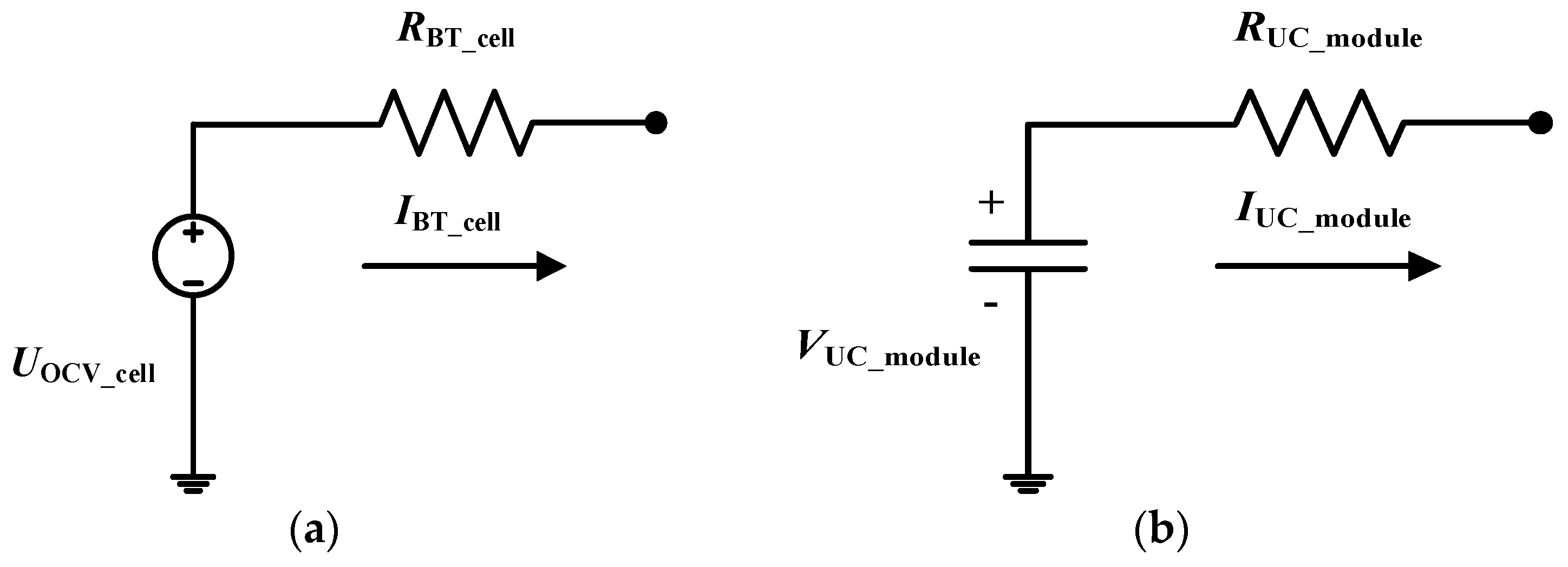
2.2.2. Battery Equivalent Circuit Model

Equivalent circuit models have been widely studied since they have relatively few parameters derived from empirical experience and experimental data and can be able to describe the dynamic characteristics of the battery with decent accuracy. These models normally use electrical components (resistances and capacitors) to depict the process of charging and discharging. As the simplest yet most effective equivalent circuit model, the Rint model [40], shown in Figure 3a, is adopted to represent the battery behavior.

The current can be calculated as follows:

$$I_{\mathit{\text{BT\_cell}}}=\frac{U_{\mathrm{OCV}\_\mathrm{cell}}-{(U_{\mathrm{OCV}\_\mathrm{cell}}^2-4\cdot R_{\mathrm{BT}\_\mathrm{cell}}\cdot P_{\mathrm{BT}\_\mathrm{cell}})}^{1/2}}{2\cdot R_{\mathrm{BT}\_\mathrm{cell}}},$$

(3)

where $U_{\mathrm{OCV}\_\mathrm{cell}}$, $P_{\mathrm{BT}\_\mathrm{cell}}$, and $R_{\mathrm{BT}\_\mathrm{cell}}$ are the open circuit voltage, the power, and the internal resistance of the battery cell, respectively.

The state of charge ($SoC$) at the discrete step k ($So{C}_{\mathrm{BT}\_\mathrm{cell}}(k)$) is defined as the current capacity ($Q(k)$) divided by the nominal capacity of the battery cell ($Q_{\mathrm{BT}\_\mathrm{cell}}$):

$$So{C}_{\mathrm{BT}\_\mathrm{cell}}(k)=Q(k)/Q_{\mathrm{BT}\_\mathrm{cell}}\cdot 100\%,$$

(4)

With a timestep of $\Delta t$, the $SoC$ at the next step is as follows:

$$So{C}_{\mathrm{BT}\_\mathrm{cell}}(k+1)=So{C}_{\mathrm{BT}\_\mathrm{cell}}(k)-(I_{\mathrm{BT}\_\mathrm{cell}}(k)\cdot \Delta t/Q_{\mathrm{BT}\_\mathrm{cell}})\cdot 100\%,$$

(5)

In terms of the battery pack, assume that the pack is formed via $N_{\mathrm{BT}}$ series and $M_{\mathrm{BT}}$ parallel battery cells [12]:

$$Q_{\mathrm{BT}}=M_{\mathrm{BT}}\cdot Q_{\mathrm{BT}\_\mathrm{cell}},$$

(6)

$$R_{\mathrm{BT}}=N_{\mathrm{BT}}\cdot R_{\mathrm{BT}\_\mathrm{cell}}/M_{\mathrm{BT}},$$

(7)

$$V_{\mathrm{BT}}=N_{\mathrm{BT}}\cdot V_{\mathrm{BT}\_\mathrm{cell}},$$

(8)

where $V_{\mathrm{BT}\_\mathrm{cell}}$ represents the voltage of the battery cell, and $Q_{\mathrm{BT}}$, $R_{\mathrm{BT}}$, and $V_{\mathrm{BT}}$ are the nominal capacity, the internal resistance, and the voltage of the battery pack, respectively.

2.2.3. UC Equivalent Circuit Model

With an increasing use of UCs in different applications, their modeling is indispensable for system design, condition monitoring, and performance evaluation. In the literature, numerous UC models have been reported, which can be mainly divided into empirical models and equivalent circuit models. As with the previous battery modeling method, the UC model is shown in Figure 3b.

Suppose that the pack is composed of the UC modules via $N_{\mathrm{UC}}$ series and $M_{\mathrm{UC}}$ parallel [12]:

$$C_{\mathrm{UC}}=M_{\mathrm{UC}}\cdot C_{\mathrm{UC}\_\mathrm{module}}/N_{\mathrm{UC}},$$

(9)

$$R_{\mathrm{UC}}=N_{\mathrm{UC}}\cdot R_{\mathrm{UC}\_\mathrm{module}}/M_{\mathrm{UC}},$$

(10)

$$V_{\mathrm{UC}}=V_{\mathrm{UC}\_\mathrm{module}}\cdot N_{\mathrm{UC}},$$

(11)

where $C_{\mathrm{UC}\_\mathrm{module}}$, $R_{\mathrm{UC}\_\mathrm{module}}$, and $V_{\mathrm{UC}\_\mathrm{module}}$ denote the nominal capacity, the internal resistance, and the voltage of the UC module, while $C_{\mathrm{UC}}$, $R_{\mathrm{UC}}$, and $V_{\mathrm{UC}}$ denote the same meanings of the UC pack.

The relationship between $So{C}_{\mathrm{UC}}$, $V_{\mathrm{UC}}$, and stored energy ($E_{\mathrm{UC}}$) of the UC pack can be deduced in Equations (12) and (13):

$$So{C}_{\mathrm{UC}}=V_{\mathrm{UC}}/V_{\mathrm{UC}\_\max },$$

(12)

$$E_{\mathrm{UC}}=0.5\cdot C_{\mathrm{UC}}\cdot V_{\mathrm{UC}\_\max }^2\cdot (1-So{C}_{\mathrm{UC}\_\min }^2),$$

(13)

where $V_{\mathrm{UC}\_\max }$ and $V_{\mathrm{UC}\_\min }$ are the UC pack voltage in a fully charged condition and the lower limit of the UC pack $SoC$. Due to the simplified UC model used in this paper, the variation of $C_{\mathrm{UC}}$ with $V_{\mathrm{UC}}$ has not been considered. It can be inferred from Equation (13) that UC pack can release 75% of its stored energy when the $So{C}_{\mathrm{UC}}$ drops from 100% to 50%. Therefore, the $So{C}_{\mathrm{UC}\_\min }$ is generally set more than 50% from the efficiency perspective. Given the fact that UCs have long cycle times (more than 500,000 cycles), their capacity loss will not be considered in the model.

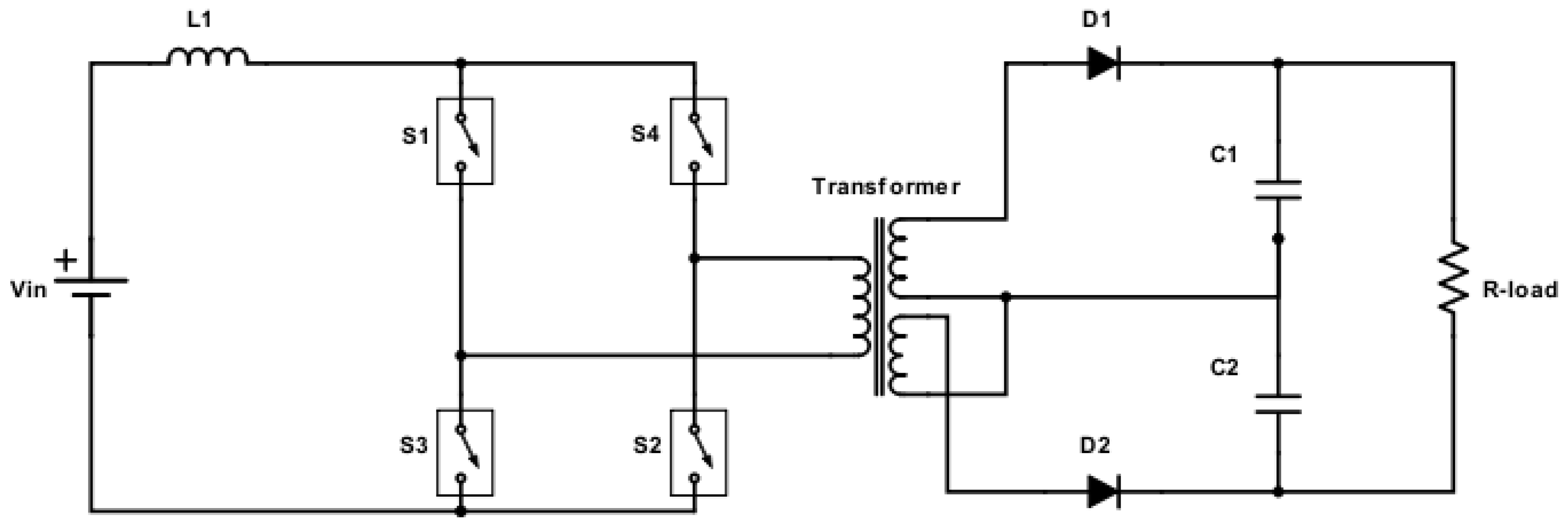
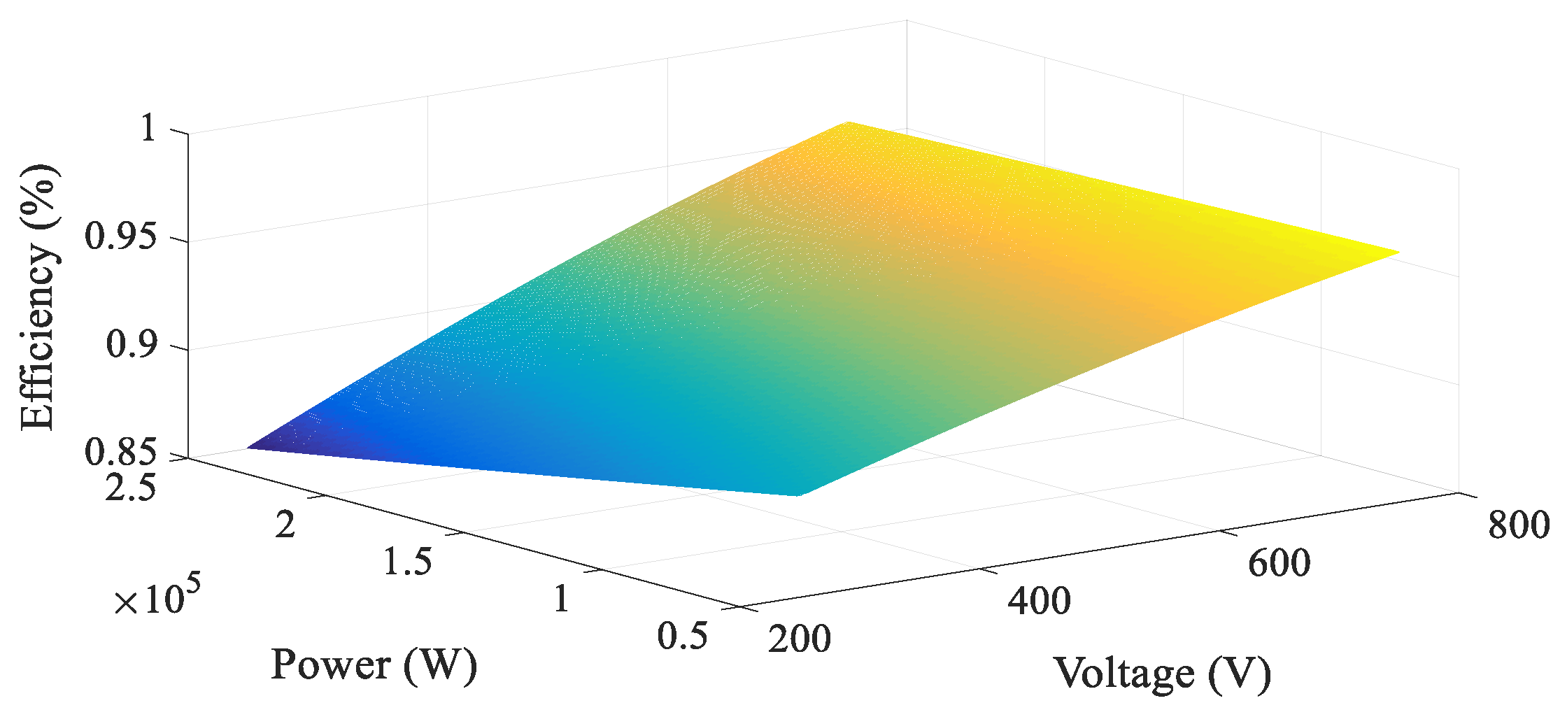
2.2.4. DC/DC Converter Power Loss Model

As the connection between the UC and the DC bus, the DC/DC converter can not only regulate the voltage but control the power supply of the UC. In order to increase the accuracy of the simulation process, a voltage doubler boost converter introduced in [41] is simulated in MATLAB/Simulink to develop a power loss model. This converter circuit diagram is displayed in Figure 4.

The five main losses in converter including switch turn on loss, switch turn off loss, switch conduction loss, diode conduction loss, and diode recovery loss. The switch losses can be calculated by collecting the fall and rise time of the switch from data sheet. We assume switch voltage and current have a linear behavior shown in Figure 5.

Therefore, the losses can be calculated as follows:

$$P_{\mathrm{switching}\mathrm{loss}}=P_{t_{\mathrm{r}}}+P_{t_{\mathrm{f}}}=(\frac{1}{6}\cdot V_{\mathrm{m}}\cdot I_{\mathrm{m}}\cdot (t_{\mathrm{r}}+t_{\mathrm{f}})\cdot f)\cdot n_{\mathrm{s}},$$

(14)

$$P_{\mathrm{switch}\mathrm{cond}}=R_{\mathrm{dsON}}\cdot I_{\mathrm{T}\left(\mathrm{rms}\right)}^2\cdot n_{\mathrm{s}},$$

(15)

$$P_{\mathrm{diode}\mathrm{loss}}=(V_{\mathrm{F}}\cdot I_{\mathrm{F}\left(\mathrm{AV}\right)}+R_{\mathrm{F}}\cdot I_{\mathrm{F}\left(\mathrm{rms}\right)}^2)\cdot n_{\mathrm{d}},$$

(16)

where t_r and t_f are the rise and fall time available on the data sheet, V_m and I_m are the maximum voltage and current across the switch, f is the frequency of the switch, n_s and n_d represent the number of switches and diodes, R_dsON is the transistor resistance, I_T(rms) and I_F(rms) are the RMS current of each switch and diode, which are computed over the overall sampling time period by assuming these currents equal to zero outside the conduction period, V_F is the diode forward voltage, I_F(AV) is the diode average current, and R_F is the diode resistance.

In addition, a high frequency transformer shown in Figure 4 is used between the switches and capacitors for isolation and voltage translation requirements. The main transformer losses consist of copper losses, eddy current losses and hysteresis loss in the core of the transformer. In this work, it is assumed that the total transformer loss is 1% of the net output power. Moreover, power losses in inductor and capacitors are ignored and ideal components are considered. When the voltage across the diode is negative and diode is in reverse-bias mode, it is assumed that the diode is open circuit and no power loss during this mode is considered.

3. Nested Optimization of HESS

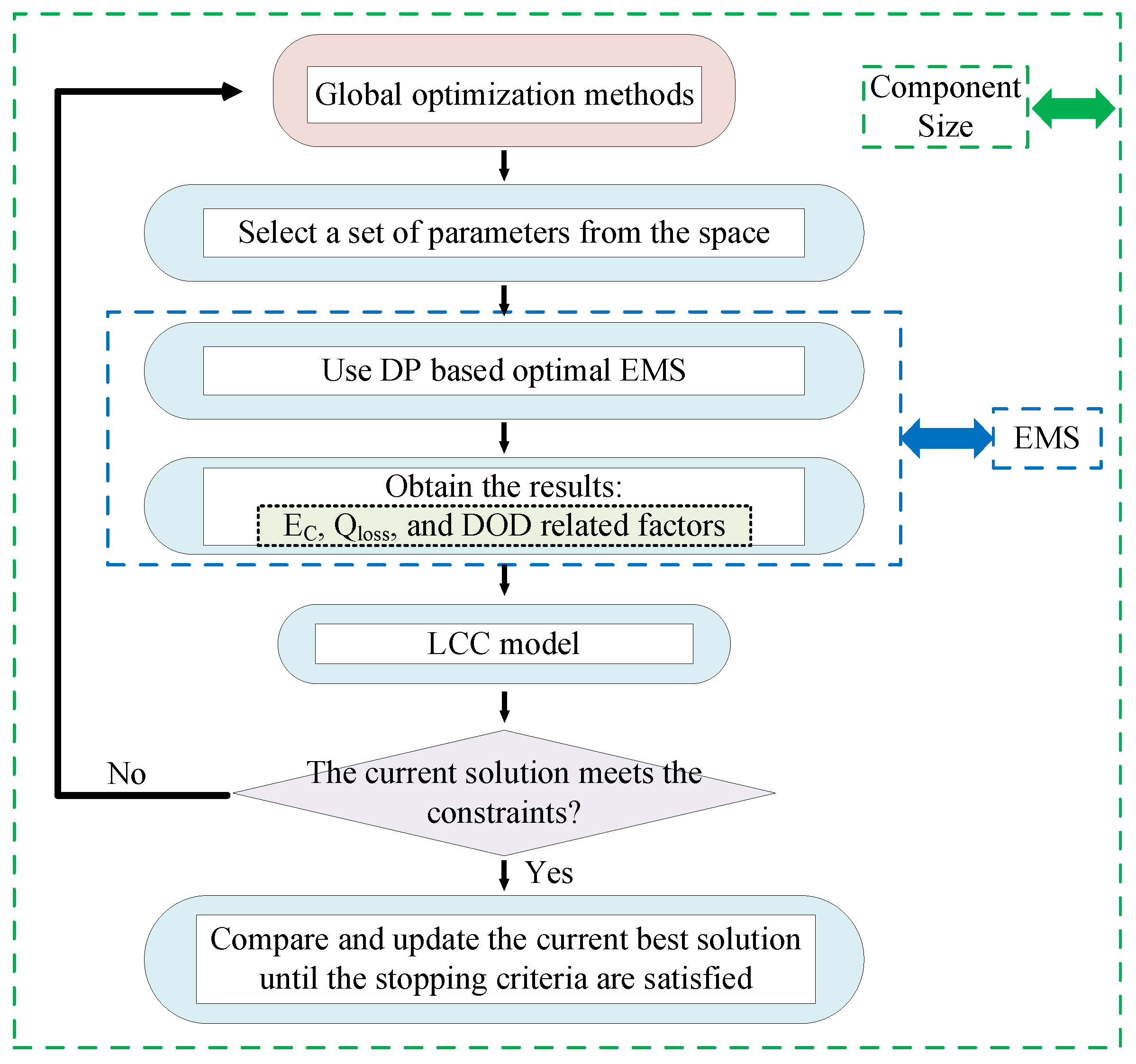
3.1. Problem Formulation

The performance of the HESS is affected by three aspects: driving cycle, component size, and EMS. Accordingly, a nested, dual-level optimization framework can be formulated in Figure 6 based on given driving cycles to minimize the life-cycle cost of HESS.

DP-based optimal EMS is nested within component size to obtain the minimum energy consumption (E_C), i.e., every evaluation of a component size requires the optimization of the EMS. HESS component size (N_BT, M_BT, N_UC, and M_UC) and battery DOD (DOD_BT) are acted as optimization variables dependent on the DC bus voltage as well as the maximal output current of HESS, and the performance requirements are employed as constraints.

Initially, the ranges of optimization variables need to be defined as the design space. Then, global optimization methods will be used to find the optimal solution within the design space and the key steps of the nested optimization are as follows:

(1)

Select a set of parameters as the input from the design space based on the search method of the optimization algorithm.

(2)

DP-based optimal EMS is used to evaluate the corresponding E_C, Q_loss, and DOD-related factors.

(3)

The results obtained by DP are utilized to achieve the objective function via the LCC model.

(4)

If the current solution meets the constraints, compare and update the best solution and then terminate until the stopping criteria are satisfied. Otherwise, repeat the steps (1) to (3) until the global stopping conditions are met.

3.2. DP-Based EMS

The DP is widely applied to solve the problem of EMS for HESS-based vehicles [42,43,44]. In this paper, the DP implemented by Song et al. [44] is employed aiming at minimizing the E_C of the given power profiles, with an objective function and constraints listed as follows:

$$\min E_{\mathrm{C}}={\displaystyle \sum _{k=1}^T\left[\Delta E_{\mathrm{BT}}(k)+\Delta E_{\mathrm{UC}}(k)\right]},$$

(17)

$$s.t.\{\begin{array}{l}{P}_{\mathrm{dem}}(k)=P_{\mathrm{cycle}}(k),k\in [1,T]\\ So{C}_{\mathrm{UC}}\in [So{C}_{\mathrm{UC}\_\mathrm{L}},So{C}_{\mathrm{UC}\_\mathrm{H}}]\\ So{C}_{\mathrm{UC}\_0}=So{C}_{\mathrm{UC}\_\mathrm{end}}\\ I_{\mathrm{BT}}\in [0,I_{\mathrm{BT}\_\max }]\\ P_{\mathrm{UC}}\in [P_{\mathrm{UC}\_\min },P_{\mathrm{UC}\_\max }]\end{array},$$

(18)

where $\Delta E_{\mathrm{BT}}$ and $\Delta E_{\mathrm{UC}}$ are the energy consumption of the battery pack of UC pack, respectively, $P_{\mathrm{dem}}$ is the power demand, $P_{\mathrm{cycle}}$ is the total power of the driving cycle, $So{C}_{\mathrm{UC}\_\mathrm{L}}$ and $So{C}_{\mathrm{UC}\_\mathrm{H}}$ are the lower and upper limits of the $So{C}_{\mathrm{UC}}$, $So{C}_{\mathrm{UC}\_0}$ is the initial $So{C}_{\mathrm{UC}}$ value, $So{C}_{\mathrm{UC}\_\mathrm{end}}$ is the end $So{C}_{\mathrm{UC}}$ value, $P_{\mathrm{UC}\_\min }$ and $P_{\mathrm{UC}\_\max }$ are the minimal and maximal power of the UC pack, and $I_{\mathrm{BT}\_\max }$ is the maximal discharge current of the battery pack.

The power of the battery and UC needs to satisfy the power demand shown in Equation (19), where $P_{\mathrm{BT}}$ and $P_{\mathrm{UC}}$ represent the actual output power of the battery and UC packs after considering the efficiency of the DC/DC converter:

$$P_{\mathrm{dem}}(k)=P_{\mathrm{BT}}(k)+P_{\mathrm{UC}}(k),$$

(19)

UC voltage $V_{\mathrm{UC}}$ and voltage change $\Delta V_{\mathrm{UC}}$ are regarded as the state and decision variables of DP, respectively. $\Delta V_{\mathrm{UC}}(k,k-1)$ in Equation (20) represents the voltage change of UC from k − 1 step to k step. Besides, the energy consumption of UC and battery can be calculated via Equations (21) and (22):

$$V_{\mathrm{UC}}(k)=V_{\mathrm{UC}}(k-1)+\Delta V_{\mathrm{UC}}(k,k-1),$$

(20)

$$\Delta E_{\mathrm{UC}}(k)=0.5\cdot C_{\mathrm{UC}}\cdot (V_{\mathrm{UC}}^2(k)-V_{\mathrm{UC}}^2(k-1)),$$

(21)

$$\Delta E_{\mathrm{BT}}(k)=\left|P_{\mathrm{BT}}(k)\right|\cdot \Delta t(k),$$

(22)

3.3. LCC Model

The LCC model is established including the capital cost, operating cost, and replacement cost. These costs can be calculated based on the following equations:

$$Cos{t}_{\mathrm{cap}}=(B{T}_{\mathrm{cap}}+U{C}_{\mathrm{cap}}+D{C}_{\mathrm{cap}})\cdot CRF,$$

(23)

$$CRF=\frac{i\cdot {(1+i)}^{RT}}{{(1+i)}^{RT}-1},$$

(24)

$$B{T}_{\mathrm{cap}}=C_{\mathrm{kWh}\_\mathrm{BT}}\cdot N_{\mathrm{BT}}\cdot M_{\mathrm{BT}}\cdot E_{\mathrm{BT}\_\mathrm{cell}},$$

(25)

$$U{C}_{\mathrm{cap}}=C_{\mathrm{kWh}\_\mathrm{UC}}\cdot N_{\mathrm{UC}}\cdot M_{\mathrm{UC}}\cdot E_{\mathrm{UC}\_\mathrm{cell}},$$

(26)

$$D{C}_{\mathrm{cap}}=C_{\mathrm{kW}\_\mathrm{DC}}\cdot (P_{\mathrm{acc}}+P_{\mathrm{UC}\_\max }),$$

(27)

In terms of the operating cost and replacement cost, Equations (28)–(31) are listed as follows:

$$Cos{t}_{\mathrm{ope}}=(\Delta E_{\mathrm{BT}}+\Delta E_{\mathrm{UC}})\cdot C_{\mathrm{kWh}\_\mathrm{e}}/T\cdot T_{\mathrm{op}}\cdot U,$$

(28)

$$Q_{\mathrm{loss}\_\mathrm{y}}=Q_{\mathrm{loss}}/T\cdot T_{\mathrm{op}}\cdot U\cdot 360\cdot RT,$$

(29)

$$\mathit{\text{n\_BT}}=ceil(Q_{\mathrm{loss}\_\mathrm{y}}/0.2-1),$$

(30)

$$Cos{t}_{\mathrm{rep}}={\displaystyle \sum _{n=1}^{n\_BT}{(1+i)}^{-n\cdot 0.2}\cdot B{T}_{\mathrm{cap}}\cdot CRF},$$

(31)

All the variables mentioned in Equations (23)–(31) have listed in

Table 1. Variables in the LCC model.

Variable	Definition	Unit
Costcap	Capital costs of battery, UC, and DC/DC converters	€/year
BTcap	Capital cost of battery	€
UCcap	Capital cost of UC	€
DCcap	Capital costs of battery, UC, and DC/DC converters	€
CRF [45]	capital recovery factor	1/year
i	interest rate	%
RT	reference time	years
CkWh_BT	referential cost of battery	€/kWh
CkWh_UC	referential cost of UC	€/kWh
CkW_DC	referential cost of DC/DC converters	€/kW
Costope	operating cost of electricity	€/day
CkWh_e	referential cost of electricity	€/kWh
T	number of sample points for the driving cycle	/
Top	Vehicles operating time	hours/day
U	mean utilization of vehicles	%
Qloss_y	battery capacity loss within the reference time	%
n_BT	number of battery replacements during the reference time	/
Costrep	replacement cost of the battery	€/year

to improve the readability. In addition, we assume that vehicles can operate 360 days a year and batteries need to be replaced when the loss exceeds 20%. $ceil()$ is the function obtaining the higher integer of its argument to calculate the $\mathit{\text{n\_BT}}$.

4. Global Optimization Algorithms

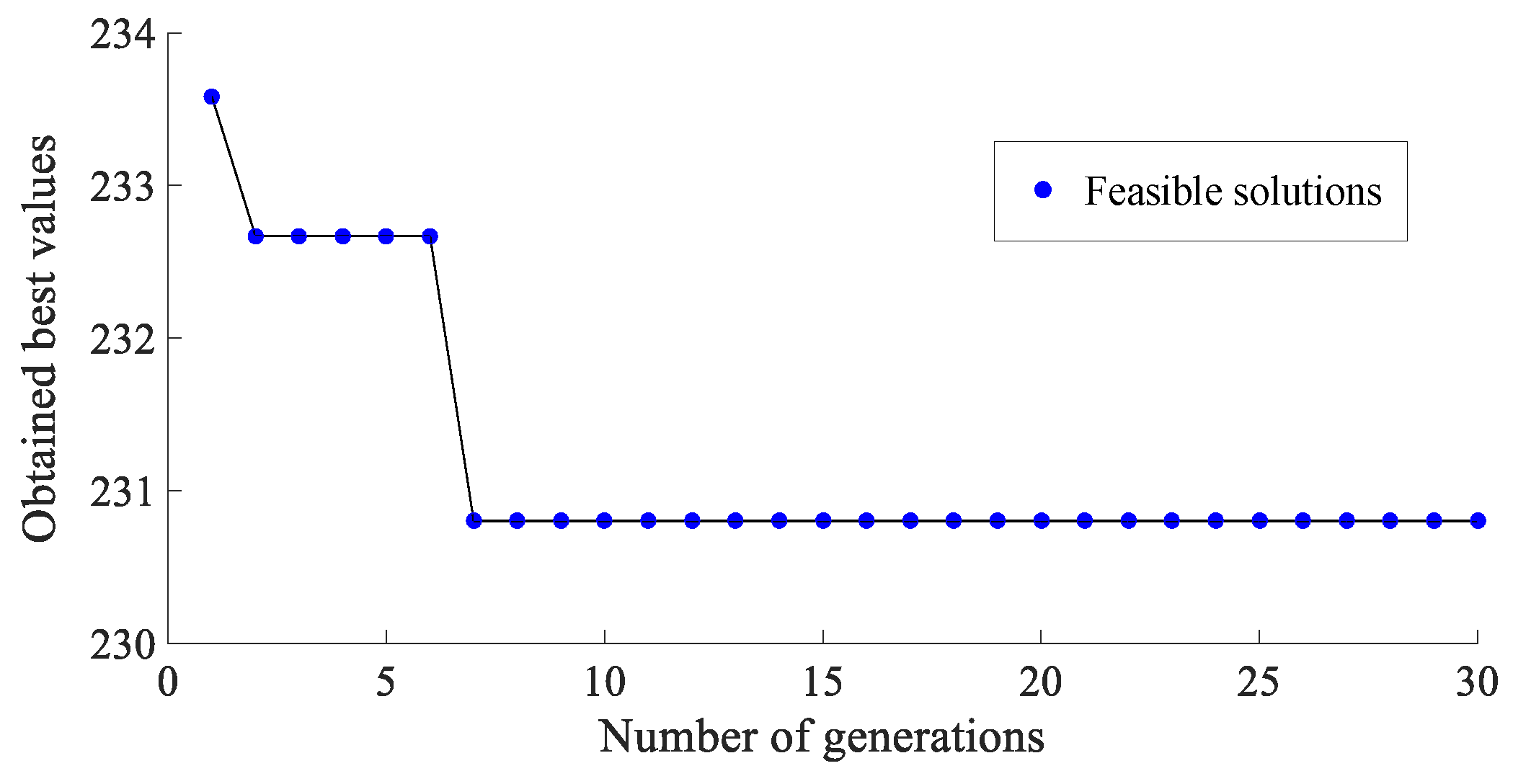
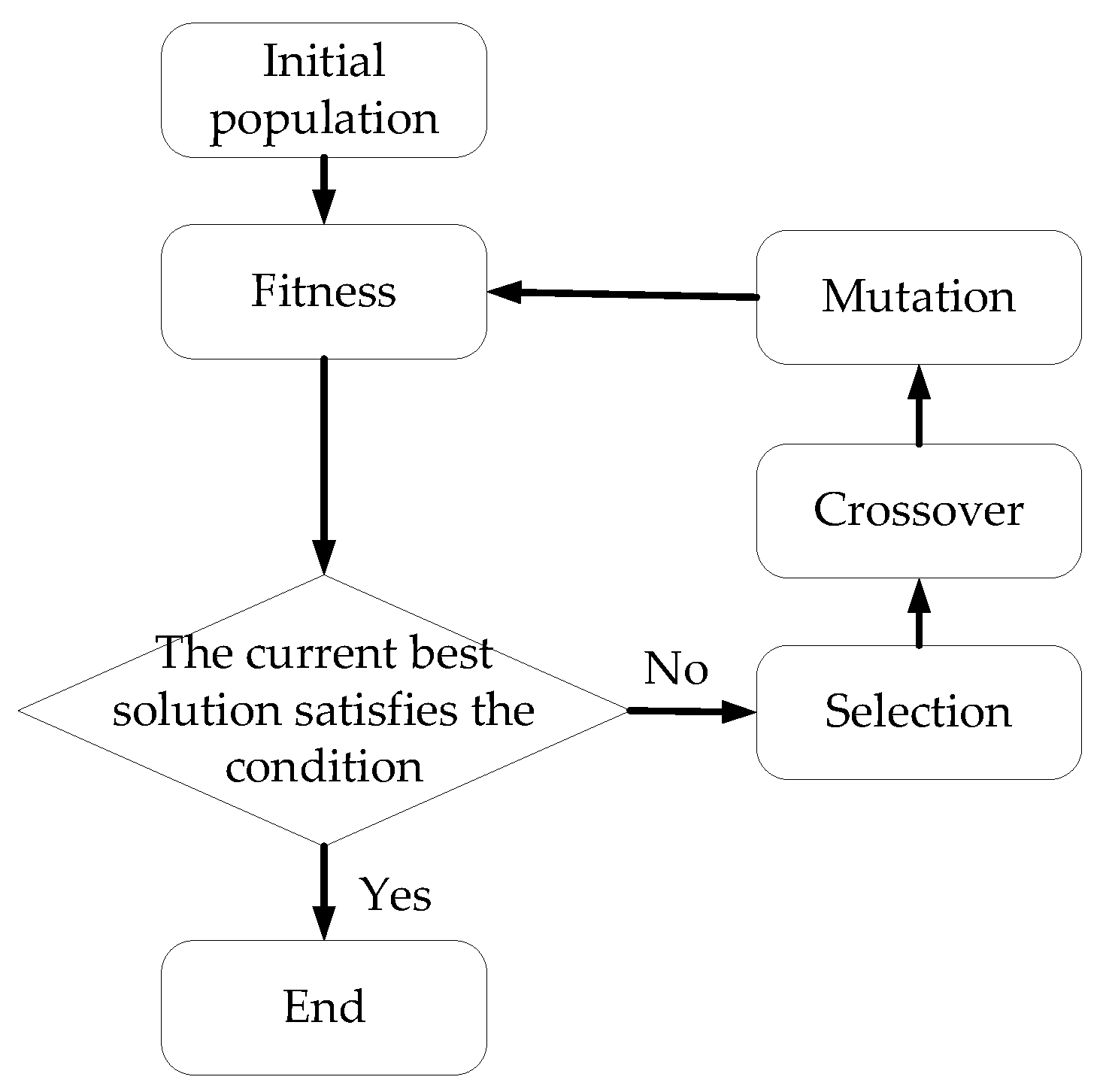
In order to solve this complex and challenging optimization problem, global optimization algorithms such as GA and MSSR are introduced respectively to attain the best solution.

4.1. GA

The basic principles of GA were first formulated by Holland [29]. As a classical optimization method, GA is inspired by the mechanism of natural selection, a biological process in which stronger individuals are likely to be the winners in a competing environment [46]. It operates on a population of individuals (potential solutions), each of which is an encoded string (chromosome), containing the decision variables (genes) [47].

The structure of GA is composed by an iterative procedure with the following five main steps and the flowchart is shown in Figure A1 in the Appendix A:

(1)

Produce an initial population.

(2)

Evaluate the fitness function of each individual of the population.

(3)

Select individuals from the current population to be parents.

(4)

Generate the next population via crossover and mutation.

(5)

Iterate steps (2) to (4) until the stopping criteria are fulfilled.

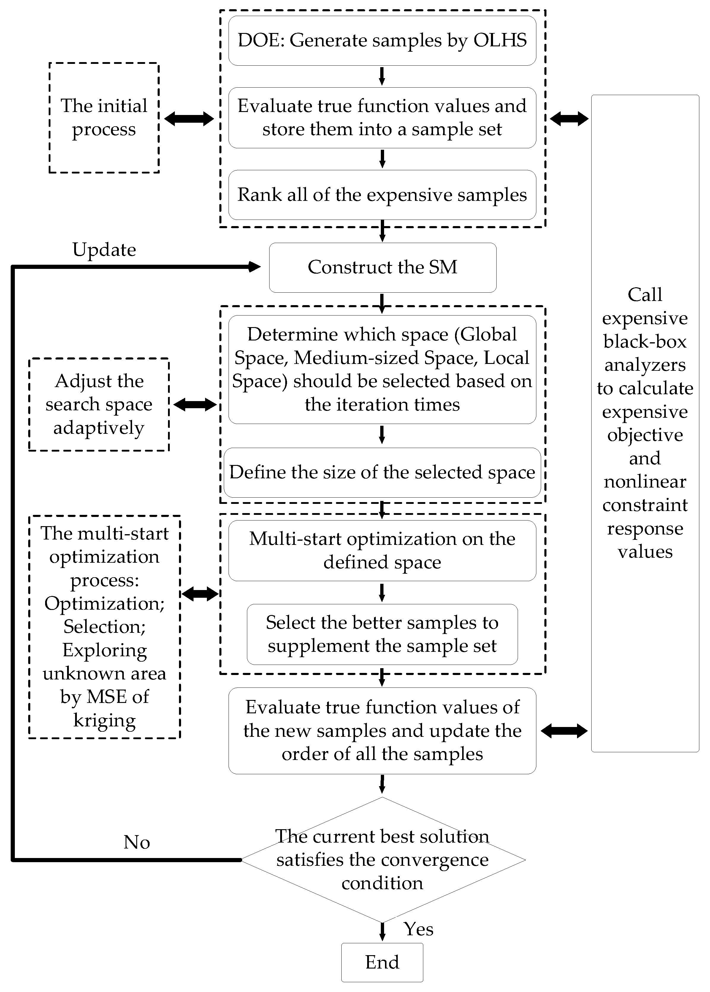
4.2. MSSR

As a more efficient SBGO approach, MSSR uses a kriging-based surrogate model (SM), a multi-start scheme, and alternating sampling over the global space (GS), the reduced medium space (MS), and the local space (LS) to carry out the global optimization search. The flowchart of MSSR is illustrated in Figure A2 in the Appendix A.

The complete MSSR global optimization can be divided into two parts, the initial process (steps (1) to (3)) and the search loop (steps (4) to (10)), which are listed as follows [32]:

(1)

Design of experiment: using optimized Latin hypercube sampling to generate sample points in the entire design space.

(2)

Evaluate the expensive function with these sample points and store the results in the sample set.

(3)

Rank all expensive samples based on their function values (add a large penalty factor of 10⁶ to the value if the point does not meet the constraints).

(4)

Build the kriging-based SM.

(5)

Determine which space should be explored based on the present number of iterations. The global search, medium-sized search, and local search will be implemented in the process.

(6)

Define the size of the search space according to the expensive sample set.

(7)

Utilize the multi-start local optimization method to optimize the kriging-based SM in the defined space.

(8)

Store the local optimal solutions obtained from the database “potential sample points” and select better samples. If there is no better sample, two new samples from the unknown area will be selected.

(9)

Evaluate the expensive function with the selected sample points and update the order of the expensive samples in step (3).

(10)

Terminate the loop if the current best sample value satisfies the stopping criteria. Otherwise, update the SM and repeat the steps (4) to (9) until the stopping criteria are satisfied.

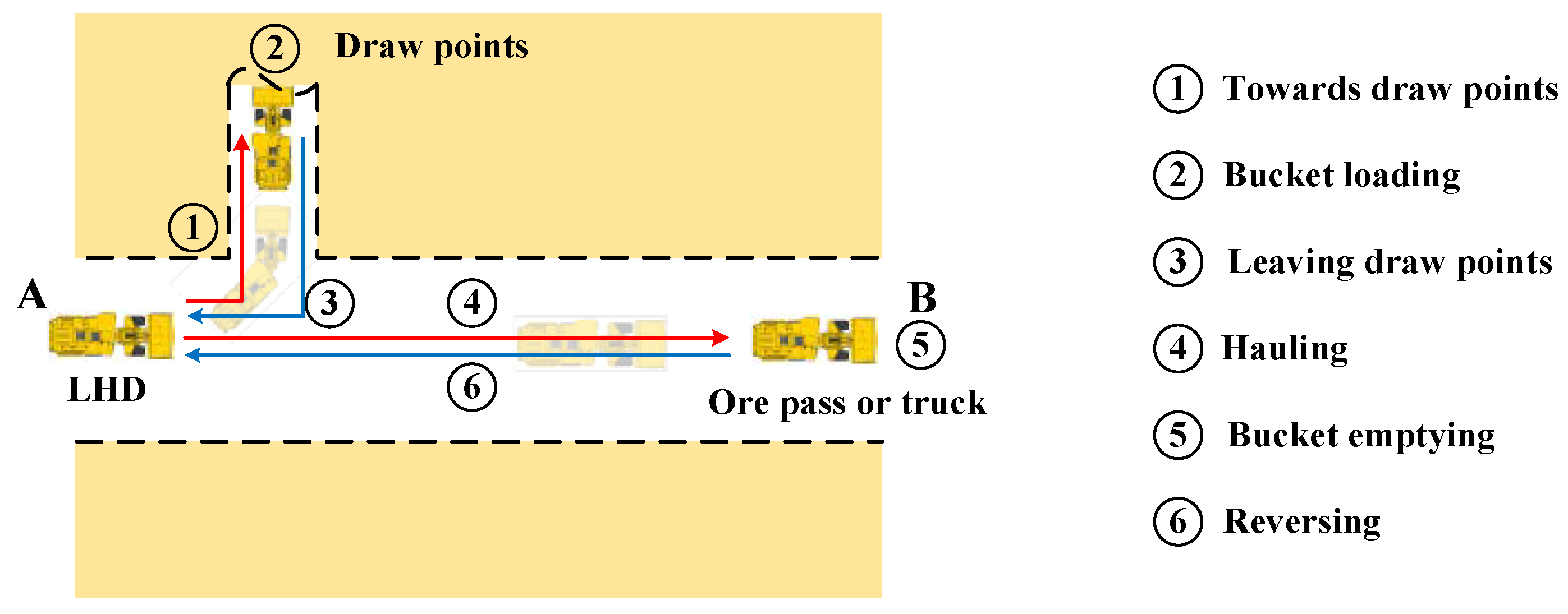
5. Dynamic On-Off Power Loads Example: LHD

As a dynamic on-off power loads application, LHD will be used in this paper as an example to verify the proposed HESS design optimization method. LHDs are one of the most commonly used equipment in the mining industry and are employed to load the ore at the draw points or in the stopes and to haul it to the ore passes or the mining trucks. Due to the dramatic and frequent power variations, a HESS-based LHD is presented to improve the efficiency and extend the battery life.

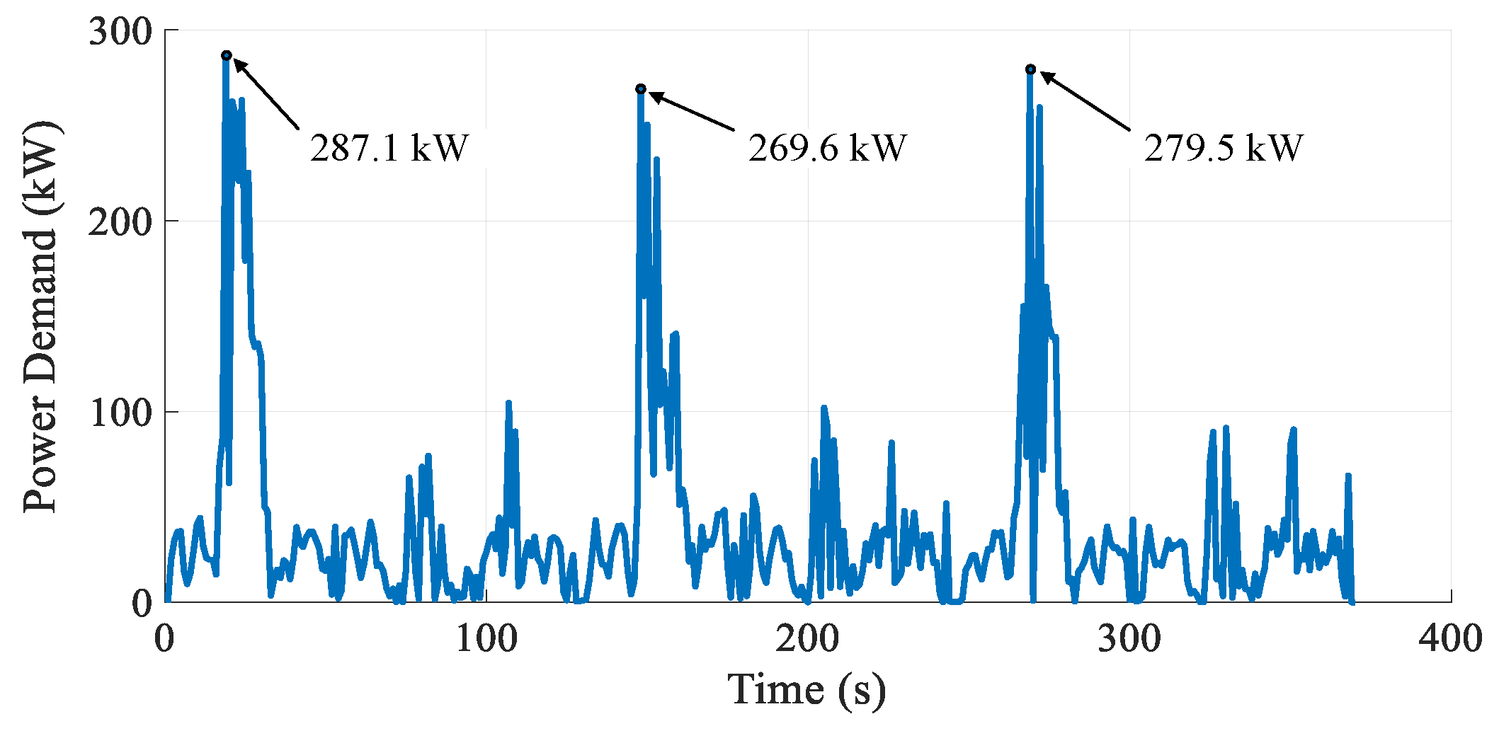
5.1. LHD Data Description

Figure 7 illustrates a driving cycle of LHDs, which can be divided into six phases: towards draw points, bucket loading, leaving draw points, hauling, bucket emptying, and reversing. The power demand shown in Figure 8 was collected from the underground mine field tests of a 14-ton diesel-electric LHD, where the duration is 370 s, the sampling frequency is 1 s, and the peak power is 287.1 kW. Figure 8 includes three complete driving cycles, the maximum power of each bucket loading phase is 287.1, 269.6 and 279.5 kW, respectively. It can be seen that the power demand is high during the bucket loading phase, while relatively low in other phases.

The key parameters of the battery cell and UC module are listed in

Table 2. Key parameters of the battery cell and UC module.

Battery Cell		UC Module
Nominal voltage (V)	3.3	Nominal voltage (V)	48
Nominal capacity (Ah)	60	Nominal capacity (F)	165
Stored energy (kWh)	0.198	Stored energy (kWh)	0.053
Internal resistance (mΩ)	1.5	Internal resistance (mΩ)	6.3

, which are provided by the manufacturers (China Aviation Lithium Battery, Luoyang, China and Maxwell, San Diego, CA, USA). For the DC/DC power loss model, a 3D efficiency map illustrated in Figure 9 can be generated by changing the input voltage varied from 250 V to 750 V and load power between 50 kW and 250 kW.

The objective function, i.e., the life-cycle cost of HESS, can be calculated by Equation (32). LHD’s working hours (W_hrs) is set as the constraint of the optimization not only because it is an important design index for the powertrain system but because it has the relationship with the variables and needs to be computed every time by DP algorithm, listed in Equation (33).

W_hrs equals the total capacity (Ah) of the battery pack divided by the demand capacity (Ah) that can be calculated from the output power of battery and accessories as well as DOD_BT. Optimization variables including HESS size and battery DOD are shown in Equation (34):

$$\min LCC=Cos{t}_{\mathrm{cap}}/360+Cos{t}_{\mathrm{ope}}+Cos{t}_{\mathrm{rep}}/360,$$

(32)

$$W_{\mathrm{hrs}}=Q_{\mathrm{BT}\_\mathrm{cell}}\cdot M_{\mathrm{BT}}/\left({\displaystyle \sum (((P_{\mathrm{BT}}+P_{\mathrm{acc}}/Ef{f}_{\mathrm{DC}})/V_{\mathrm{BT}}\cdot 1000)\cdot t/3600)}/DO{D}_{\mathrm{BT}}\right)\cdot T/3600,$$

(33)

$$\left\{\begin{array}{l}(N_{\mathrm{BT}},M_{\mathrm{BT}},N_{\mathrm{UC}},M_{\mathrm{UC}},DO{D}_{\mathrm{BT}})|N_{\mathrm{BT}}\in \left\{170,172,174,\cdots ,200\right\},\\ M_{\mathrm{BT}}\in \left\{6,7,8,9,10\right\},N_{\mathrm{UC}}\in \left\{11,12,13,14,15\right\},\\ M_{\mathrm{UC}}\in \left\{1,2\right\},DO{D}_{\mathrm{BT}}\in [50\%,80\%]\end{array}\right\},$$

(34)

where LCC is in €/day, P_BT is the battery power obtained by DP, P_acc is the nominal power of the accessories, Eff_DC is the efficiency of the low-voltage unidirectional DC/DC converter, which is set as 90% in this paper, t is the discrete time and normally equals to 1 s, and T is the number of sample points for the driving cycle.

As for the design space, DOD_BT from 50% to 80% is added as a new continuous variable compared to our work in [8]. N_BT belongs to an even number from 170 to 200 due to the working range of the DC bus (400 V–720 V) as well as for easy arrangement. M_BT ranges from 6 to 10 because of considering the constraint and the influence of DOD_BT. The numbers of N_UC and M_UC are dependent on the installation space and converter voltage and power.

All the parameters for the DP and LCC model are defined in

Table 3. Parameters for the DP algorithm and LCC model.

Name	Coefficient	Value	Unit
DP algorithm	$T$	370	s
	$So{C}_{\mathrm{UC}\_\mathrm{L}}$	50	%
	$So{C}_{\mathrm{UC}\_\mathrm{H}}$	100	%
	$So{C}_{\mathrm{UC}\_0}$($So{C}_{\mathrm{UC}\_\mathrm{end}}$)	100	%
	$P_{\mathrm{UC}\_\min }$	−250	kW
	$P_{\mathrm{UC}\_\max }$	250	kW
	$I_{\mathrm{BT}\_\max }$	0.5C	A
LCC model	$i$	2.5 [45]	%
	$RT$	10 [48]	Years
	$C_{\mathrm{kWh}\_\mathrm{BT}}$	500 [22]	€/kWh
	$C_{\mathrm{kWh}\_\mathrm{UC}}$	4000 [22]	€/kWh
	$C_{\mathrm{kW}\_\mathrm{DC}}$	150 [22]	€/kW
	$C_{\mathrm{kWh}\_\mathrm{e}}$	0.05 [45]	€/kWh
	$U$	60 [48]	%
	$T_{\mathrm{en}}$	303.15	K
	$P_{\mathrm{acc}}$	5	kW

. The interval of the UC voltage is 2 V. According to the operating characteristics of the LHDs, assume that they work 24 h per day and 360 days per year.

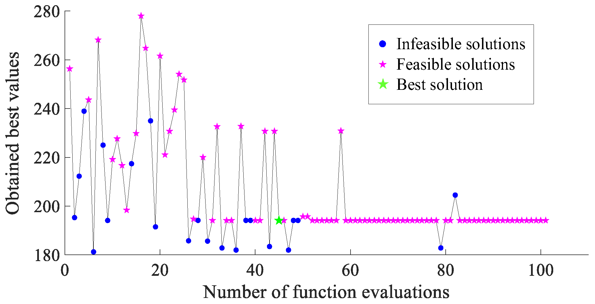
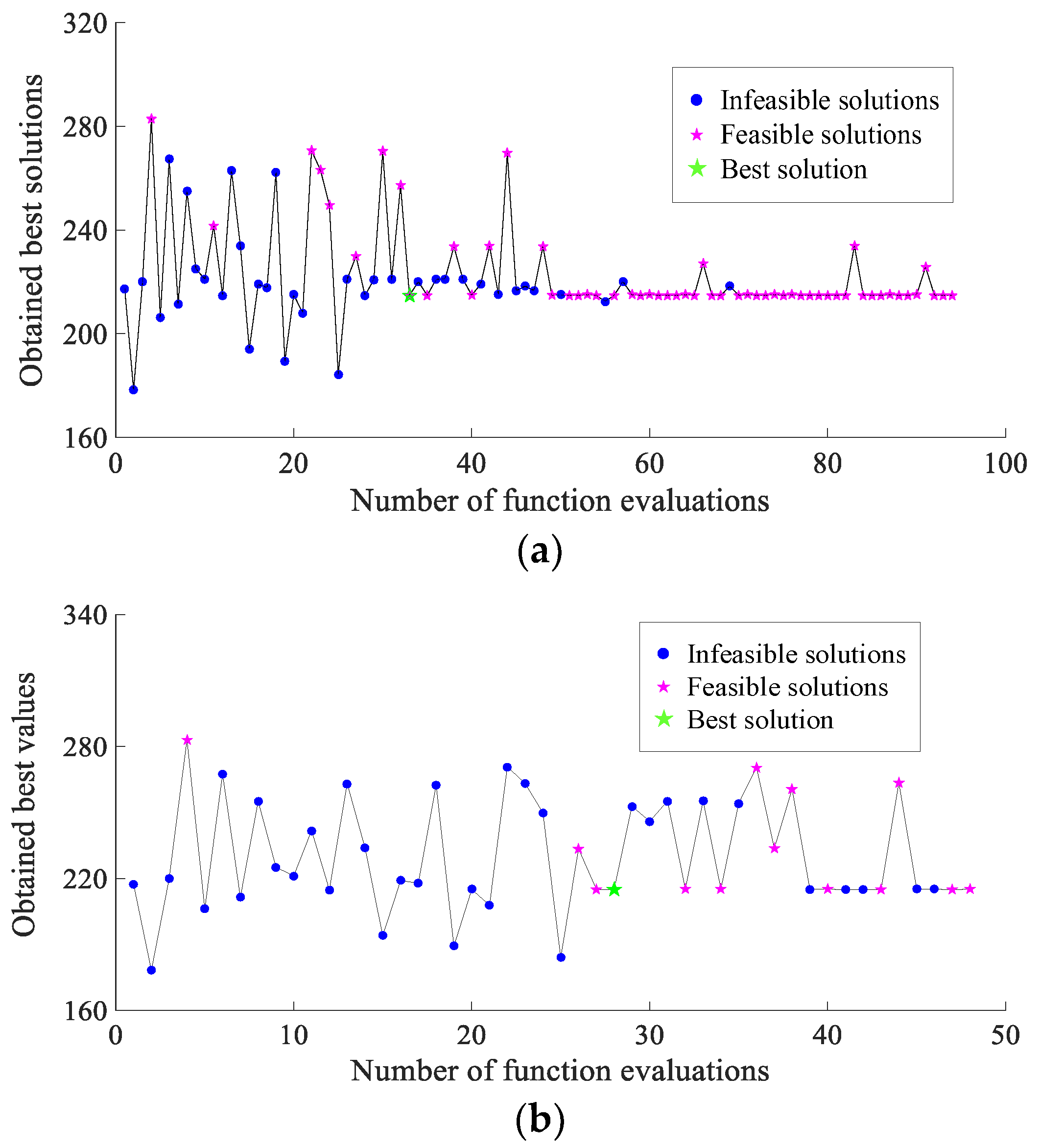
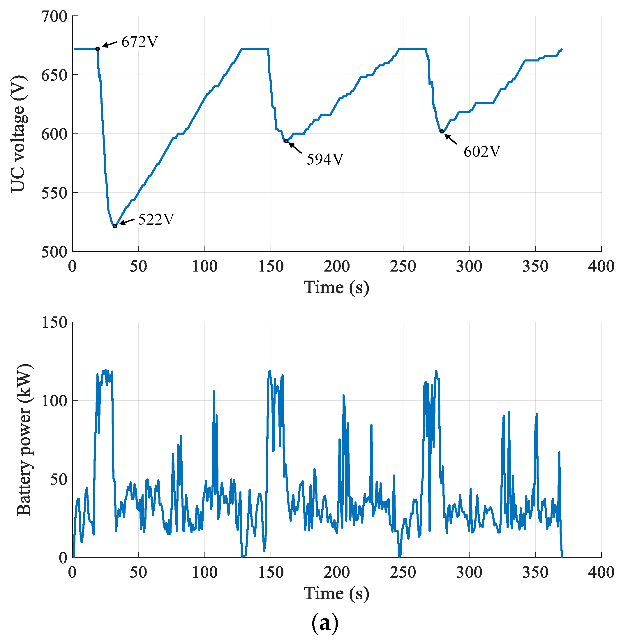
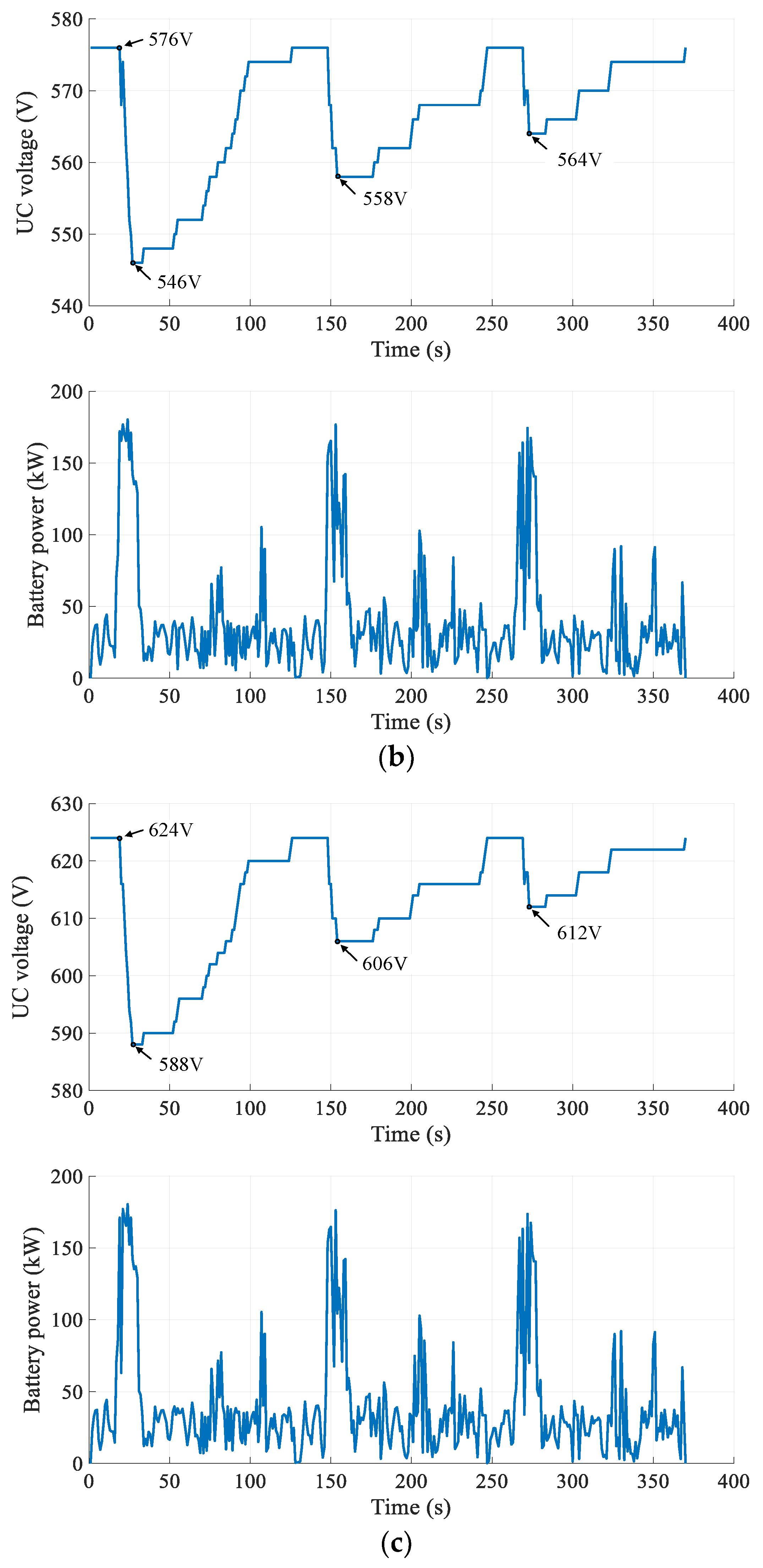
5.2. Optimization Results

To apply GA to solve this problem, the fitness function shown in Equation (32) is used to evaluate the status of each solution and the ranges of variables are also listed in Equation (34). However, as GA is not directly applicable to constrained optimization problems, the constraint illustrated in Equation (33) is handled by using penalty function. Besides, due to the fact that the first four variables are discrete and the other one is continuous, which belongs to a mixed integer problem, the first four variables need to be converted to integers before the DP algorithm.

According to the structure of the nested optimization framework shown in Figure 6, DP-based EMS and LCC model require to be evaluated for obtaining the fitness function of each individual. Using the GA MATLAB codes developed by our research team, only a few parameters including variable range (Equation (34)), population size, number of generations, crossover rate, and mutation rate need to be modified, which are exhibited in

Table 4. Parameters for the GA.

Coefficient	Value
Population size	10
Number of generations	30
Crossover rate	1.0
Mutation rate	0.01

.

Given that numerous battery LHD products, such as Atlas Copco’s Scooptram ST7 Battery and RDH Mining Equipment’s MUCKMASTER 300EB and 600EB, have an average operating time of 4 h, the constraint is set as $W_{\mathrm{hrs}}\ge 4$. After more than 126.23 h of computation, the best result is 230.81 €/day and the corresponding variables are $N_{\mathrm{BT}}=198$, $M_{\mathrm{BT}}=10$, $N_{\mathrm{UC}}=12$, $M_{\mathrm{UC}}=2$, and $DO{D}_{\mathrm{BT}}=0.5534$. Figure 10 displays the optimization process history of the problem. GA has been found to be able to converge to the optimum within 30 generations after several generations of function evaluations. Due to the fact that the optimization problem has changed to the unconstrained one, the solutions shown in Figure 10 are all feasible solutions. All the calculations in this paper are performed on a computer with Intel Xeon E5-2620 v3 CPU (2.40 GHz) and 32 GB RAM.

The nested optimization problem proposed in this paper is computationally expensive because it takes around 30 min to calculate the DP every time. Therefore, how to reduce the number of the expensive evaluation is crucial for a desirable optimization tool.

Using the same objective function, constraint, variables, and method of converting discrete variables to integers, the iterative results obtained by MSSR are presented in Figure 11 with 25 sample points and 50 iterations. The solutions can be divided into feasible and infeasible solutions according to whether the solution satisfies the constraint $W_{\mathrm{hrs}}$. The computation time is 49.13 h and the best result is 194.07 €/day achieved from the 45th evaluation. The variables of the best solution are $N_{\mathrm{BT}}=170$, $M_{\mathrm{BT}}=7$, $N_{\mathrm{UC}}=14$, $M_{\mathrm{UC}}=1$, and $DO{D}_{\mathrm{BT}}=0.7793$.

It can be seen from Figure 11 that after 25 sample points of training the number of infeasible solutions is decreasing; the optimal area can be found quickly with the increase of the number of function evaluations (NFE) and then a lot of searches nearby are conducted to compare the current results until satisfying the stopping criteria.

To comprehensively compare the performances between GA and MSSR, all the results are demonstrated in

Table 5. The results of GA and MSSR.

Algorithm	LCC (€/day)	Computation Time (h)	NFE	${\mathit{N}}_{\mathbf{B}\mathbf{T}}$	${\mathit{M}}_{\mathbf{B}\mathbf{T}}$	${\mathit{N}}_{\mathbf{U}\mathbf{C}}$	${\mathit{M}}_{\mathbf{U}\mathbf{C}}$	$\mathit{D}\mathit{O}{\mathit{D}}_{\mathbf{B}\mathbf{T}}$
GA	230.81	126.23	300	198	10	12	2	0.5534
MSSR	194.07	49.13	101	170	7	14	1	0.7793

. The LCC acquired by MSSR is 15.9% lower than that of GA; the computation time of MSSR only accounts for 38.9% of GA since the NFE of GA is almost three times that of MSSR, which means MSSR requires less NFE and appears to be the efficient and promising algorithm to solve the computation-intensive global optimization problem. The main reason is that although GA has found the feasible solutions, according to the its search feature, GA may require more iterations and NFE to converge to an optimal solution, which means that 126 h of calculation is still not enough to achieve competitive results, while MSSR employs surrogate models to reduce NFE and has converged to an optimal solution within 50 h. Besides, there are major differences between the best solutions obtained by two algorithms. In terms of the HESS component size, the number of batteries in MSSR is reduced by 40% and the number of UC is decreased by 42% when compared to GA. For battery usage strategy, the value of $DO{D}_{\mathrm{BT}}$ in MSSR near the upper limit while the one of GA close to the lower limit. To be more specific, GA employs more batteries with a narrower range of use whilst MSSR applies fewer batteries with a wider range.

In addition, to further consider the operating time of 5 h and 6 h that are common for conventional diesel LHDs, MSSR is applied for the optimal design by changing $W_{\mathrm{hrs}}\ge 5$ and $W_{\mathrm{hrs}}\ge 6$, respectively. Iterative results of MSSR are illustrated in Figure 12 and the results of two situations are presented in

Table 6. MSSR results for 5 h and 6 h.

Constraint	LCC (€/day)	Computation Time (h)	NFE	${\mathit{N}}_{\mathbf{B}\mathbf{T}}$	${\mathit{M}}_{\mathbf{B}\mathbf{T}}$	${\mathit{N}}_{\mathbf{U}\mathbf{C}}$	${\mathit{M}}_{\mathbf{U}\mathbf{C}}$	$\mathit{D}\mathit{O}{\mathit{D}}_{\mathbf{B}\mathbf{T}}$
$W_{\mathrm{hrs}}\ge 5$	214.79	45.41	94	200	9	12	2	0.6474
$W_{\mathrm{hrs}}\ge 6$	214.89	23.04	48	200	9	13	2	0.7623

.

For $W_{\mathrm{hrs}}\ge 5$, the best solution is achieved from the 33rd evaluation. For $W_{\mathrm{hrs}}\ge 6$, the best solution is acquired from the 28th evaluation. However, the LCC of $W_{\mathrm{hrs}}\ge 6$ is almost the same as that of $W_{\mathrm{hrs}}\ge 5$. To further explore the differences of three situations,

Table 7. The results in three situations.

Constraint	LCC (€/day)	Costcap (€/day)	Costope (€/day)	Costrep (€/day)	Whrs (h)
$W_{\mathrm{hrs}}\ge 4$	194.0652	50.4694	32.5236	111.0722	4.0649
$W_{\mathrm{hrs}}\ge 5$	214.7879	70.3076	32.1997	112.2806	5.1594
$W_{\mathrm{hrs}}\ge 6$	214.8893	70.4418	32.1669	112.2806	6.0812

lists the results.

Under the premise of satisfying the constraints, it is obvious that the LCC in W_hrs > 4 is less than that of the other two situations mainly due to the Cost_cap caused by the differences in the number of battery and UC. With fewer batteries and wider DOD_BT, the battery loss, understandably, would be higher and thus increase the Cost_rep. It can also be seen from the trend of Cost_ope that more batteries and UCs lead to higher efficiency and therefore lower Cost_ope. With the same amount of batteries and nearly the same number of UCs, the number of replacements and the Cost_rep of W_hrs ≥ 5 and W_hrs ≥ 6 are the same, resulting in the similar LCC.

In order to analyze the results shown in Table 7 and to illustrate the operation of the battery and UC, Figure 13 exhibits the UC voltage and battery power in three situations. UCs largely provide the power during the bucket loading phase by operating in a wide voltage range and be charged in other phases to ensure the battery power not too high and, hence, to extend the battery life. The battery power of each situation is limited to 117.81, 178.2 and 178.2 kW, respectively, calculated by the upper limit of the battery current (0.5 C). Consequently, the optimal operation of HESS derived from MSSR is that battery operates smoothly within the limit while UC functioning complementarily to the battery. Furthermore, the charge and discharge of UC should be determined accurately based on the DC/DC efficiency map for the purpose of reducing the energy consumption since this part of the energy loss is mainly generated by passing through the DC/DC converter.

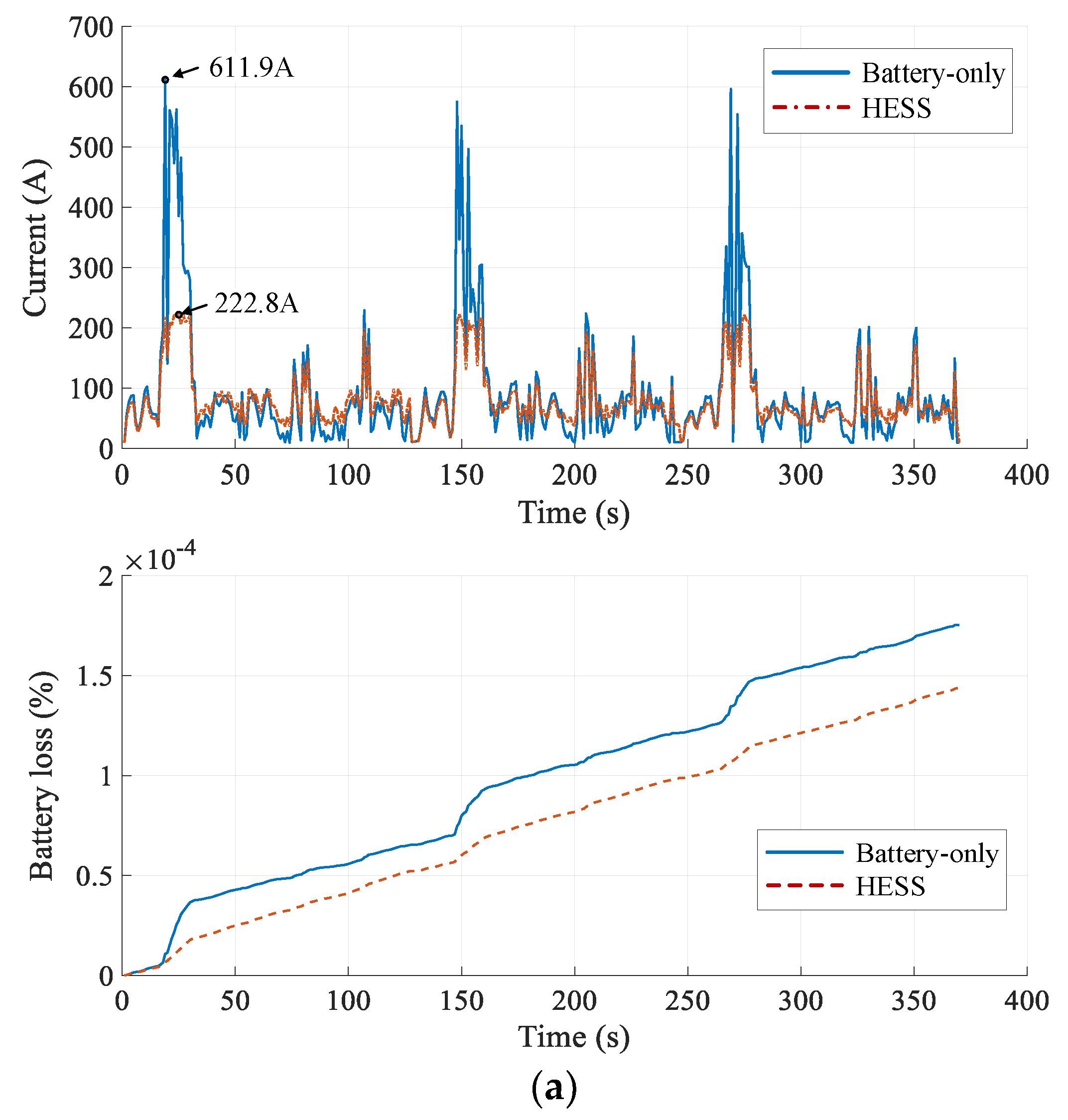
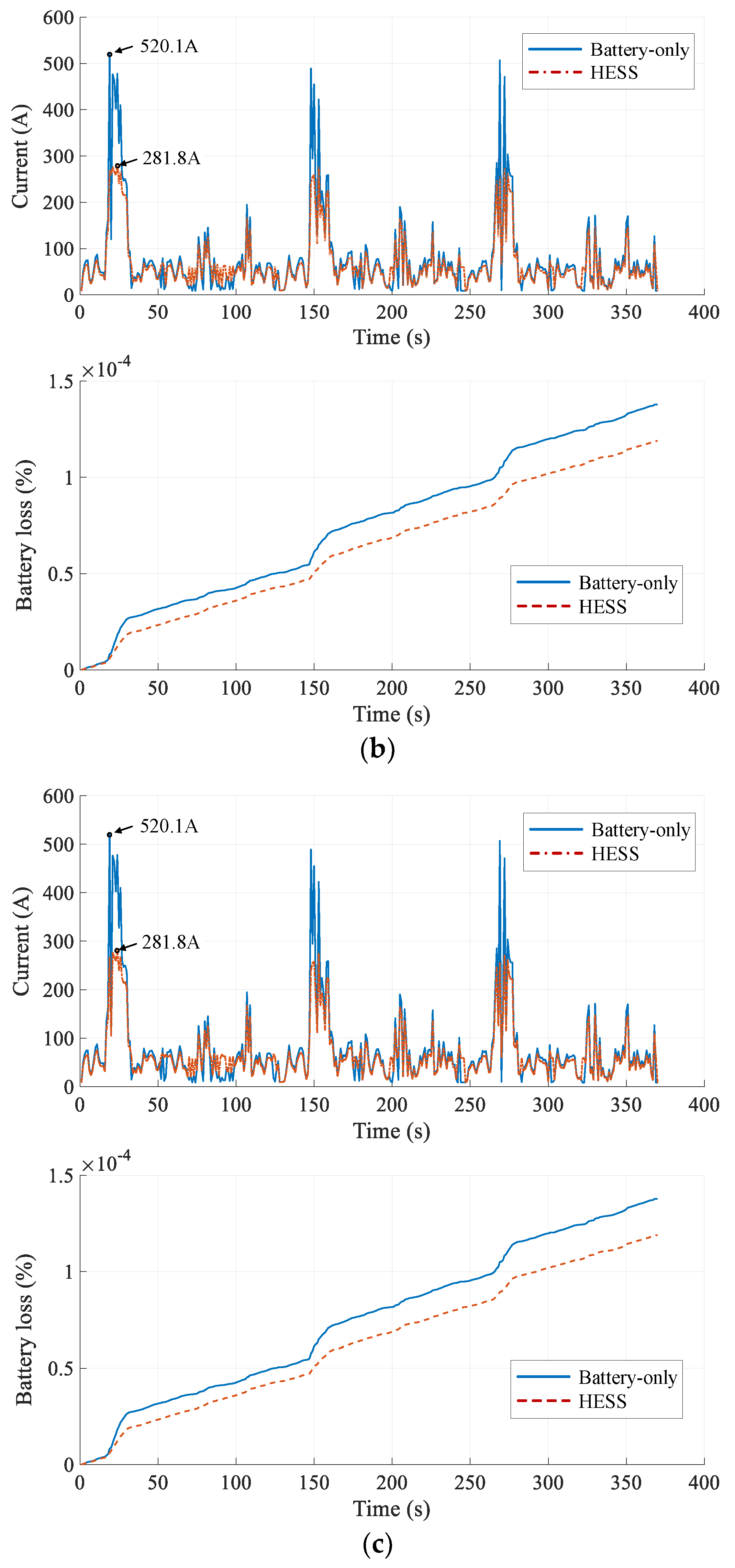
5.3. HESS vs. Battery-Only Options

To quantitatively compare the performances of both HESS optimal obtained by MSSR and battery-only options,

Table 8. The performances for both HESS and battery-only options.

Constraint	Option	LCC (€/day)	$\mathit{C}\mathit{o}\mathit{s}{\mathit{t}}_{\mathbf{c}\mathbf{a}\mathbf{p}}$ (€/day)	$\mathit{C}\mathit{o}\mathit{s}{\mathit{t}}_{\mathbf{o}\mathbf{p}\mathbf{e}}$ (€/day)	$\mathit{C}\mathit{o}\mathit{s}{\mathit{t}}_{\mathbf{r}\mathbf{e}\mathbf{p}}$ (€/day)	${\mathit{E}}_{\mathit{C}}$ (104 KJ)	${\mathit{Q}}_{\mathbf{l}\mathbf{o}\mathbf{s}\mathbf{s}}$ (10−4 %)	${\mathit{W}}_{\mathit{h}\mathit{r}\mathit{s}}$ (h)
$W_{\mathrm{hrs}}\ge 4$	HESS	194.07	50.47	32.52	111.07	1.6714	1.4371	4.07
	Battery-only	227.66	43.24	36.69	147.73	1.8855	1.7538	3.61
$W_{\mathrm{hrs}}\ge 5$	HESS	214.79	70.31	32.20	112.28	1.6547	1.1889	5.16
	Battery-only	269.97	65.28	36.68	168.01	1.8850	1.3784	4.53
$W_{\mathrm{hrs}}\ge 6$	HESS	214.89	70.44	32.17	112.28	1.6530	1.1874	6.08
	Battery-only	269.97	65.28	36.68	168.01	1.8850	1.3784	5.33

comprehensively shows the performances in three situations.

In addition, the battery current and capacity loss of the corresponding solutions are illustrated in Figure 14 to demonstrate the operation of the battery and its changes in capacity loss. It can be observed from the perspective of the LCC that the value of the optimal HESS solution is reduced by 14.76%, 20.44%, and 20.41%, respectively, compared to the battery-only counterparts. Although the Cost_cap will be lower in battery-only options (without UC), the battery peak current is increased by 63.59%, 45.82%, and 45.82%, respectively (see battery current in Figure 14), which will definitely enhance the Q_loss (18.06%, 13.75%, and 13.86%), presenting completely in the capacity loss in Figure 14, and thus raising the Cost_rep (24.82%, 33.17%, and 33.17%). In terms of the efficiency, solutions of HESS can also achieve better results since their flexible operation and capability to diminish the E_C (11.36%, 12.22%, and 12.31%) by effectively regulating the UC power. Less E_C leads to lower Cost_ope (11.37%, 12.21%, and 12.30%) for the reason that the cost is calculated directly by the energy consumption as exemplified in Equation (28), and as a result, the W_hrs of the HESS solutions are improved by 11.31%, 12.21%, and 12.34% compared to battery-only options.

Accordingly, HESS solutions exhibit better performances both in cost and efficiency when compared to battery-only options. After wholly considering the results in the three situations, it can be found that in HESS solutions the average reduction of the LCC is 18.54% and the average decrease of the E_c is 11.97%, which shows that HESS is a more economical and efficient option.

5.4. Comparison with Previous Work

The optimal solution selected from [8] is $N_{\mathrm{BT}}=200$, $M_{\mathrm{BT}}=6$, $N_{\mathrm{UC}}=15$, and $M_{\mathrm{UC}}=1$. The $DO{D}_{\mathrm{BT}}$ and the DC/DC converter efficiency were assumed as 100% and 95% at that time. Now, we still set the $DO{D}_{\mathrm{BT}}$ as 100%, use the DC/DC converter 3D efficiency map, and try to set other conditions as same as the ones in this paper. Due to the solution in [8] was designed to meet six hours of working time, therefore, the HESS solution for $W_{\mathrm{hrs}}\ge 6$ will be employed to make a comparison.

It can be clearly seen from

Table 9. The comparison results.

Solution	LCC (€/day)	Capital Cost (€/day)	Replacement Cost (€/day)	DODBT (%)	Whrs (h)
[8]	232.28	50.85	148.98	100	5.27
$W_{\mathrm{hrs}}\ge 6$	214.89	70.44	112.28	76.23	6.08

that compared to the solution in [8], solution $W_{\mathrm{hrs}}\ge 6$ obtained from MSSR has more advantages, including fewer LCC and replacement cost as well as longer working hours. The difference in DOD_BT can have a great impact on the results listed in the Table 9. In terms of the HESS optimization variables, solution $W_{\mathrm{hrs}}\ge 6$ has more batteries and UCs with narrower battery operating range, which can not only ensure the working hours but reduce the burden on batteries. On the other hand, although the capital cost of solution $W_{\mathrm{hrs}}\ge 6$ is higher, its replacement cost is fewer because of the longer battery life. Consequently, the comparison results indicate that the better solution can be attained by adding the DOD_BT as the new optimization variables and using the advanced MSSR based global optimization search method based on the HESS performance and power-loss model.

6. Conclusions

HESS presents as an ideal solution for the heavy-duty EVs with dynamic on-off loads to extend the life of the batteries and to reduce the LCC of the EVs. The design optimization of the HESS involves architecture selection, component size optimization, and EMS optimization, forming a very complex and challenging problem.

In this work, a nested, dual-level optimization problem has been formulated for the optimal design of HESS to minimize the LCC of electrified construction and mining vehicles with dynamic on-off loads. In the design optimization of the HESS, the DP-based optimal EMS aiming to achieve the minimum energy consumption in the HESS operation control optimization has been generated through the inner loop, lower level optimization; and the HESS component size optimization to achieve the minimum LCC using the performance and power-loss model of the HESS has been accomplished through the outer loop, higher level optimization. The formulated optimization problem has been solved using an advanced MSSR based global optimization search algorithm. Application of the method to the design optimization of the HESS of an LHD is used to demonstrate the capability and advantages of the new optimization problem formulation and solution method. The performance and costs of electrified LHD with optimized HESS and with pure battery ESS are compared quantitatively, showing the advantages of the HESS for the heavy-duty construction and mining vehicles.

References

1. Burke, A. Batteries and Ultracapacitors for Electric, Hybrid, and Fuel Cell Vehicles. Proc. IEEE 2007, 95, 806–820. [Google Scholar] [CrossRef]
2. Salisa, A.; Zhang, N.; Zhu, J. A comparative analysis of fuel economy and emissions between a conventional HEV and the UTS PHEV. IEEE Trans. Veh. Technol. 2011, 60, 44–54. [Google Scholar] [CrossRef]
3. Bilgin, B.; Magne, P.; Malysz, P.; Yang, Y.; Pantelic, V.; Preindl, M.; Korobkine, A.; Jiang, W.; Lawford, M.; Emadi, A. Making the case for electrified transportation. IEEE Trans. Transp. Electrif. 2015, 1, 4–17. [Google Scholar] [CrossRef]
4. Evans, A.; Strezov, V.; Evans, T. Assessment of utility energy storage options for increased renewable energy penetration. Renew. Sustain. Energy Rev. 2012, 16, 4141–4147. [Google Scholar] [CrossRef]
5. Zhao, H.; Wu, Q.; Hu, S.; Xu, H.; Rasmussen, C. Review of energy storage system for wind power integration support. Appl. Energy 2015, 137, 545–553. [Google Scholar] [CrossRef] [Green Version]
6. Lukic, S.; Jian, C.; Bansal, R.; Rodriguez, F.; Emadi, A. Energy Storage Systems for Automotive Applications. IEEE Trans. Ind. Electron. 2008, 55, 2258–2267. [Google Scholar] [CrossRef]
7. Hu, X.; Johannesson, L.; Murgovski, N.; Egardt, B. Longevity-conscious dimensioning and power management of the hybrid energy storage system in a fuel cell hybrid electric bus. Appl. Energy 2015, 137, 913–924. [Google Scholar] [CrossRef]
8. Liu, J.; Jin, T.; Liu, L.; Chen, Y.; Yuan, K. Multi-Objective Optimization of a Hybrid ESS Based on Optimal Energy Management Strategy for LHDs. Sustainability 2017, 9, 1874. [Google Scholar] [CrossRef]
9. Cao, J.; Emadi, A. A new battery/ultracapacitor hybrid energy storage system for electric, hybrid, and plug-in hybrid electric vehicles. IEEE Trans. Power Electron. 2012, 27, 122–132. [Google Scholar] [CrossRef]
10. Trovão, J.; Pereirinha, P.; Jorge, H.; Antunes, C. A multi-level energy management system for multi-source electric vehicles-An integrated rule-based meta-heuristic approach. Appl. Energy 2013, 105, 304–318. [Google Scholar] [CrossRef]
11. Masih-Tehrani, M.; Ha’iri-Yazdi, M.; Esfahanian, V.; Safaei, A. Optimum sizing and optimum energy management of a hybrid energy storage system for lithium battery life improvement. J. Power Sources 2013, 244, 2–10. [Google Scholar] [CrossRef]
12. Song, Z.; Li, J.; Han, X.; Xu, L.; Lu, L.; Ouyang, M.; Hofmann, H. Multi-objective optimization of a semi-active battery/supercapacitor energy storage system for electric vehicles. Appl. Energy 2014, 135, 212–224. [Google Scholar] [CrossRef]
13. Zhang, L.; Hu, X.; Wang, Z.; Sun, F.; Deng, J.; Dorrell, D. Multi-Objective Optimal Sizing of Hybrid Energy Storage System for Electric Vehicles. IEEE Trans. Veh. Technol. 2018, 67, 1027–1035. [Google Scholar] [CrossRef]
14. Hu, X.; Moura, S.; Murgovski, N.; Egardt, B.; Cao, D. Integrated Optimization of Battery Sizing, Charging, and Power Management in Plug-In Hybrid Electric Vehicles. IEEE Trans. Control Syst. Technol. 2016, 24, 1036–1043. [Google Scholar] [CrossRef] [Green Version]
15. Li, T.; Liu, H.; Zhao, D.; Wang, L. Design and analysis of a fuel cell supercapacitor hybrid construction vehicle. Int. J. Hydrogen Energy 2016, 41, 12307–12319. [Google Scholar] [CrossRef]
16. Cai, Q.; Brett, D.; Browning, D.; Brandon, N. A sizing-design methodology for hybrid fuel cell power systems and its application to an unmanned underwater vehicle. J. Power Sources 2010, 195, 6559–6569. [Google Scholar] [CrossRef]
17. Wu, X.; Cao, B.; Li, X.; Xu, J.; Ren, X. Component sizing optimization of plug-in hybrid electric vehicles. Appl. Energy 2011, 88, 799–804. [Google Scholar] [CrossRef]
18. Tani, A.; Camara, M.; Dakyo, B. Energy management based on frequency approach for hybrid electric vehicle applications: Fuel-cell/lithium-battery and ultracapacitors. IEEE Trans. Veh. Technol. 2012, 61, 3375–3386. [Google Scholar] [CrossRef]
19. Shen, J.; Dusmez, S.; Khaligh, A. Optimization of sizing and battery cycle life in battery/ultracapacitor hybrid energy storage systems for electric vehicle applications. IEEE Trans. Ind. Inform. 2014, 10, 2112–2121. [Google Scholar] [CrossRef]
20. Kim, M.; Peng, H. Power management and design optimization of fuel cell/battery hybrid vehicles. J. Power Sources 2007, 165, 819–832. [Google Scholar] [CrossRef] [Green Version]
21. Xu, L.; Mueller, C.; Li, J.; Ouyang, M.; Hu, Z. Multi-objective component sizing based on optimal energy management strategy of fuel cell electric vehicles. Appl. Energy 2015, 157, 664–674. [Google Scholar] [CrossRef]
22. Herrera, V.; Milo, A.; Gaztañaga, H.; Otadui, I.; Villarreal, I.; Camblong, H. Adaptive energy management strategy and optimal sizing applied on a battery-supercapacitor based tramway. Appl. Energy 2016, 169, 831–845. [Google Scholar] [CrossRef]
23. Hung, Y.; Wu, C. An integrated optimization approach for a hybrid energy system in electric vehicles. Appl. Energy 2012, 98, 479–490. [Google Scholar] [CrossRef]
24. Hung, Y.; Wu, C. A combined optimal sizing and energy management approach for hybrid in-wheel motors of EVs. Appl. Energy 2015, 139, 260–271. [Google Scholar] [CrossRef]
25. Murgovski, N.; Johannesson, L.; Sjöberg, J.; Egardt, B. Component sizing of a plug-in hybrid electric powertrain via convex optimization. Mechatronics 2012, 22, 106–120. [Google Scholar] [CrossRef] [Green Version]
26. Murgovski, N.; Johannesson, L.; Sjöberg, J. Engine On/Off Control for Dimensioning Hybrid Electric Powertrains via Convex Optimization. IEEE Trans. Veh. Technol. 2013, 62, 2949–2962. [Google Scholar] [CrossRef] [Green Version]
27. Murgovski, N.; Johannesson, L.; Egardt, B. Optimal Battery Dimensioning and Control of a CVT PHEV Powertrain. IEEE Trans. Veh. Technol. 2014, 63, 2151–2161. [Google Scholar] [CrossRef]
28. Hu, X.; Jiang, J.; Egardt, B.; Cao, D. Advanced power-source integration in hybrid electric vehicles: Multicriteria optimization approach. IEEE Trans. Ind. Electron. 2015, 62, 7847–7858. [Google Scholar] [CrossRef]
29. Holland, J. Adaptation in Natural and Artificial Systems; University of Michigan Press: Ann Arbor, MI, USA, 1975. [Google Scholar]
30. Ong, Y.; Nair, P.; Keane, A. Evolutionary optimization of computationally expensive problems via surrogate modeling. Am. Inst. Aeronaut. Astronaut. J. 2003, 41, 687–696. [Google Scholar] [CrossRef]
31. Zhou, Z.; Ong, Y.; Lim, M.; Lee, B. Memetic algorithm using multi-surrogates for computationally expensive optimization problems. Soft Comput. 2007, 11, 957–971. [Google Scholar] [CrossRef]
32. Dong, H.; Song, B.; Dong, Z.; Wang, P. Multi-start Space Reduction (MSSR) surrogate-based global optimization method. Struct. Multidiscip. Optim. 2016, 54, 907–926. [Google Scholar] [CrossRef]
33. Zheng, J.; Jow, T.; Ding, M. Hybrid power sources for pulsed current applications. IEEE Trans. Aerosp. Electron. Syst. 2001, 37, 288–292. [Google Scholar] [CrossRef]
34. Napoli, A.; Crescimbini, F.; Capponi, F.; Solero, L. Control strategy for multiple input DC-DC power converters devoted to hybrid vehicle propulsion systems. Proc. IEEE Int. Symp. Ind. Electron. 2002, 3, 1036–1041. [Google Scholar]
35. Ortúzar, M.; Moreno, J.; Dixon, J. Ultracapacitor-based auxiliary energy system for an electric vehicle: Implementation and evaluation. IEEE Trans. Ind. Electron. 2007, 54, 2147–2156. [Google Scholar] [CrossRef]
36. Spotnitz, R. Simulation of capacity fade in lithium-ion batteries. J. Power Sources 2003, 113, 72–80. [Google Scholar] [CrossRef]
37. Ramadass, P.; Haran, B.; Gomadam, P.; White, R.; Popov, B. Development of first principles capacity fade model for Li-ion cells. J. Electrochem. Soc. 2004, 151, A196–A203. [Google Scholar] [CrossRef]
38. Wang, J.; Liu, P.; Garner, J.; Sherman, E.; Soukiazian, S.; Verbrugge, M.; Tataria, H.; Musser, J.; Finamore, P. Cycle-life model for graphite-LiFePO4 cells. J. Power Sources 2011, 196, 3942–3948. [Google Scholar] [CrossRef]
39. Bloom, I.; Cole, B.; Sohn, J.; Jones, S.; Polzin, E.; Battaglia, V.; Henriksen, G.; Motloch, C.; Richardson, R.; Unkelhaeuser, T.; et al. An accelerated calendar and cycle life study of Li-ion cells. J. Power Sources 2001, 101, 238–247. [Google Scholar] [CrossRef]
40. Plett, G. Extended Kalman filtering for battery management systems of LiPB-based HEV battery packs Part 2. Modeling and identification. J. Power Sources 2004, 134, 262–276. [Google Scholar] [CrossRef]
41. Kong, X.; Choi, L.; Khambadkone, A. Analysis and control of isolated current-fed full bridge converter in fuel cell system. In Proceedings of the 30th Annual Conference of IEEE Industrial Electronics Society (IECON 2004), Busan, Korea, 2–6 November 2004. [Google Scholar]
42. Ansarey, M.; Panahi, M.; Ziarati, H.; Mahjoob, M. Optimal energy management in a dual-storage fuel-cell hybrid vehicle using multi-dimensional dynamic programming. J. Power Sources 2014, 250, 359–371. [Google Scholar] [CrossRef]
43. Santucci, A.; Sorniotti, A.; Lekakou, C. Power split strategies for hybrid energy storage systems for vehicular applications. J. Power Sources 2014, 258, 395–407. [Google Scholar] [CrossRef]
44. Song, Z.; Hofmann, H.; Li, J.; Han, X.; Ouyang, M. Optimization for a hybrid energy storage system in electric vehicles using dynamic programing approach. Appl. Energy 2015, 139, 151–162. [Google Scholar] [CrossRef]
45. Zakeri, B.; Syri, S. Electrical energy storage systems: A comparative life cycle cost analysis. Renew. Sustain. Energy Rev. 2015, 42, 569–596. [Google Scholar] [CrossRef]
46. Man, K.; Tang, K.; Kwong, S. Genetic algorithms: Concepts and applications [in engineering design]. IEEE Trans. Ind. Electron. 1996, 43, 519–534. [Google Scholar] [CrossRef]
47. Montazeri-Gh, M.; Poursamad, A.; Ghalichi, B. Application of genetic algorithm for optimization of control strategy in parallel hybrid electric vehicles. J. Frankl. Inst. 2006, 343, 420–435. [Google Scholar] [CrossRef]
48. Jacobs, W.; Hodkiewicz, M.; Bräunl, T. A Cost-Benefit Analysis of Electric Loaders to Reduce Diesel Emissions in Underground Hard Rock Mines. IEEE Trans. Ind. Electron. 2015, 51, 2565–2573. [Google Scholar] [CrossRef]
Figure 1. Semi-active HESS topology.
Energies 11 02699 g001
Figure 2. Relationship between the battery capacity vs. cycles: (a) at different DOD (C/2); (b) at different C-rate (80% DOD).
Energies 11 02699 g002
Figure 3. Equivalent circuit models: (a) battery cell; and (b) UC module.
Energies 11 02699 g003
Figure 4. Voltage doubler boost converter.
Energies 11 02699 g004
Figure 5. Switch voltage and current.
Energies 11 02699 g005
Figure 6. Structure of the nested optimization framework.
Energies 11 02699 g006
Figure 7. Driving cycle of LHDs.
Energies 11 02699 g007
Figure 8. Power demand of an LHD.
Energies 11 02699 g008
Figure 9. DC/DC converter efficiency map.
Energies 11 02699 g009
Figure 10. Iterative results of GA.
Energies 11 02699 g010
Figure 11. Iterative results of MSSR.
Energies 11 02699 g011
Figure 12. Iterative results of MSSR: (a) 5 h; (b) 6 h.
Energies 11 02699 g012
Figure 13. UC voltage and battery power in three situations: (a) 4 h; (b) 5 h; and (c) 6 h.
Energies 11 02699 g013aEnergies 11 02699 g013b
Figure 14. Battery current and capacity loss in three situations: (a) 4 h; (b) 5 h; and (c) 6 h.
Energies 11 02699 g014aEnergies 11 02699 g014b