Abstract
To improve the reliability and reduce power loss of distribution network, the dynamic reconfiguration is widely used. It is employed to find an optimal topology for each time interval while satisfying all the physical constraints. Dynamic reconfiguration is a non-deterministic polynomial problem, which is difficult to find the optimal control strategy in a short time. The conventional methods solved complex model of dynamic reconfiguration in different ways, but only local optimal solutions can be found. In this paper, a data-driven optimization control for dynamic reconfiguration of distribution network is proposed. Through two stages that include rough matching and fine matching, the historical cases which are similar to current case are chosen as candidate cases. The optimal control strategy suitable for the current case is selected according to dynamic time warping (DTW) distances which evaluate the similarity between the candidate cases and the current case. The advantage of the proposed approach is that it does not need to solve complex model of dynamic reconfiguration, and only uses historical data to obtain the optimal control strategy for the current case. The cases study shows that the optimization results and the computation time of the proposed approach are superior to conventional methods.
1. Introduction
The reconfiguration of distribution network is an important mean to improve the reliability and economy of the distribution network by opening the normally closed sectionalizing switches and subsequently closing the normally open switches. The reconfiguration of distribution network can be divided into static reconfiguration and dynamic reconfiguration according to the different optimization time scales.
The static reconfiguration of distribution network is a multi-objective nonlinear hybrid optimization problem that focuses on one determined time point. The optimization process requires a lot of computing time because of its nonlinear characteristics. In addition, the static reconfiguration neglects the conditions such as load changes and switch operation constraints, which are difficult to apply directly in practical projects. So far, many scholars have proposed various algorithms to solve static reconfiguration. The traditional methods mainly include newton method, quadratic programming, artificial neural network, interior point method, heuristic algorithm and so on. Gomes Fonseca proposed an analysis tool for static reconfiguration of distribution network based on the fast decoupled newton-raphson power flow method [1]. This method uses the information of the state of the network and does not require previous topology processing. H.P. Schmidt developed a new quadratic formulation for reconfiguration of distribution systems [2]. It guarantees the global minimum is unique and hence allows an efficient application of the standard newton method. A mixed-integer quadratically constrained convex optimization program is implemented in distribution network by R. Fakhry, which overcomes the main shortcomings of artificial intelligence techniques [3]. K. Sathish Kumar presented a modified artificial neural network for identifying best switching option to reduce power loss [4]. JA Momoh proposed a fast integer interior point programming method which incorporated the interior point linear programming technique with branch and bound technique to optimize the reconfiguration problem [5]. Arash Asrari proposed a systematic approach to determine an optimal long-term reconfiguration schedule based on a novel adaptive fuzzy-based parallel genetic algorithm [6]. In order to combine problem of network reconfiguration and capacitor placement simultaneously in the presence of non-linear loads, Fahimeh Sayadi proposed a new particle swarm optimization algorithm [7]. Although many scholars did a lot of work on static reconfiguration of distribution network, there are still many problems with these traditional methods. For example, the quadratic programming method has the problem of large computation and poor convergence. Newton method has good convergence performance, but cannot deal with a large number of inequality constraints. The artificial neural network method has the disadvantage of relying too much on the sample. The interior point method is difficult to handle the infeasible solutions generated in the optimization process. Heuristic algorithm has the long computing time and easy to get into local optimal solution. In general, when traditional methods are applied to solve complex dynamic reconfiguration models, they will consume a lot of computation time and not easy to get the global optimal solution.
On the contrary, the dynamic reconfiguration of distribution network can change the state of switches with load variation and switch operation constraints. In this case, it can ensure that the distribution network operates in a safe, high-quality and economic friendly environment, which is more in accordance with the requirements of the actual operation scheduling compared with static reconfiguration. At present, most of the articles divided dynamic reconfiguration of distribution network into two steps. The first step is to divide one day into several time intervals and the second step is to deal with static reconfiguration in each time interval. Xiaoli Meng proposed a dynamic reconfiguration method of distribution network with large-scale distributed generation integration. The whole time period is divided into several time intervals by fuzzy clustering analysis method [8]. Lizhou Xu used power losses and static voltage stability index to get the time intervals of dynamic reconfiguration [9]. Huping Yang proposed a gradual approaching method to deal well with dynamic reconfiguration. The optimal time for reconfiguration is determined by time enumeration method [10]. Zhenkun Li presented a multi-agent system that divided one day into o several time intervals and each was managed by a work agent [11]. In general, the existing dynamic reconfiguration strategies have the following shortcomings: (1) the number of time intervals needs to be set artificially, which is very subjective. Some scholars used enumeration method to find the optimal number of intervals, but it leads to a large amount of computation time. It is hard to find the optimal number of time intervals within a short time. (2) some traditional methods of solving static reconfiguration can find the optimal solution, but they also need very long computation time.
The distribution network generates massive amounts of data every day. It can be collected by sensors and stored in the database. When the amount of data accumulated in the database is large enough, the load series in the future may be very similar to the historical load series. In this case, the large amounts of historical data make it possible to establish data-driven models for optimization of distribution network. Ziqiang Zhou proposed a data-driven approach to forecast photovoltaic power, which was instructive for distribution network planning and energy policy making [12]. A data-driven approach to fault detection in smart distribution grids was proposed by Younes Seyedi [13]. Simulation results confirmed that the proposed networked protection approach can effectively detect faults within pre-defined fault tolerance time. To determine the maximum penetration level of distributed generation for active distribution networks, Xin Chen proposed a data-driven method based on distributional robust optimization [14]. However, the research on dynamic reconfiguration of distribution network based on data-driven models is relatively limited.
In this paper, a data-driven optimization control for dynamic reconfiguration of distribution network is proposed. Through two stages of rough matching and fine matching, the historical cases similar to current case are chosen as candidate cases. The optimal control strategy suitable for the current case is selected according to dynamic time warping distances which evaluate the similarity between the candidate cases and the current case. The key contributions of this paper are as follows:
- (1)
- The proposed approach does not need to solve complex model of dynamic reconfiguration, and only uses historical data to obtain the optimal control strategy for the current case. In addition, the proposed approach is faster than most of traditional methods in term of computation time.
- (2)
- Some traditional methods such as enumeration can find the optimal strategy for dynamic reconfiguration, but it will consume a lot of computation time, which is not suitable for real-time control of distribution network. In addition, these optimal strategies that take a lot of time to find will not be reused in the future, wasting a lot of potentially valuable data. The proposed approach can make full use of the value of historical data, recycling the optimal strategies of historical cases.
- (3)
- Traditional algorithms such as heuristic algorithms find control strategies that tend to be approximate optimal solutions, but they can’t figure out the probability that the selected control strategy is the optimal strategy for the current case. In contrast, the probability can be obtained by proposed approach according to dynamic time warping distance between historical case and current case.
The rest of this paper is organized as follows. Section 2 presents the mathematical model of dynamic reconfiguration. Section 3 proposes how to quickly select a historical case similar to current case from the database. Section 4 discusses the simulations and results. The conclusion is described in Section 5.
2. The Mathematical Model of Dynamic Reconfiguration
2.1. Objective Function
The objective function of dynamic reconfiguration is to minimize the total costs which include the power loss costs and switching costs. The total costs can be expressed as follows:
where: F is the comprehensive costs of total time intervals; T is the number of time intervals; is the power prices of time interval t; is the power loss of time interval t; t is the span of time interval; is the amount of feasible switches motion; is the unit price of one switch motion; is the state of switch i in the time intervals which 1 means switch closed and 0 represents switch open.
2.2. Equality Constraints and Inequality Constraints
The objective function needs to satisfy many constraints, such as security, technical and topological constraints. The equality constraints include two nonlinear recursive power flow equations, and it can be expressed as follows:
where: is the active power of node i; is the reactive power of node i; is voltage of node i; N is the number of nodes; is conductance of branch between node i and node j; is the susceptance of branch between node i and node j; is the angle difference between node i and node j.
The voltages limit and electric current limit can be expressed as follows:
where: N is the number of nodes; M is the number of branch.
The constraints of number of switch motion times can be expressed as follows:
where: is the largest motion time of single switch and is the largest motion time of all switches.
In addition, the objective function needs to satisfy constraint of network topology. The distribution network is connected radially without the presence of islanding after dynamic reconfiguration.
3. Dynamic Reconfiguration Based on Data-Driven Model
3.1. The Framework of the Proposed Approach
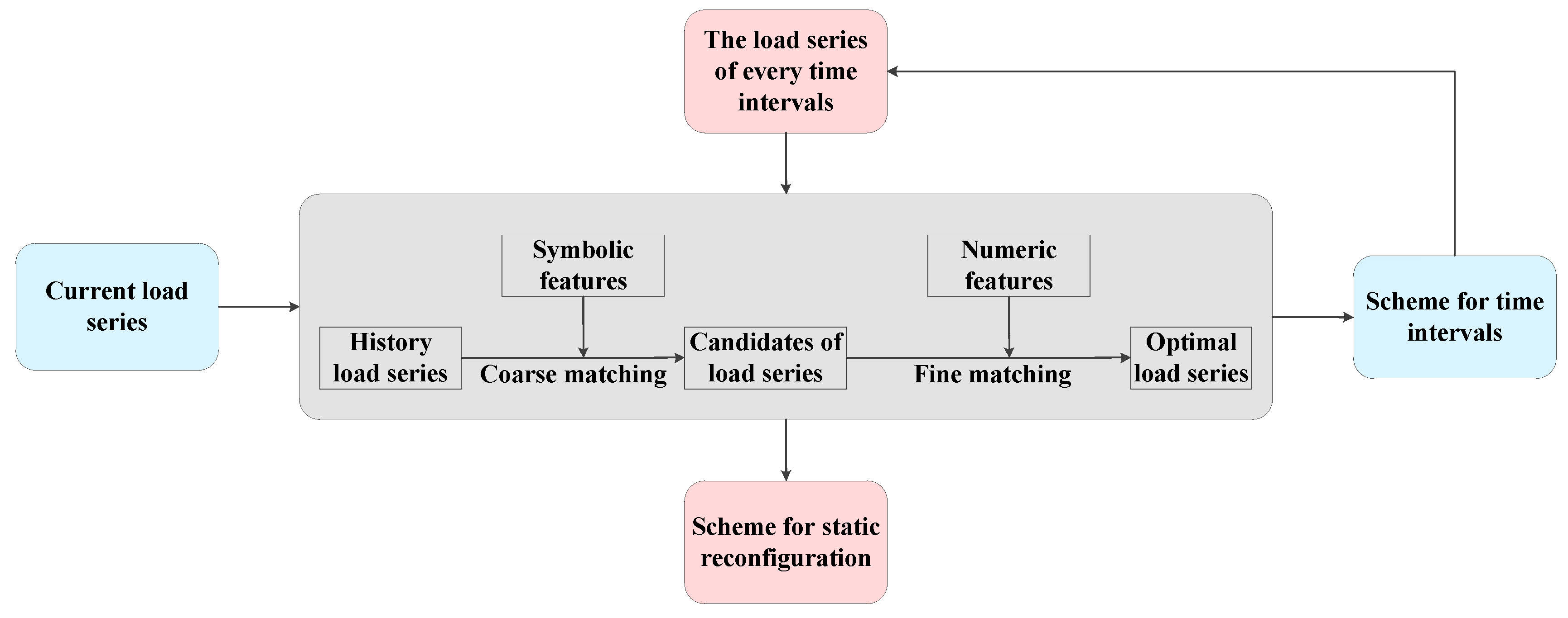
The dynamic reconfiguration of distribution network can be divided into two steps which include dividing time intervals and static reconfiguration. The first step is to divide one day into several time intervals and the second step is to deal with static reconfiguration in each time interval. The framework of data-driven model is shown in Figure 1.
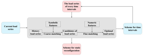
Figure 1.
The framework of proposed approach.
Scheme for dividing time intervals: First of all, several candidates of load curves are screened out in coarse matching stage according to the symbolic features of the load curves of the distribution network. Next, the numeric features of the candidates of load curves will be extracted by piecewise aggregate approximation. The dynamic time warping is calculated to evaluate the similarity between the current load curve and the candidates of load curves, and the optimal scheme for time intervals is selected according to dynamic time warping distance.
Scheme for static reconfiguration: For one thing, calculating the mean load for each node in every time interval and several candidates of load series are screened out in coarse matching stage according to the symbolic features of the load series. For another thing, taking the load of each node as the original feature, the principal component analysis is used to reduce the dimension of the numeric features whose weights are determined by entropy weight method. The dynamic time warping is calculated to evaluate the similarity between the current load series and the candidates of load series, and the optimal scheme for static reconfiguration is selected according to dynamic time warping distance. Different from the dividing time intervals, if the selected strategy is applied to distribution network directly, it may cause some inequality constraints to be unsatisfied. Therefore, we need to apply the selected strategy to the distribution network and then calculate the power flow. If all constraints are met, the selected strategy can be used. Otherwise, reselect the strategy in the remaining cases and then check if the constraints are met.
Obviously, implementing the proposed approach requires sufficient historical cases in the database. If the case in the database is insufficient, we need to simulate the load profiles based on historical data and then expand the case. For an actual distribution network, we can try to test the proposed algorithm using historical data for one year. If the testing result is not good, we can try to increase the historical data or simulate the load to expand the database.
When the network expansion faces faults, we need to do additional processing on the database. For network expansion, the network adds some power lines and loads. We need to simulate the load profiles each node and then find the optimal control strategy under various scenes. For lines faults, the network deletes some power lines and loads, we only need to re-solve the optimal control strategy for the historical data. Finally, the simulation case and the corresponding strategy are saved in the database.
3.2. Features Extraction
1. Features for time intervals
The load series can be obtained by sampling the daily load curve of the distribution network. If the sampling frequency is high, we can get a high-dimensional load series, which will consume a lot of time if we directly calculate the similarity between the load series. Therefore, it is necessary to extract the features of the original load series. The main information of the original load series can be reflected by a small number of features.
At present, many scholars have put forward plenty of methods to extract features, such as piecewise linear approximation, piecewise quadratic approximation and piecewise aggregate approximation [15]. Compared with other methods, the piecewise aggregate approximation has the advantages of fast calculation speed, and low dimension, which is widely used for time series analysis. So the piecewise aggregate approximation will be used to extract the features of load series. This method divides the load series of length n into k features of equal size [16]. Then it computes the mean value of the points inside each feature using the formula:
As we can see from the Figure 2, the initial load series of length 72 is reduced to 12 features which reflect the overall trend of the original load series. In fact, the more the number of features, the more detailed about the trend of the original load series can be described. But analysis and data mining of the load series will become very difficult because of the features with high dimension. Therefore, the number of features is also very important to the result, which can be obtained by empirical formula or experiment.
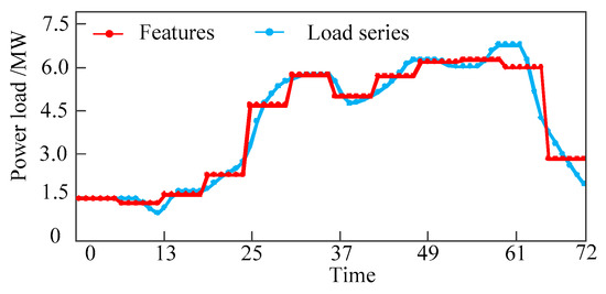
Figure 2.
The features are extracted by piecewise aggregate approximation.
2. Features for static reconfiguration
When the load of distribution network fluctuates greatly, the topology of the distribution network is changed by switching the state of switches, so as to affect the power flow of the network and achieve the purpose of optimizing operation. Figure 3 shows the power loss, voltages and the daily load curve of a distribution network.
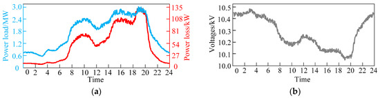
Figure 3.
The parameters of the distribution network: (a) The daily load curve and power loss of distribution network; (b) the voltages of distribution network.
As can be seen from Figure 3, the trends of power loss and load curve are roughly the same. When the load is heavy, the voltage of the node drops. On the contrary, if the load is light, the voltages will rise. In short, the power loss, voltages and power load have a strong correlation. When the distribution network load level is similar, the distribution network can use a similar topology to control the direction of power flow, so that the distribution network can operate in a safe and economic environment. Therefore, the power load of each node is selected as the original feature of static reconfiguration to evaluate the similarity between the current case and historical cases.
3.3. Dimensions and Weights of Features
According to the previous analysis, the power load of each node is selected as the original feature of static reconfiguration. As the number of nodes in the distribution network increases, the number of features also increases sharply, resulting in a large amount of computation time. It is necessary to reduce the dimension of features. In addition, each feature has different roles and influences, so it should be given a reasonable weight based on the function of each feature. Weight reflects the importance of each feature when calculating similarity, which is related to the contribution of each feature to global similarity. Therefore, it is important to determine the weight of each feature when calculating the similarity.
1. Principal component analysis
Principal component analysis is a statistical method that uses as few features as possible to reflect the original features on the basis of minimizing the loss of the original information. For example, the principal component analysis is applied to the covariance matrix of distributed wind power data in [17]. The principal component analysis was used to investigate dependency in transmission network flows in [18]. The main steps of principal component analysis are as follows:
(1) Normalization
In order to eliminate the impact of the units of the various features, the features should be normalized before using the principal component analysis. The features are normalized to get the matrix of by the method of min-max normalization [19]. Where: m is the number of historical cases; p is the number of features; is the feature after normalization.
(2) Calculating correlation matrix
The correlation matrix consists of elements that can be represented by . Each element is a correlation coefficient between two features, which can be expressed as follows:
where: is the mean of feature i; is the correlation coefficient between feature i and feature j.
(3) Calculating the new features
The eigenvalues of the correlation matrix are calculated and the eigenvalues are sorted in descending order. In addition, the eigenvectors corresponding to each eigenvalue are calculated. In order to ensure that the loss of the original information is as small as possible, the number of the principal components (the new features) should not be too small. The cumulative contribution ratio will be calculated to control the number of principal components. If the cumulative contribution ratio is greater than 85%, it can be considered that the new features can reflect the main information of the original features [17]. The cumulative contribution ratio can be expressed as follows:
where: is the eigenvalue; is the cumulative contribution ratio of the top m eigenvalues.
The ith new feature can be expressed as follows:
where: is the jth element of the ith eigenvectors.
2. Entropy weight method
The methods for determining weight can be divided into two types: objective methods and subjective methods. Among them, analytic hierarchy process is a typical subjective method, which depends on experience to determine weights. Because the physical meanings of the new features are not clear and the number of features is large, the subjective method is difficult to determine the weights. In this paper, the weight of each feature is determined by the entropy weight method which determines the weight according to the information contained in each feature. The calculation of entropy method is simple and fully utilizes the data to overcome the difficulty of determining the weights when the physical meaning of the features is not clear.
If the number of new features is n, the matrix of new features becomes . The information entropy of each feature can be expressed as follows:
where: is the information entropy of jth feature. The smaller the information entropy, the greater the role it plays in calculating the similarity. The weight of the jth feature can be expressed as follows:
3.4. Similarity Search
After extracting features, it is important to use features to search for historical cases that are most similar to current case. Sequential scanning is one of the most common and direct search methods. It calculates the similarity between the current case and all the historical cases one by one until finding the best historical cases. However, if the number of historical cases is enormous, the efficiency of the Sequential scanning is very low and the computation time will be very long.
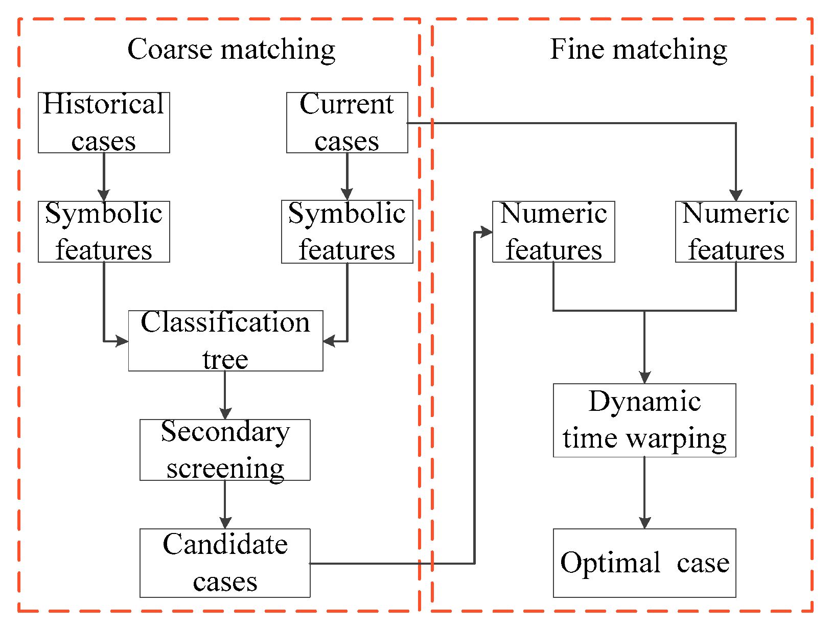
In order to improve the efficiency, as shown in Figure 4, this paper divides the search strategy into two steps which include coarse matching and fine matching.
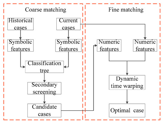
Figure 4.
Coarse matching and fine matching.
1. Coarse matching
According to the symbolic features of historical cases, several candidate cases similar to the current case are screened out by classification tree. However, the number of candidate cases is still very large. The candidate cases are screened twice by setting threshold.
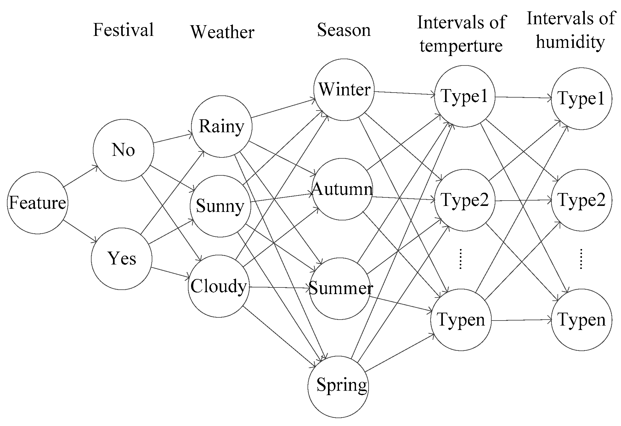
The power load of residents is affected by factors such as holidays, weather and other factors. The power load has some similarity in the same environment. For example, the residential load can be forecasted by historical days that the factors are similar, such as the lowest temperature, the highest temperature, the average temperature, humidity, and so on [20]. As shown in Figure 5, the historical cases can be described with seasons, holidays, weather and other symbolic features, and the historical cases can be primarily screened according to the symbolic features.
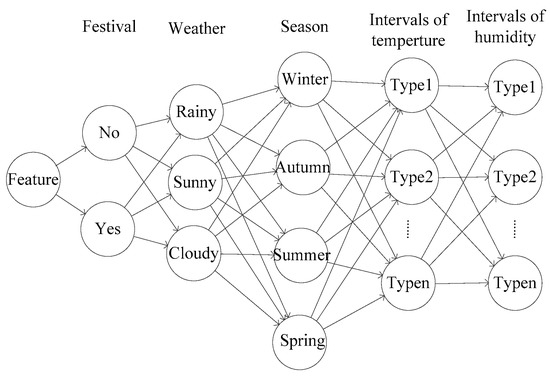
Figure 5.
Classification tree.
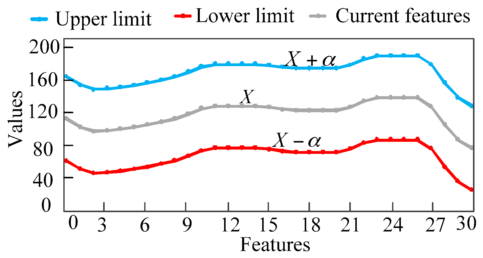
historical cases which are similar to the current case will be selected by the classification tree. In order to reduce the computational tasks, the historical cases are screened two times by setting a threshold. As shown in Figure 6, set the allowable deviation of the feature as , and exclude the candidate cases whose values of features fall outside the allowable range to further reduce the number of candidate cases. If the number of candidate cases is large, can be set smaller to exclude candidate cases that are not very similar to the current one. On the contrary, if the number of candidate cases is small, can be set to a larger size to avoid all candidate cases being excluded. If it is difficult to determine the value of in the first place, dichotomy can be used to quickly determine the size of .

Figure 6.
The second screening rules.
2. Fine matching
After screening candidate cases, it is also important to use numerical features to find the historical case that is most similar to the current case. So far, scholars have proposed many different methods to discover the similarities or hidden trends of time-series data. The most used distance measures are: Euclidean Distance (ED), Dynamic Time Warping (DTW), Singular Value Decomposition (SVD), and Point Distribution (PD). The ED and its variations are very sensitive to the small distortion of time and cannot adapt to the data conversion of the time axis [21]. SVD and PD are the methods for calculating similarity based on statistics. They do not consider the actual shape of load series. With different constraints applied to the search, DTW can tolerate different degrees of time distortion, or exclude unreasonable cases to reduce the search time [22].
The dynamic time warping is used to evaluate the similarity between the candidate cases and the current case, and the optimal control scheme suitable for the current case is selected according to dynamic time warping. Given two load series of X and Y which have length m and n respectively:
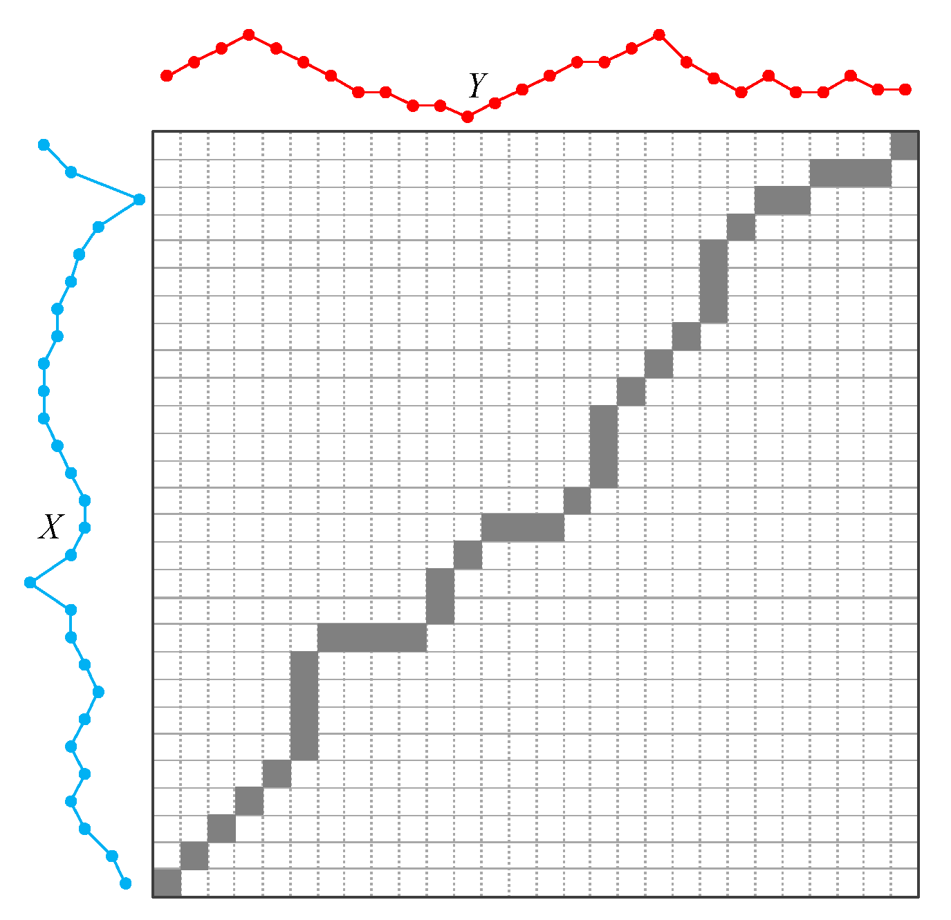
As shown in Figure 7, the DTW attempts to find a best warping paths with a minimum distance value. First, it needs to construct a matrix D with size . We can calculate the every element of the matrix as follows:
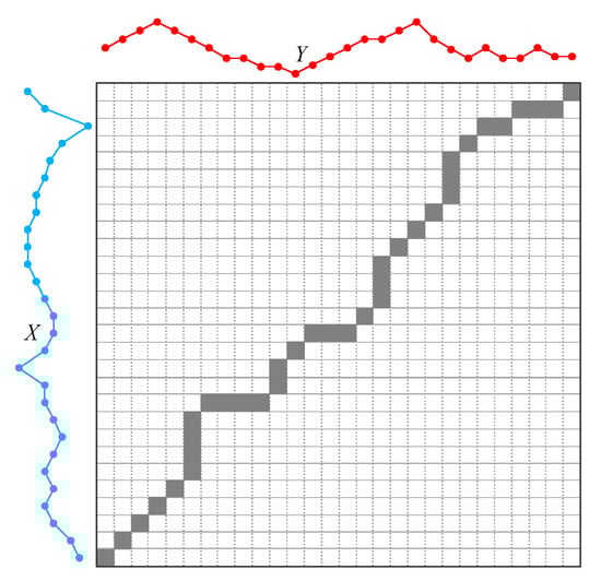
Figure 7.
The DTW distance.
The matrix D needs to be calculated as order of the above formula. It must calculate D(1,1) first, then D(i,1), D(1,j) and calculate D(i,j) at last. In this case, the distance between X and Y can be expressed as follows:
In addition, some constrains of DTW are proposed to accelerate computational time. For more detail about DTW and its constraints, readers can refer to [23].
3.5. Processing of Approaches
Summarizing the above analyses, the steps to implement the proposed algorithm are as follows:
Step 1: Import current power load and extract features.
Step 2: The principal component analysis is used to reduce the dimension of the feature, and then the weight of each feature is determined based on the entropy weight method.
Step 3: In the stage of coarse matching, several historical candidate cases are selected according to the symbol features.
Step 4: In the stage of fine matching, the dynamic time warping distance between candidate cases and the current case are calculated according to the numerical feature, and the candidate cases are sorted based on the dynamic time warping distance.
Step 5: The strategy of the candidate case with the smallest dynamic time warping distance is selected.
Step 6: The selected strategy is applied to the distribution network and the power flow is calculated. Determine if the distribution network meets all constraints.
Step 7: If all constraints are met, the chosen strategy is available. Otherwise, return to step 5.
3.6. Indicators for Evaluating Results
The results are evaluated by the indexes of accuracy rate, compression rate and satisfaction. The cases which are the most similar to the current case are selected from the database. The comprehensive costs of the schemes of dynamic reconfiguration are calculated respectively at current load level. Among them, comprehensive costs belong to the optimal solution at the current load level. The accuracy rate can be expressed as follows:
If is the optimal solution of comprehensive costs, is the worst solution of comprehensive costs. The satisfaction of current case can be expressed as follows:
It is assumed that principal component analysis transforms the dimension of feature from n to m. The compression rate can be calculated as follows:
4. Study Case
4.1. Setting Parameters
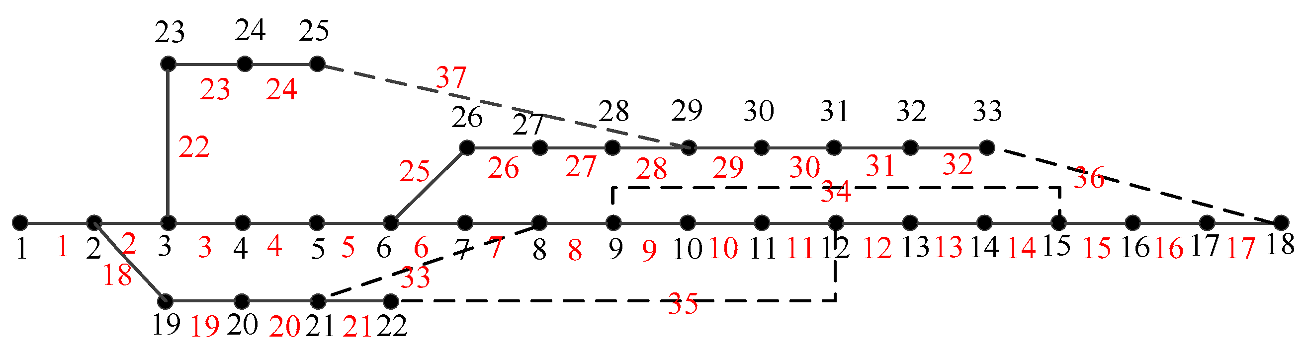
The proposed method will be tested on modified IEEE 33-bus system whose topology can be seen in Figure 8. For more detail about the parameters of branch, readers can refer to [24]. The hourly load factor is derived from Karnataka Power Transmission Corporation Limited, which contains actual historical data from 2010 to 2017. The largest motion time of single switch is 3 and the largest motion time of all switches is 15. The energy purchased price is 0.11$/kWh, and the switch motion cost is 1.11$/time. The dynamic reconfiguration strategy of historical cases belong to the global optimal solution which obtained by enumeration method. The algorithms were implemented by MATLAB R2014a, Windows7, Intel(R) Core(TM) i3-3110M CPU@2.40GHz,6.00 G RAM.
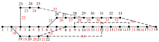
Figure 8.
The topology of modified IEEE 33-bus system.
4.2. The Results of the Time Intervals
1. Compared with traditional algorithms
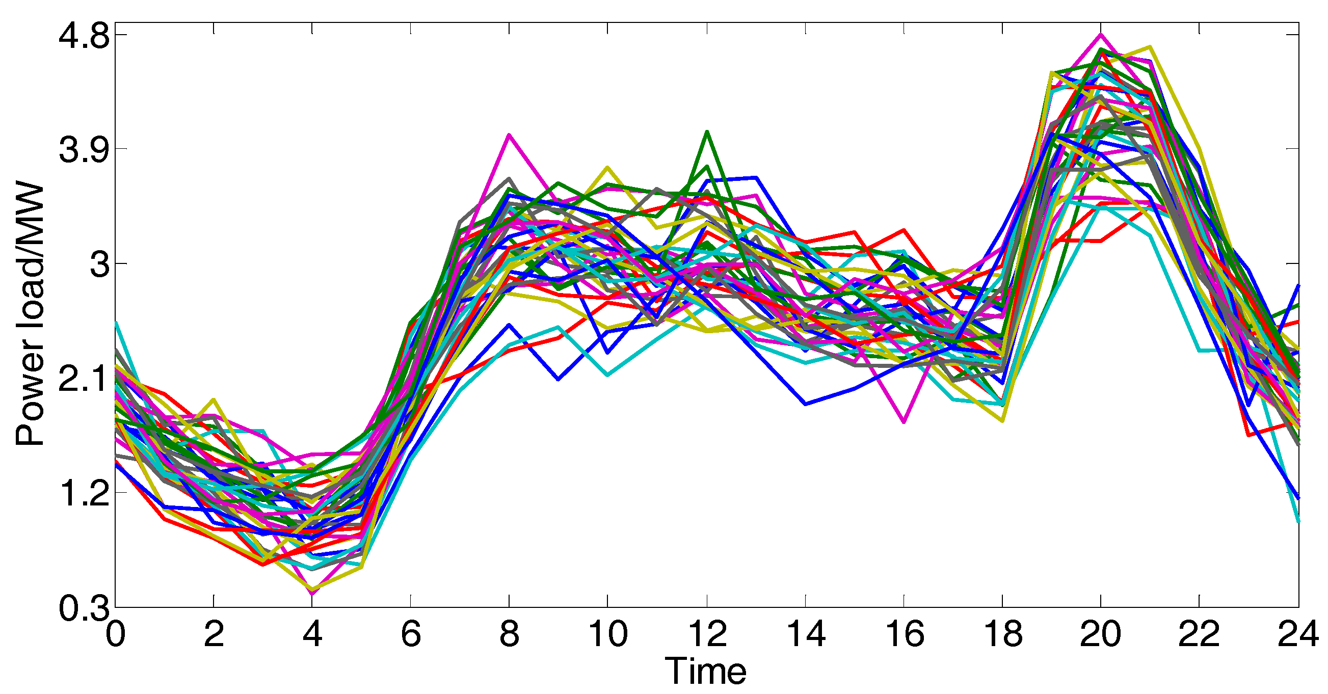
We choose one day in 2017 as the current case randomly and use the classification tree to select 240 candidate cases according to the symbolic features. Taking 1 h as the step size, 48 numeric features of each load series are extracted by piecewise aggregate approximation. As shown in Figure 9, the threshold is set to 0.1 by dichotomy, and 37 candidate cases are screened out.
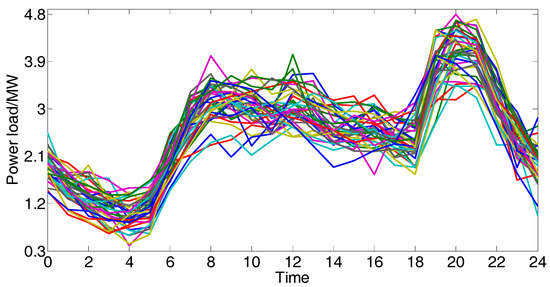
Figure 9.
The 37 candidate cases which are similar to the current case.
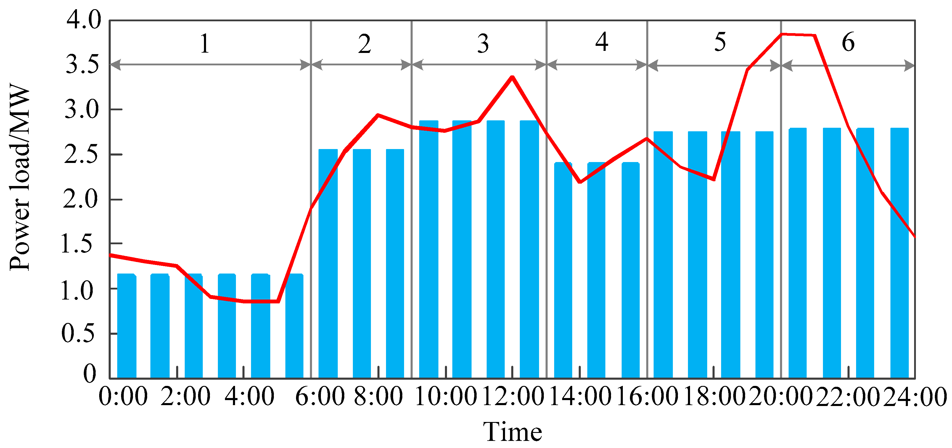
The schemes of the candidate cases are calculated based on a gradual approaching method which determined the time intervals by time enumeration method [10]. The dynamic time warping between the current case and the candidate cases are calculated and the scheme of the candidate case with the smallest dynamic time warping will be used to divide one day into several time intervals. As shown in Figure 10, the daily load curve is finally divided into six time intervals, and the results are basically in line with the trend of the curve.
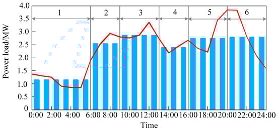
Figure 10.
The scheme that one day are divided into 6 time intervals.
In order to verify the reasonableness and correctness of the time intervals based on data-driven model, the following four schemes are used for simulation. Case A: Maintain the original topology without reconfiguration. Case B: The whole time period is divided into several time intervals by fuzzy clustering analysis method [8]. Case C: The whole time period is divided into several time intervals based on the indexes of power losses and static voltage stability [9]. Case D: one day is divided into several time intervals based on data-driven model. The four cases are optimized respectively and the results are shown in Table 1.

Table 1.
The comparison of optimized results from different cases.
As shown in Table 1, the power loss of case A which maintains the original topology without reconfiguration is 2716.3 kW, and its total cost is 301.3$. In case B, the power loss is reduced to 1954.6 kW through 12 switching operations. The total cost is reduced to 230.1$. The number of switching operations of case C is 10. Its power loss is 1983.9 kW and the total cost is 231.1$. In case D, the power loss is reduced to 1954.6 kW through 6 switching operations. The total cost is reduced to 227.7$. Compared case A with other cases, it can be found that the dynamic reconfiguration is beneficial to reduce the power loss and reduce the comprehensive costs. Compared with case B and case C, although the power loss of case D is relatively large, the operation frequency of the switch is smaller, so the total cost is the minimum. In conclusion, the rationality and validity of the proposed algorithms are verified by comparing with other traditional algorithms.
2. The influence of parameters on results
In order to test the performance of different methods, four methods of SVD, PD, ED and DTW are used to evaluate the similarity between historical cases and current case. The compression ratio is set to 0, and experiments are repeated 50 times respectively. The average accuracy rate of the statistics is shown in Table 2.
Table 2.
The accuracy rates of different methods.
As shown in Table 2, the accuracy rates of SVD and PD accuracy are very low. This is because SVD and PD are the methods that could calculate similarity based on statistics. They do not consider the actual shape of load series. Compared with SVD and PD, ED can effectively evaluate the similarity while considering the actual shape of the two cases. In this case, the accuracy rate of ED is higher than SVD and PD. In addition, the DTW overcomes the shortcoming of ED which is sensitive to a small distortion of load series and cannot adaptively shift data with the axis of load series. The accuracy rate of DTW is the highest, which shows that DTW is the most suitable for evaluating the similarity in the problem of dynamic reconfiguration.
In order to analyze the effect of compression ratio on the results of time intervals, 48 original features of daily load curve are extracted by piecewise aggregate approximation and the dimensions of features are reduced by principal component analysis. It assumes that is equal to 10, and experiments are repeated 50 times respectively. The average accuracy rate of the statistics is shown in Table 3.
Table 3.
The effect of different compression ratio on results.
As shown in Table 3, although the principal component analysis can effectively reduce the dimensions of features and reduce the computational complexity, it will also lose some information of features and make the accuracy rate of the results decrease. Therefore, in order to ensure a sufficient accuracy rate, the compression ratio of features should not be too low.
3. Relationship between dynamic time warping and result of time intervals
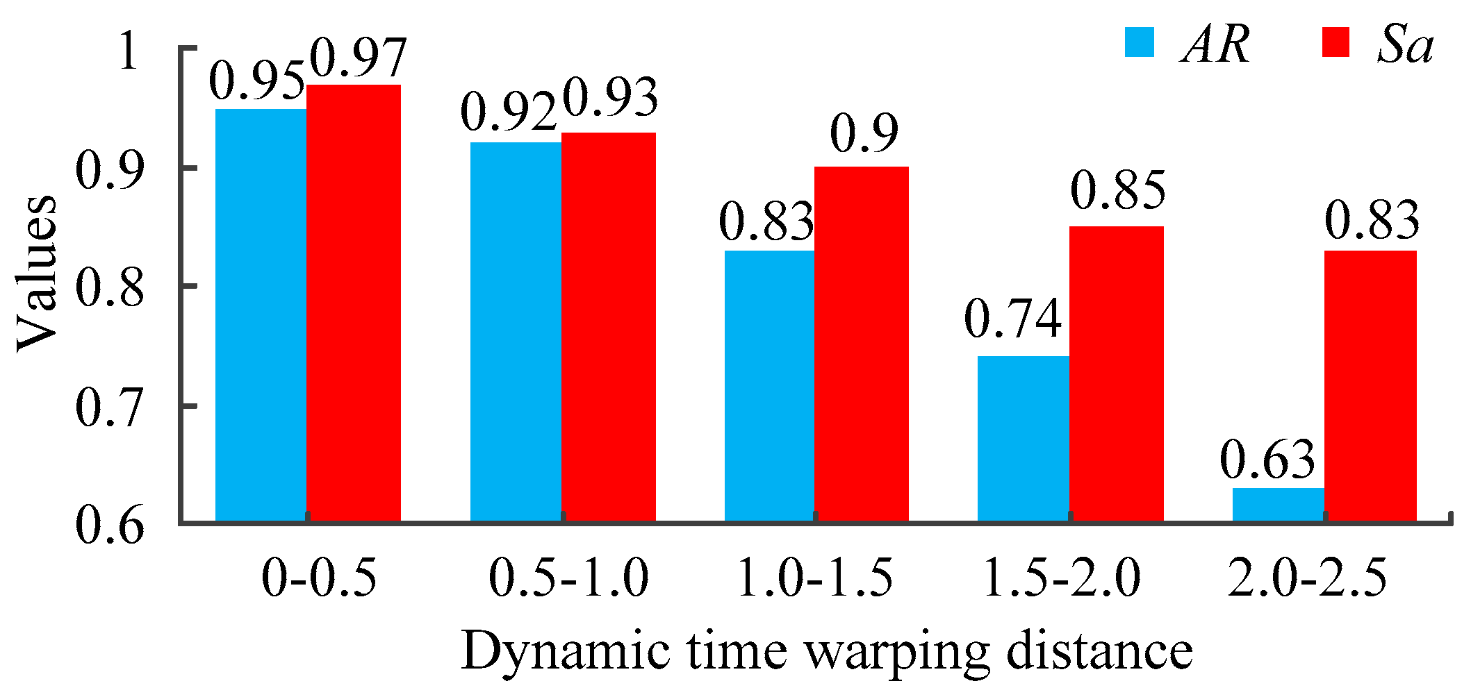
In order to analyze the relationship between the dynamic time warping and the results of time intervals, the schemes of historical cases are applied to the current case. The compression rate is set to 0, and experiments are repeated 50 times respectively. The average accuracy rate and satisfaction of every interval is shown in Figure 11.

Figure 11.
The average accuracy rate and satisfaction of every interval.
As can be seen from Figure 11, the smaller the dynamic time warping is, the higher the satisfaction is. This phenomenon shows that if we apply the scheme of historical cases whose dynamic time warping is smaller into current case, the comprehensive costs will also be smaller. In addition, it can be found that the smaller the dynamic time warping between the historical case and the current case is, the higher the corresponding accuracy rate is. It shows that if the dynamic time warping is smaller, the probability that the scheme of the historical cases is the optimal solution of the current cases is higher.
4.3. The Results of the Static Reconfiguration
1. Compared with traditional algorithms
The active power of each node is taken as the original feature, so the original number of features is 32. According to the symbolic features of historical cases, the classification tree are used to screen several candidate cases for the first time, and adjust the threshold by dichotomy until 50 candidate cases are selected. It assumes that is equal to 10, and the compression ratio is equal to 0. In addition, the optimal control strategy for static reconfiguration is obtained by the enumeration method. The basic steps of the enumeration method are as follows:
Step 1: Close all switches of the distribution network. We assume that the number of rings in the current distribution network is n, and the number of branches that make up the ring network is m.
Step 2: If n branches are disconnected from the m branches, there are a total of species solutions. Among them, some of the solutions should be excluded because there are islands or ring networks in the distribution network.
Step 3: We exclude solutions that do not satisfy the topological constraints, and calculate the power flow of the remaining solutions and the objective function.
Step 4: The optimal control strategy for a case can be obtained according to the value of the objective function.
In order to verify the validity and correctness of the scheme of static reconfiguration based on data-driven model, the proposed method is compared with the traditional methods such as Genetic Algorithm (GA), Particle Swarm Optimization (PSO), Simulated Annealing (SA) and Artificial Bee Colony (ABC). The parameters of the GA are set as follows: The number of chromosomes is 50, and the maximum number of iterations is 50. The probability of crossover is 0.8 and the probability of mutation is 0.2. The parameters of the PSO are set as follows: The number of particles is 50, and the maximum number of iterations is 50. Inertia weight factor is 0.9, learning factors . The parameters of the SA are set as follows: The maximum number of iterations is 20,000 and the temperature coefficient is 0.999. The initial temperature is 1 and the final temperature is 1−9. The parameters of the ABC are set as follows: The number of employed bees and onlooker bees is 20. The number of scout bees is 10 and the number of local searches is 5. The maximum number of iterations is 50. Every method is repeated 50 times respectively and the average result is shown in Table 4.
Table 4.
Results of different methods.
As shown in Table 4, the heuristic algorithms have the potential of finding the global optimal solution in solving the static reconfiguration of distribution network, but it also has the disadvantage of being easily trapped in the local optimal solution. The optimal power loss, the worst power loss and the average power loss of proposed algorithms are smaller than other algorithms. It means that the proposed algorithm can get a better solution than the traditional methods. In terms of computing time, the computation time of the proposed algorithm is far less than the heuristic algorithms and enumeration method. There are three main reasons which result in it. Firstly, the heuristic algorithm searches for the optimal solution by random searching, which consumes a lot of time. Secondly, it needs to satisfy the constraint of topology, and the searching space of heuristic algorithms has a large number of unfeasible solutions, which seriously affects the speed of optimization. Thirdly, the proposed algorithm excludes a large number of historical cases during coarse matching stage, so the number of cases that need to calculate the similarity is very small. In addition, the dimension of features is reduced by principal component analysis, which reduces the complexity of the algorithm. As far as the accuracy rate is concerned, the accuracy rate of the proposed algorithm is higher than that of the other algorithms, which shows that the solution of proposed method has a higher probability as a global optimal solution.
2. The influence of parameters on results
In order to analyze the effect of compression ratio on the results of static reconfiguration, 32 original features are extracted and the dimensions of features are reduced by principal component analysis. It assumes that is equal to 10, and experiments are repeated 50 times respectively. The average accuracy rate of the statistics is shown in Table 5.
Table 5.
The effect of different compression ratio on results.
As shown in Table 5, the computation time is less than 1 s, which can not only be used for offline calculation, but also can meet the requirement of real-time calculation on line. The principal component analysis can reduce the dimensions of the features to a certain extent and reduce the computation time, but it also leads to the reduction of accuracy. Therefore, when the principal component analysis is used, the computation time and accuracy rate should be taken into account simultaneously.
The weight of the feature is determined by using the same weight and the entropy weight respectively to analyze the influence of the weight on the optimization result. It assumes that the compression ratio is equal to 0. The result of the static reconfiguration is shown in Table 6.
Table 6.
The accuracy rate of different methods.
As can be seen from Table 6, compared with the same weight method, the entropy weight method can make full use of the data of each feature to determine the weights so that the accuracy rate of the static reconfiguration is very high.
3. Relationship between dynamic time warping and result of static reconfiguration
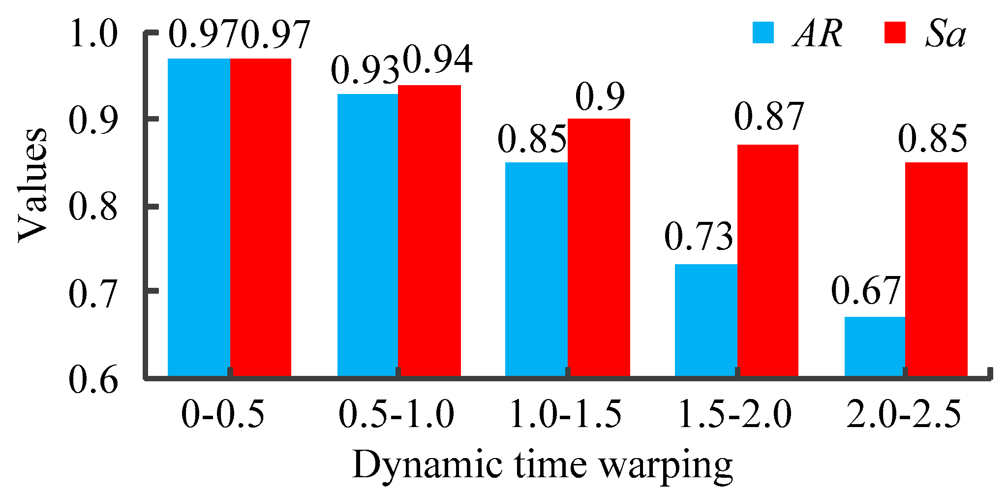
The schemes of historical cases are applied to the current case to analyze the relationship between the dynamic time warping and the results of static reconfiguration. The compression rate is set to 0, and experiments are repeated 50 times respectively. The average accuracy rate and satisfaction of every interval is shown in Figure 12.

Figure 12.
The average accuracy rate and satisfaction of every interval.
As can be seen from Figure 12, if the values of dynamic time warping is smaller than 1, the accuracy rate and satisfaction is high, which means the schemes of historical cases can be applied to current case. The smaller the dynamic time warping is, the higher the satisfaction is. On the contrary, if the values of dynamic time warping is bigger than 1.5, it is not appropriate to apply the schemes of the historical cases to the current case, because this historical case is not very similar to the current case.
5. Conclusions
This paper proposed a dynamic reconfiguration method of distribution network based on Data-driven model from the perspective of data mining, which can make good use of historical cases to guide the operation of current case. Through theoretical analysis and case simulation, following conclusions can be drawn:
- (1)
- The historical cases which are similar to the current case can be selected accurately and quickly by two steps of coarse matching and fine matching.
- (2)
- The principal component analysis can reduce the dimension of features and reduce the computational complexity. However, it will also lose some information of features and make the accuracy rate of the results decrease. Therefore, in order to ensure a sufficient accuracy rate, the compression ratio of features should not be too low.
- (3)
- Entropy weight method can determine the weights according to the information of features and improve the accuracy rate and satisfaction of results.
- (4)
- The smaller the dynamic time warping between the historical case and the current case is, the higher the corresponding accuracy rate is. It shows that if the dynamic time warping is smaller, the probability that the scheme of the historical cases is the optimal solution of the current cases is higher. This probability can be judged by dynamic time warping distance, which is not available in traditional methods.
- (5)
- Compared with the traditional algorithms, optimization results and the computation time of the proposed method are superior to conventional algorithms.
Author Contributions
Funding acquisition, D.Y.; Visualization, D.Y.; Methodology, W.L.; Supervision, W.L.; Writing-original draft, Y.W.; Validation, Y.W.; writing-review & editing, K.Z.; Conceptualization, K.Z.; Investigation, Q.C.; Resources, Q.C.; Formal analysis, D.L.
Funding
This work is supported by the Fundamental Research Funds for the Central Universities (Grant No. 2018XD003).
Acknowledgments
The authors are grateful to Xiang Ren for his suggestions.
Conflicts of Interest
The authors declare no conflict of interest.
References
- Fonseca, A.G.; Tortelli, O.L.; Lourenço, E.M. A reconfiguration analysis tool for distribution networks using fast decoupled power flow. In Proceedings of the 2015 IEEE PES Innovative Smart Grid Technologies Latin America (ISGT LATAM), Montevideo, Uruguay, 5–7 October 2015; pp. 182–187. [Google Scholar]
- Cabezas, A.M.G.; Schmidt, H.P.; Kagan, N.; Gouvea, M.R.; Martin, P.A. Reconfiguration of distribution systems using the newton method in quadratic formulations. IEEE Lat. Am. Trans. 2008, 6, 162–169. [Google Scholar] [CrossRef]
- Fakhry, R.; Abouelseoud, Y.; Negm, E. Mixed-integer quadratically constrained programming with application to distribution networks reconfiguration. In Proceedings of the 2016 Eighteenth International Middle East Power Systems Conference (MEPCON), Cairo, Egypt, 27–29 December 2016; pp. 579–584. [Google Scholar]
- Kumar, K.S.; Rajalakshmi, K.; Karthikeyan, S.P. A modified artificial neural network based distribution system reconfiguration for loss minimization. In Proceedings of the 2014 International Conference on Advances in Electrical Engineering (ICAEE), Vellore, India, 9–11 January 2014; pp. 1–5. [Google Scholar]
- Momoh, J.A.; Caven, A.C. Evaluation of cost benefits analysis for the reconfigured distribution system. In Proceedings of the 2003 IEEE PES Transmission and Distribution Conference and Exposition, Dallas, TX, USA, 7–12 September 2003; pp. 234–241. [Google Scholar]
- Asrari, A.; Lotfifard, S.; Ansari, M. Reconfiguration of smart distribution systems with time varying loads using parallel computing. IEEE Trans. Smart Grid 2016, 7, 2713–2723. [Google Scholar] [CrossRef]
- Sayadi, F.; Esmaeili, S.; Keynia, F. Feeder reconfiguration and capacitor allocation in the presence of non-linear loads using new p-pso algorithm. IET Gen. Transm. Distrib. 2016, 10, 2316–2326. [Google Scholar] [CrossRef]
- Meng, X.; Zhang, L.; Cong, P.; Tang, W.; Zhang, X.; Yang, D. Dynamic reconfiguration of distribution network considering scheduling of dg active power outputs. In Proceedings of the 2014 International Conference on Power System Technology, Chengdu, China, 20–22 October 2014; pp. 1433–1439. [Google Scholar]
- Xu, L.; Cheng, R.; He, Z.; Xiao, J.; Luo, H. Dynamic reconfiguration of distribution network containing distributed generation. In Proceedings of the 2016 9th International Symposium on Computational Intelligence and Design (ISCID), Hangzhou, China, 10–11 December 2016; pp. 3–7. [Google Scholar]
- Yang, H.; Peng, Y.; Xiong, N. Gradual approaching method for distribution network dynamic reconfiguration. In Proceedings of the 2008 Workshop on Power Electronics and Intelligent Transportation System, Guangzhou, China, 2–3 August 2008; pp. 257–260. [Google Scholar]
- Li, Z.; Chen, X.; Yu, K.; Zhao, B.; Liu, H. A novel approach for dynamic reconfiguration of the distribution network via multi-agent system. In Proceedings of the 2008 Third International Conference on Electric Utility Deregulation and Restructuring and Power Technologies, Nanjing, China, 6–9 April 2008; pp. 1305–1311. [Google Scholar]
- Zhou, Z.; Zhao, T.; Zhang, Y.; Su, Y. A data-driven approach to forecasting the distribution of distributed photovoltaic systems. In Proceedings of the 2018 IEEE International Conference on Industrial Technology (ICIT), Lyon, France, 20–22 February 2018; pp. 867–872. [Google Scholar]
- Seyedi, Y.; Karimi, H. Design of networked protection systems for smart distribution grids: A data-driven approach. In Proceedings of the 2017 IEEE Power & Energy Society General Meeting, Chicago, IL, USA, 16–20 July 2017; pp. 1–5. [Google Scholar]
- Chen, X.; Wu, W.; Zhang, B.; Lin, C. Data-driven dg capacity assessment method for active distribution networks. IEEE Trans. Power Syst. 2017, 32, 3946–3957. [Google Scholar] [CrossRef]
- Hasna, O.L.; Potolea, R. Time series, a taxonomy based survey. In Proceedings of the 2017 13th IEEE International Conference on Intelligent Computer Communication and Processing (ICCP), Cluj-Napoca, Romania, 7–9 September 2017; pp. 231–238. [Google Scholar]
- Ji, C.; Liu, S.; Yang, C.; Wu, L.; Pan, L.; Meng, X. A piecewise linear representation method based on importance data points for time series data. In Proceedings of the 2016 IEEE 20th International Conference on Computer Supported Cooperative Work in Design (CSCWD), Nanchang, China, 4–6 May 2016; pp. 111–116. [Google Scholar]
- Burke, D.J.; Malley, M.J.O. A study of principal component analysis applied to spatially distributed wind power. IEEE Trans. Power Syst. 2011, 26, 2084–2092. [Google Scholar] [CrossRef]
- Deladreue, S.; Brouaye, F.; Bastard, P.; Peligry, L. Using two multivariate methods for line congestion study in transmission systems under uncertainty. IEEE Trans. Power Syst. 2003, 18, 353–358. [Google Scholar] [CrossRef]
- Gajera, V.; Gupta, R.; Jana, P.K. An effective multi-objective task scheduling algorithm using min-max normalization in cloud computing. In Proceedings of the 2016 2nd International Conference on Applied and Theoretical Computing and Communication Technology (iCATccT), Bangalore, India, 21–23 July 2016; pp. 812–816. [Google Scholar]
- Cao, X.; Dong, S.; Wu, Z.; Jing, Y. A data-driven hybrid optimization model for short-term residential load forecasting. In Proceedings of the 2015 IEEE International Conference on Computer and Information Technology, Liverpool, UK, 26–28 October 2015; pp. 283–287. [Google Scholar]
- Li, X.; Gu, Y.; Huang, P.C.; Liu, D.; Liang, L. Downsampling of time-series data for approximated dynamic time warping on nonvolatile memories. In Proceedings of the 2017 IEEE 6th Non-Volatile Memory Systems and Applications Symposium (NVMSA), Hsinchu, Taiwan, 16–18 August 2017; pp. 1–6. [Google Scholar]
- Chen, Q.; Hu, G.; Gu, F.; Xiang, P. Learning optimal warping window size of dtw for time series classification. In Proceedings of the 2012 11th International Conference on Information Science, Signal Processing and their Applications (ISSPA), Montreal, QC, Canada, 2–5 July 2012; pp. 1272–1277. [Google Scholar]
- Tin, T.T.; Hien, N.T.; Vinh, V.T. Measuring similarity between vehicle speed records using dynamic time warping. In Proceedings of the 2015 Seventh International Conference on Knowledge and Systems Engineering (KSE), Ho Chi Minh City, Vietnam, 8–10 October 2015; pp. 168–173. [Google Scholar]
- Baran, M.E.; Wu, F.F. Network reconfiguration in distribution systems for loss reduction and load balancing. IEEE Trans. Power Deliv. 1989, 4, 1401–1407. [Google Scholar] [CrossRef]


© 2018 by the authors. Licensee MDPI, Basel, Switzerland. This article is an open access article distributed under the terms and conditions of the Creative Commons Attribution (CC BY) license (http://creativecommons.org/licenses/by/4.0/).