Influence of Blade Leading-Edge Shape on Cavitation in a Centrifugal Pump Impeller

Abstract

Cavitation is an important issue in pumps and usually starts on the blade leading-edge. For fixed blades with constant rotational speeds and specific flow rates, the incident angle, which is between the flow direction and the blade installing direction, on the blade leading-edge plays the key role in the cavitation process. The leading-edge shape is crucial on the local flow separation, pressure distribution, and cavitation. Hence, the influence of the leading-edge shape on cavitation has been studied in the current work in a centrifugal pump impeller. The blunt, sharp, ellipse and round leading-edge cases were compared using numerical simulation and verified by experimental data. Results show different features of cavitation. The round and ellipse leading-edge impellers have higher inception cavitation coefficient. It was caused by the sudden pressure drop on leading-edge arc or elliptical arc. The sharp and blunt leading-edge impellers have a wide flow-separation region on leading-edge with a wide low-pressure region. This is because of the sudden turn in geometry on the leading-edge corner. Cavitation grew quickly after inception and caused rapid head-drop in the sharp and blunt leading-edge impellers. Results suggest the critical cavitation performance is dominated by the leading-edge low-pressure area while the inception cavitation is mostly affected by the minimum pressure value on the leading-edge. The critical cavitation performance can be evaluated by checking the leading-edge low-pressure area. The inception cavitation can be evaluated by checking the minimum pressure value on the leading-edge. These strategies can be used in the further leading-edge designs.

1. Introduction

Cavitation is a liquid-gas phase change which happens below the saturation pressure [1]. Reynolds explained the cavitation phenomenon in 1873. In the past 140 years, people tried to understand cavitation including its physical phenomena, bubble dynamics and engineering influences. There are two essential factors of cavitation which are the nucleation sites and the sufficient low pressure [2]. In hydraulic machinery, the two factors are available. Firstly, natural liquid contains a certain amount of dissolved gas nuclei at specific environment [3]. Secondly, pressure varies in the flow field which may drop below the saturation pressure [4]. Usually, cavitation has bad hydrodynamic influences including noise [5], vibration [6], material damage [7] and performance drop [8]. This is why researchers and engineers usually try to reduce or eliminate cavitation.

In pump impellers, cavitation incepts on the blade leading-edge which is the lowest pressure site. Pressure drops here because of the incoming flow striking and following separation [9]. At a high cavitation number condition, cavitation performs as traveling individual bubbles [10]. If cavitation number decreases, the scale of cavitation would increase and performs as fixed sheet type [11] at low incidence angles and vortexed cloud type at high incidence angles [12]. As the lowest pressure region, the pressure distribution on blade leading-edge is important for cavitation inception and development. The pressure distribution is influenced by leading-edge geometry [13]. For a fixed blade at a constant rotation speed and a specific flow rate, the incidence angle is a certain value [14]. Thus, how thickness increases along blade meanline will be crucial for the local pressure field and cavitation.

How to decide the leading-edge shape is a puzzle in pump impeller design. In the traditional design methods of pumps, the blade angles, wrap angles, blade numbers and other parameters can be decided mathematically or empirically [15,16,17]. However, the determination of leading-edge shape has no certain method. If cavitation margin is large, the leading-edge shape can be designed simply as an arc or elliptical arc. If cavitation margin is small, the design of leading-edge shape should consider the local pressure drop condition. There is an argument in pump design theories. Traditional design method prefer thinner leading-edge thickness for design condition. Some handbooks believe a thinner thickness would reduce blade expelling and generate lower-velocity and higher-pressure [18]. Some other analyses proved that a thinner thickness makes weaker separation, smaller low-pressure region and later critical cavitation at design-load [19,20]. Recently, researchers tried thicker streamlined leading-edge shape on large-discharge pump units. Flow analysis showed that the thicker streamlined leading-edge shape has gentler local pressure drop which delayed the inception cavitation [21,22]. There are some researches to compare the flow around different leading-edge shape and explain the relationship between flow separation and pressure distribution [23,24,25]. Also, there are already studies to compare the cavitation behavior under different leading-edge shapes [26,27]. However, the influence of leading-edge shape on the local flow and the mechanism of separation-induced cavitation under impeller rotating effects are still not clear. The design differences for delaying inception cavitation and critical cavitation are quite different. Hence, further detailed analyses on this topic are necessary.

To identify the design requirements for the leading edge shape, the cavitating flow in a centrifugal impeller with 4 different leading-edge shapes were studied. The blunt, sharp, ellipse and round leading-edge shapes were discussed at a specific rotation speed and flow rate. The interference of incidence angle factor was excluded. The influence of blade leading-edge shape on the cavitation in a centrifugal impeller can be focused on. It will help the design and determination of the blade leading-edge shape for delay the inception cavitation or critical cavitation.

2. Numerical Method

In this study, the computational fluid dynamics (CFD) method was used for the flow field simulation. The Reynolds-Averaged Navier-Stokes (RANS) equations were used which were closed by Shear Stress Transport (SST) k-ω model [28,29]. The k and ω equations are:

$$\frac{\partial \left(\rho k\right)}{\partial t}+\frac{\partial \left(\rho u_{i}k\right)}{\partial x_i}=P-\frac{\rho k^{3/2}}{l_{k-\omega }}+\frac{\partial }{\partial x_i}\left[\left(\mu +{\sigma }_k{\mu }_t\right)\frac{\partial k}{\partial x_i}\right]$$

(1)

$$\frac{\partial \left(\rho \omega \right)}{\partial t}+\frac{\partial \left(\rho u_i\omega \right)}{\partial x_i}=C_{\omega }P-\beta \rho {\omega }^2+\frac{\partial }{\partial x_i}\left[\left({\mu }_l+{\sigma }_{\omega }{\mu }_t\right)\frac{\partial \omega }{\partial x_i}\right]+2\left(1-F_1\right)\frac{\rho {\sigma }_{\omega 2}}{\omega }\frac{\partial k}{\partial x_i}\frac{\partial \omega }{\partial x_i}$$

(2)

where t, denote the time, ρ the density, u the velocity and x the coordinate. P is the production term, μ is the dynamic viscosity, μ_t is the turbulent eddy viscosity, σ are the model constants, C_ω is the coefficient of the production term, and l_k-ω is the turbulence scale. F₁ is the zonal mixture function which is used to combine the standard k-ε model [30] and Wilcox’s k-ω model [31]. The k-ω formulation is used in the inner parts of the boundary layer with the k-ε formulation used in the free-stream. Combining the advantages of k-ε and k-ω models, it can evaluate both the strong shear flow and the near-wall boundary layer flow well, so that it is a good choice for the pump impeller internal flow case. Hence, the SST k-ω model can be used as a low-Re model and avoids the over-sensitivity for inlet free-stream cases.

Considering the rotation/curvature effect on turbulence flow, the Spalart-Shur correction to SST k-ω model was applied for a better prediction [32]. This correction adds the correction term f_r1 as a multiplier on the production term P_k:

$$P_k\to f_{r1}{P}_k$$

(3)

where f_r1 is given empirically with specific limiters as:

$$f_{r1}=\max \left[0,1+C_s\left(f_r^{*}\right)\right]$$

(4)

$$f_r^{*}=\max \left[\min \left(f_{rot},1.25\right),0\right]$$

(5)

$$f_{rot}=\left(1+C_{r1}\right)\frac{2r^{*}}{1+r^{*}}\left[1-C_{r3}{\tan }^{-1}\left(C_{r2}\widehat{r}\right)\right]-C_{r1}$$

(6)

where C_s is an empirical scale factor which allows control of the correction strength level for specific flow cases. The constants C_r1, C_r2 and C_r3 are equal to 1.0, 2.0 and 1.0. The remaining functions are defined as:

$$r^{*}=\frac{S}{\Omega }$$

(7)

$$\Omega =\sqrt{2{\Omega }_{ij}{\Omega }_{ij}}$$

(8)

$$\widehat{r}=\frac{2{\Omega }_{ik}{S}_{jk}}{\Omega B^3}\left[\frac{D{S}_{ij}}{Dt}+\left({\epsilon }_{imn}{S}_{jn}+{\epsilon }_{jmn}{S}_{in}\right){\Omega }_m^{rot}\right]$$

(9)

$$B^2=\max \left(S^2,0.09{\omega }^2\right)$$

(10)

where Ω^rot is the rotation rate of the reference frame and the term DS_ij/D_t represents the Lagrangian derivative of the strain rate tensor. The empirical scale factor C_s was tuned and validated for a better adaptability.

3. Case and Setup

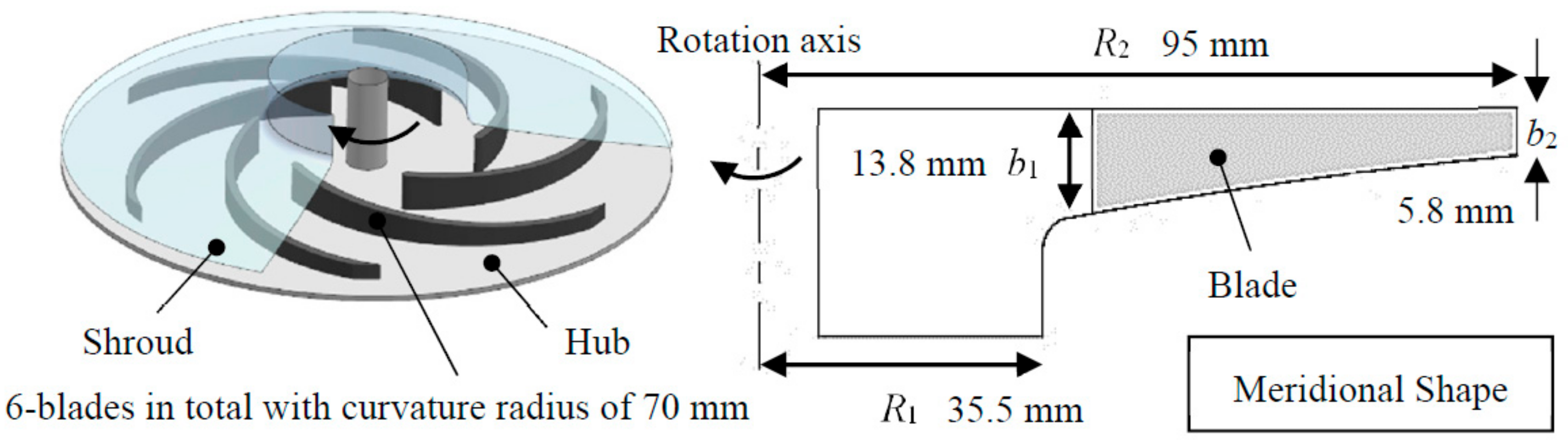
3.1. Impeller Geometry

The centrifugal pump impeller tested by Pedersen et al. [33,34] with sufficient experimental works were used as the studied object. This is a typical impeller flow case which have been validated by many researchers [35,36,37]. Figure 1 shows the schematic map of this impeller. The rotating speed is 725 rpm and the design mass flow rate is 3.06 kg/s.

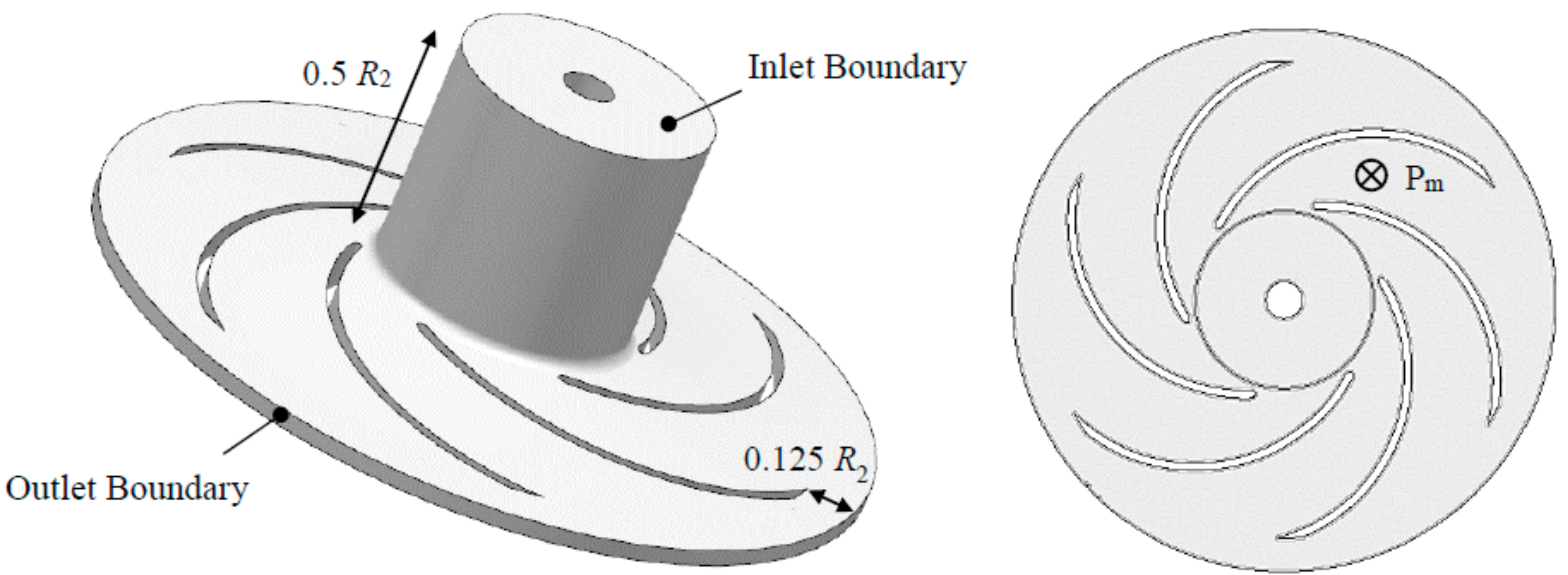
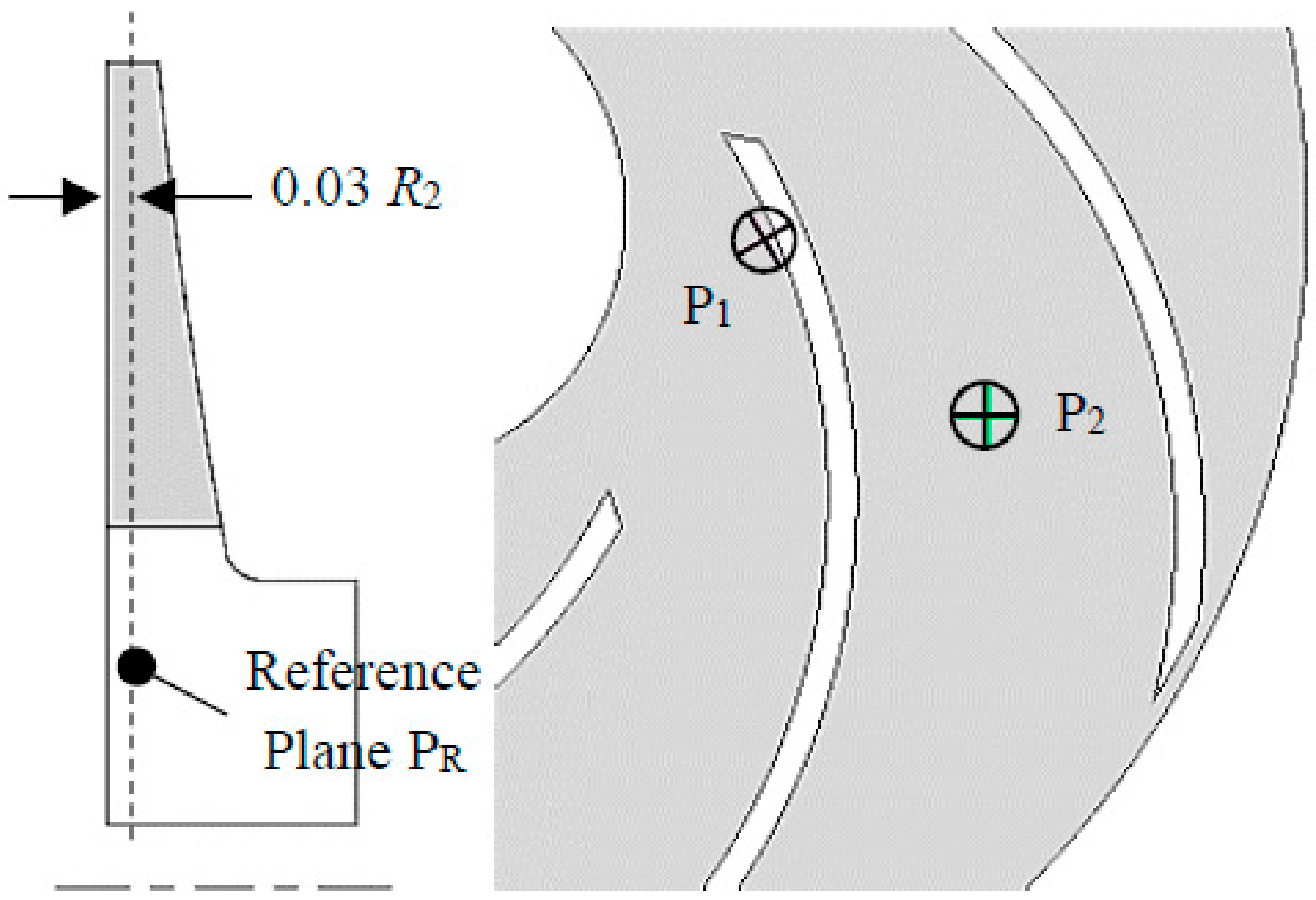
3.2. Domain Modeling and Meshing

The flow domain was modeled with 0.5 R₂ long inflow section before blades and 0.125 R₂ long outflow section after blades. It was meshed by hexahedral elements using commercial code ICEMCFD in ANSYS (v12.0, Pittsburgh, PA, USA). A mesh independence check was conducted before the final mesh was selected using turbulent kinetic energy k_2D at the monitoring point P_m indicated in Figure 2.

Table 1. Mesh independence check details.

No.	Mesh	Nodes	k2D on Pm [m2/s2]	Residual Against Mesh No. 1
1	Very Coarse	41308	1.5861 × 10−2	-
2	Coarse	82528	1.5383 × 10−2	3.014%
3	Medium	159836	1.5130 × 10−2	1.645%
4	Fine	323332	1.5082 × 10−2	0.317%
5	Very Fine	602024	1.5083 × 10−2	0.007%

shows the mesh independence check details. The fine scheme with 323,332 nodes in total was chosen when the k_2D residual on P_m becomes less than 1%. Prism layers were set off-wall for a better simulation of the flow in the near-wall region. Five prism layers were put off-wall with the growth rate of 1.2. The y⁺ value was controlled within 30–300 which is suitable for SST k-ω model with automatic wall-functions.

3.3. Computational Setup

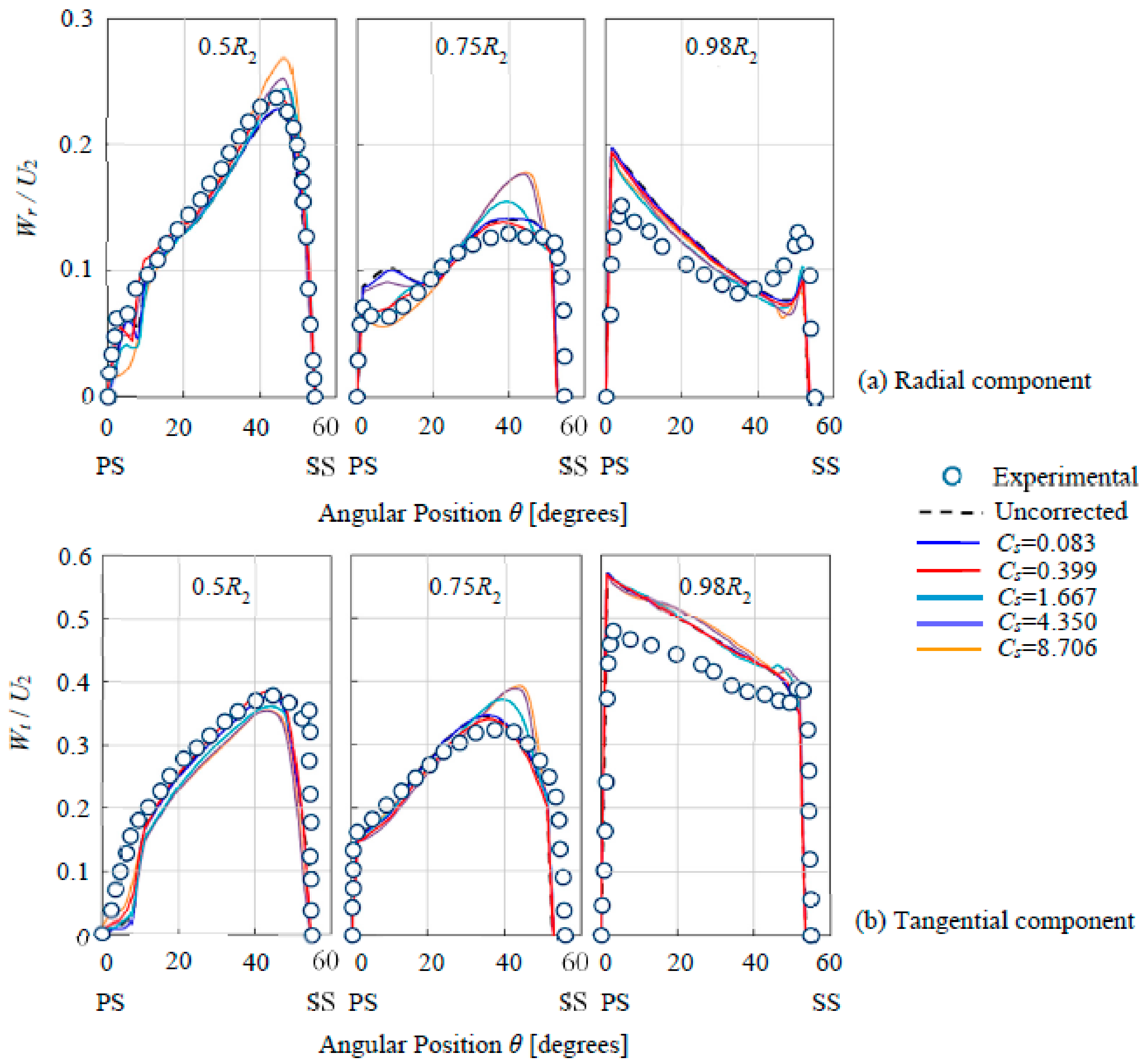
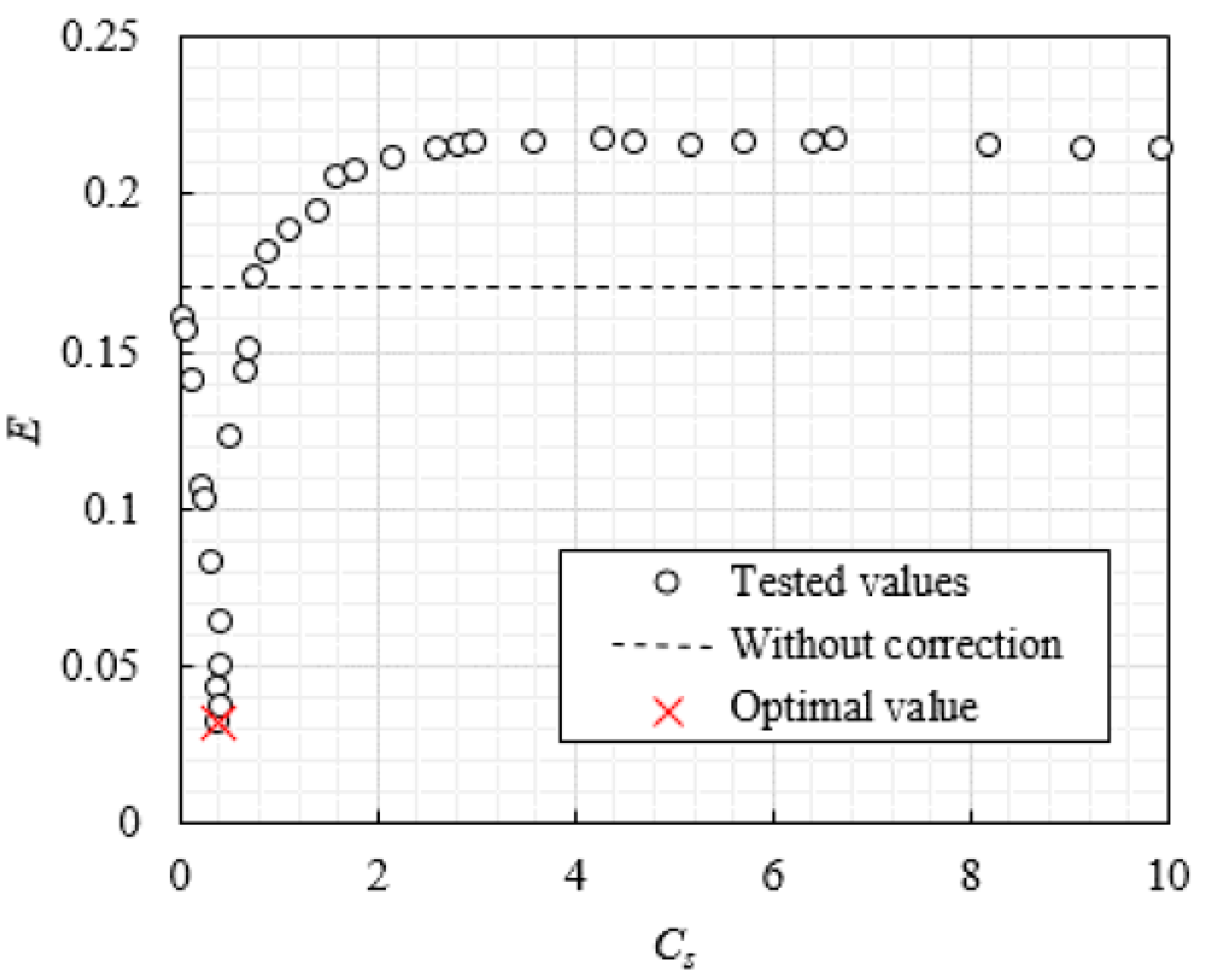
Based on the domain shown in Figure 2, the CFD computations were set as follows based on the commercial code CFX in ANSYS (v12.0, Pittsburgh, PA, USA). Firstly, the rotational speed of the domain was set as 725 rpm. Secondly, the boundary conditions were set. A velocity inlet boundary was given at the impeller inflow. The pressure on this boundary follows the Neumann condition. A static pressure boundary was given at the outflow. The pressure value was set as 0 Pa and the velocity follows the Neumann condition. No-slip walls were given on the impeller hub, shroud and blades. Thirdly, the fluid medium was given as water at 20 °C and the reference pressure was set as 1 atm. For cavitating flow, two parameters were set as:

$$C_p=\frac{p-p_{\infty }}{\rho gH}-\frac{V_{\infty }^2}{2gH}$$

(11)

$$C_{\sigma }=\frac{p_{\infty }-p_v}{\rho gH}+\frac{V_{\infty }^2}{2gH}$$

(12)

where C_p is the dimensionless pressure coefficient and C_σ is the dimensionless cavitation coefficient. p_∞ and V_∞ are respectively the reference pressure and velocity. The reference position for p_∞ and V_∞ are on the inlet boundary. p_v is the saturation pressure which is 2300 Pa here. g is the gravitational acceleration. H is the head of impeller. For the mass transfer simulation in cavitation, the Zwart-Gerber-Belamri model was used [38].

4. Model Tuning

4.1. Tuning Process

There was a model tuning work to make the simulation more reliable. Based on the SST k-ω model and rotation/curvature correction, the value of the empirical scale factor C_s was discussed. Two points P₁ and P₂ were set on the reference plane P_R as the indicator of model tuning as shown in Figure 3. Parameter E based on the turbulent kinetic energy k_2D on P₁ and P₂ was used for checking:

$$E=\left[\mathrm{abs}\left(k_{2D}^{com1}-k_{2D}^{exp1}\right)+\mathrm{abs}\left(k_{2D}^{com2}-k_{2D}^{exp2}\right)+\mathrm{abs}\left(\overline{k_{2D}^{com}}-\overline{k_{2D}^{exp}}\right)\right]/3$$

(13)

where the superscript com denotes the computational data, exp denotes the experimental data, 1 denotes the data on P₁ and 2 denotes the data on P₂. The average value considered the data on P₁ and P₂. It can be considered that smaller E is, more accurate the simulation is.

The C_s values from 0 to 10 were randomly tested as shown in Figure 4. The E value of uncorrected model was about 0.17. When C_s was between 2 to 10, E was over 0.2. E started to decrease when C_s decreased from 2. E became below 0.17 (uncorrected) when C_s < 0.78. A valley was found around C_s = 0.4. E increased again when C_s decreased from about 0.4 to 0. By fitting and interpolating, the optimal C_s value which had the smallest E was found on C_s = 0.399.

4.2. Verification of Tuning

After tuning, the verification of the tuned model was conducted by comparing with the experimental data [33]. Figure 5 is the comparison of k_2D contours on reference plane P_R. 5 typical C_s situations were discussed including 0.083, 0.399 (optimal), 1.667, 4.350 and 8.706. The two situations that C_s = 4.350 and 8.706 were completely incorrect without capturing the high-k_2D region on blade leading-edge on suction side. The situations that C_s = 0.083, 0.399 and 1.667 found the high-k_2D region on blade leading-edge on suction side. However, the intensity in this region was too strong for C_s = 0.083 and too weak for C_s = 1.667. Among them, the situation C_s = 0.399 correctly captured the experimental k_2D pattern. The flow at the key places including the suction side of leading-edge, pressure side of leading-edge and the suction side of trailing-edge were all accurately described. Figure 6 also compares the distribution of velocities on P_R along the tangential direction θ where W_r is the radial component of the relative velocity W and W_t is the tangential component of the relative velocity W. The situations that C_s = 0.083, 0.399 and 1.667 found the similar velocity characters with the experimental data by Particle Image Velocimetry (PIV) measurement [33]. There are some differences at the location R = 0.98 R₂. The differences might be caused by the domain simplification that the computation domain did not include the space-vane after impeller. However, the variation tendency is the same among the numerical and experimental data. It means that the simulation is somehow accurate especially for comparative study. Thus, the optimal C_s value of 0.399 can be used for the simulation.

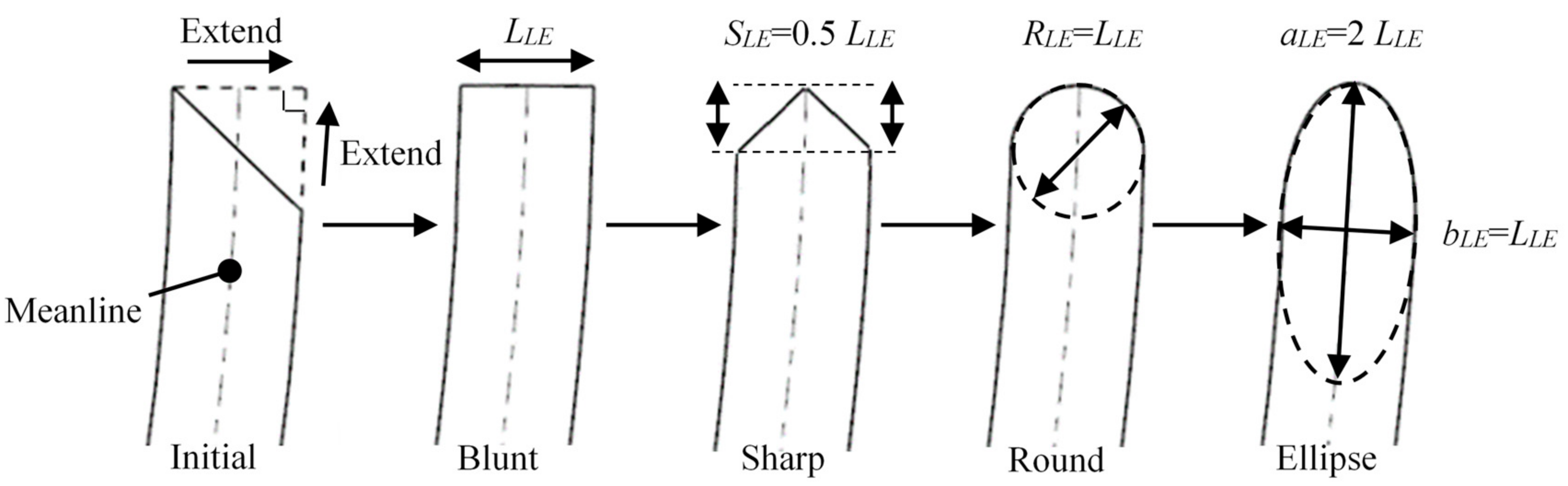
5. Leading-Edge Reshaping

Figure 7 shows the blade leading-edge “reshape” that is the re-modeling after the changes in the blade leading-edge geometry. Based on the initial shape, the initial leading-edge geometry was extended along the meanline direction and perpendicular to the meanline direction. After extension, the blunt leading-edge whose width was L_LE was made. Then, the two sides of the blunt leading-edge by S_LE which was equal to 0.5 L_LE was cut and made the sharp leading-edge. Based on the blunt leading-edge, the round leading-edge whose radius was R_LE = L_LE was made. Finally, an ellipse leading-edge was made whose long axis was a_LE = 2 L_LE and short axis b_LE was b_LE = L_LE. The four new leading-edge shapes were comparatively studied mainly on their cavitation behaviors. The influence of leading-edge shape was discussed in detail.

6. Comparative Analyses

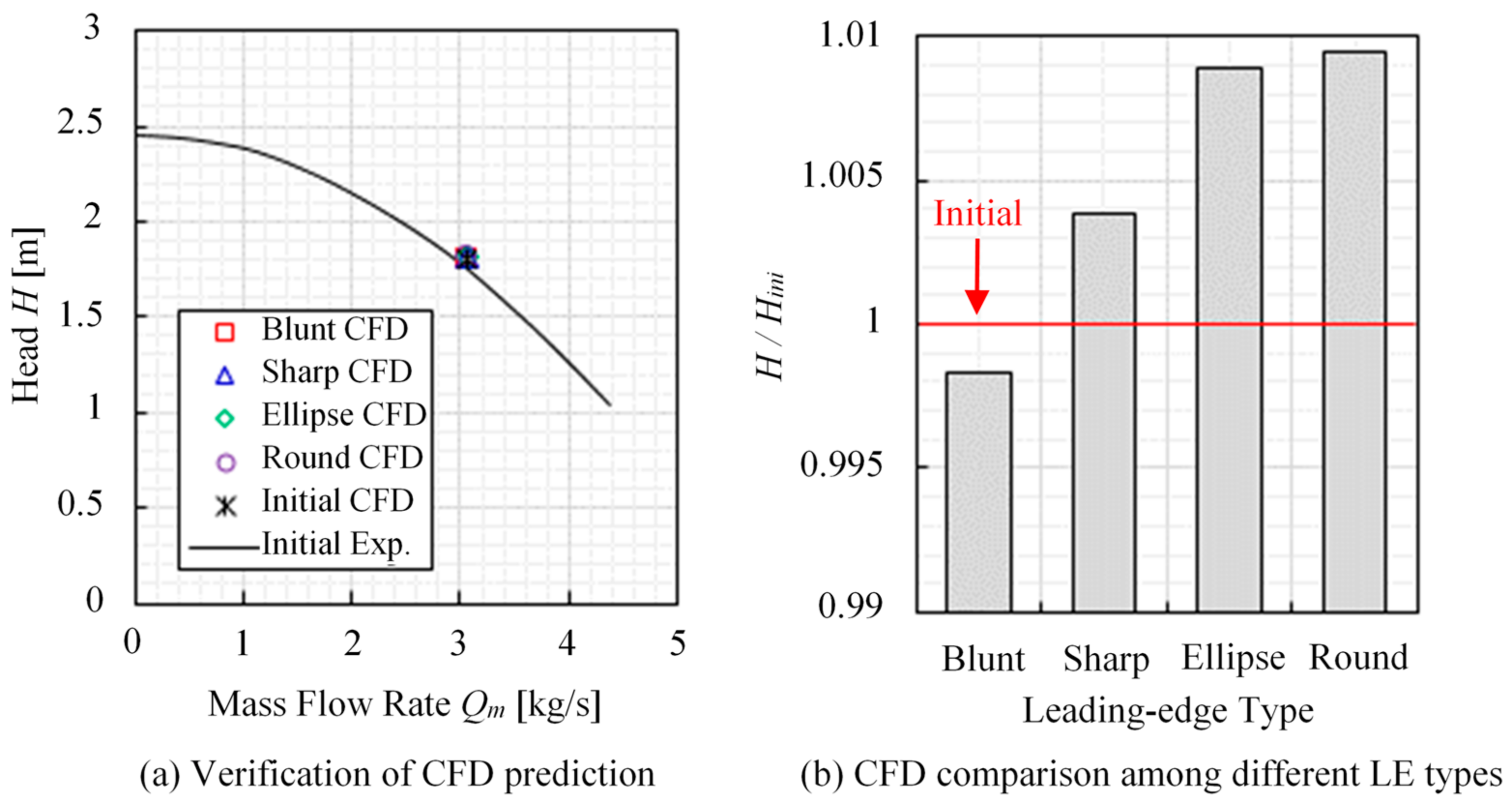
6.1. Pump Performance

The head performance of the different leading-edge types was compared. H is the impeller head which can be calculated as:

H = (p_in − p_out)/ρg

(14)

where p_in and p_out are the static pressure at impeller inlet and outlet.

In Figure 8a, the CFD predicted H values were compared with the experimental H [33]. The CFD predicted H value of the initial impeller was similar to the experimental H value. It showed that the CFD prediction of the performance was accurate. Figure 8b shows the comparison of the CFD predicted H of the 4 new reshaped leading-edge types against the initial leading-edge impeller’s head H_ini. The blunt leading-edge impeller has the lowest H and the round leading-edge impeller has the highest H. There were only small differences of H (≈1%) after the leading-edge reshaping. Compared with the initial leading-edge impeller, the sharp, ellipse and round leading-edge impellers has a slightly higher H.

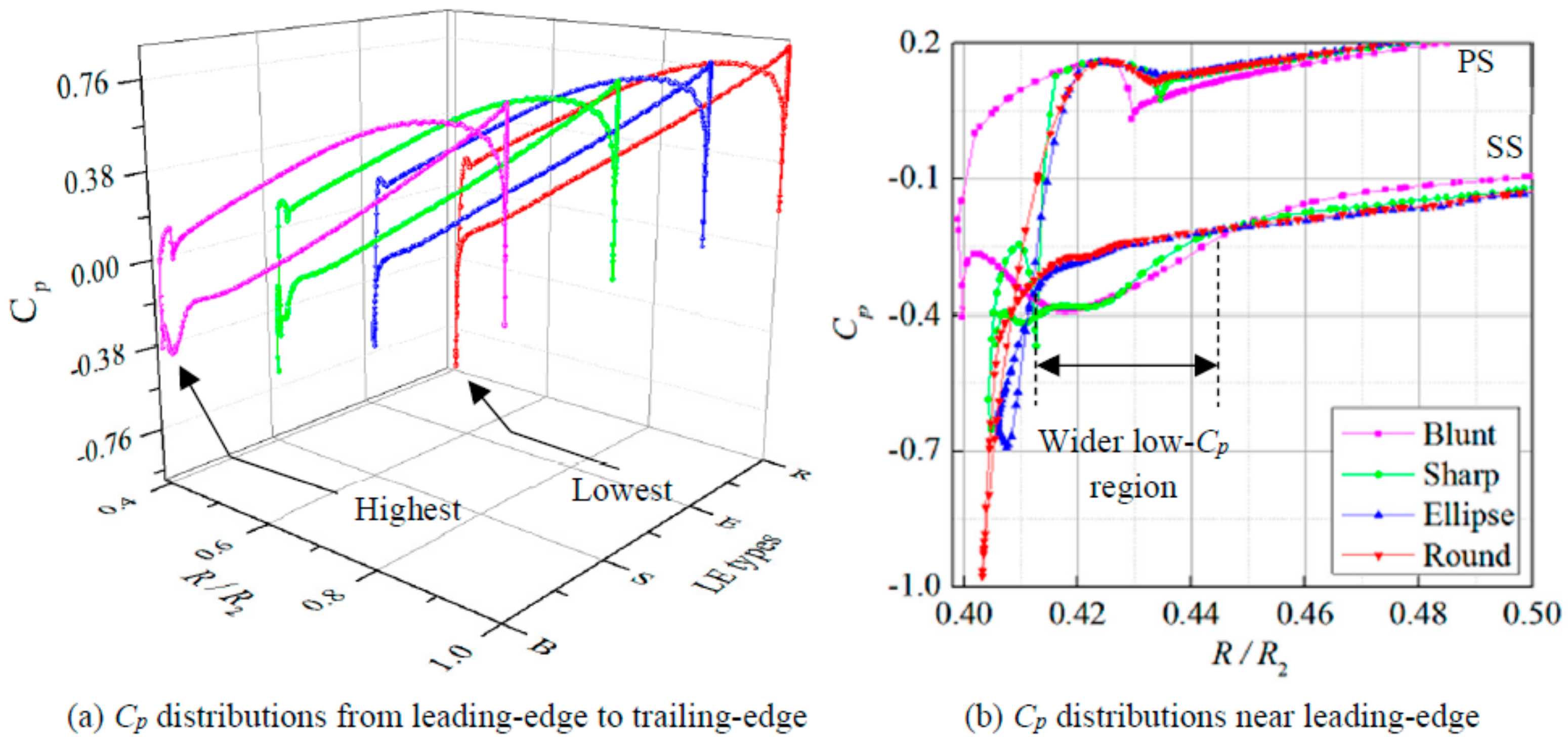
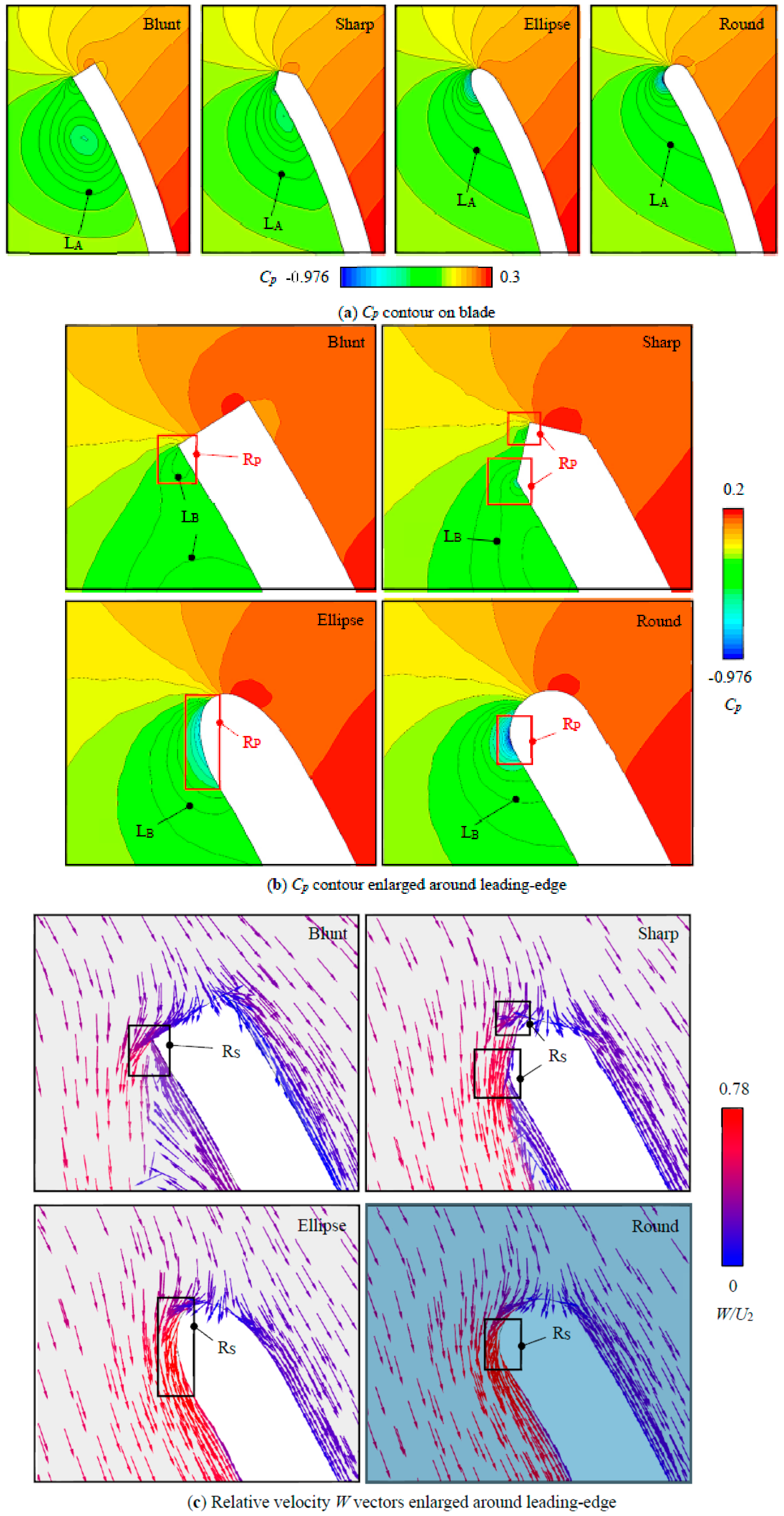
6.2. Pressure Distribution

According to Equation (11), the pressure coefficient C_p distributions on blade were analyzed. Figure 9 shows the distribution of C_p on a single blade on the reference plane P_R shown in Figure 3. The blunt, sharp, ellipse and round leading-edge impellers were compared. The variation of pressure has three stages. Firstly, it increased on the leading-edge on the pressure side and decreased on the leading-edge on the suction side due to the local flow striking and separation. Secondly, pressure increased along the direction from leading-edge to trailing-edge because of the impeller work ability. Thirdly, pressure dropped on the trailing-edge on the suction side due to the flow separation.

Compared among the 4 types of leading-edge, it was found that the amplitude of leading-edge pressure drop which is also the minimum pressure point on blade. The blunt leading-edge impeller had the highest minimum pressure coefficient C_pmin which was about −0.408. The round leading-edge impeller had the lowest C_pmin which was about −0.976. The C_pmin values on the sharp leading-edge and ellipse leading-edge were similar which were about −0.653 and −0.692, respectively. Based on Equations (11) and (12), C_p will be equal to C_σ when p is equal to p_v. When the minimum pressure p_min drops to the saturation pressure p_v, cavitation incepts. Thus, for cavitation inception, here is:

−C_pmin = C_σi

(15)

where C_pmin is the minimum value of C_p, C_σi is the inception cavitation number. Hence, cavitation is easier to happen on the round leading-edge blade and harder on the blunt leading-edge impeller. Behind the leading-edge position, the low pressure increased to a high level immediately on the ellipse and round leading-edge impellers. However, there were a wider low-C_p region on the sharp and blunt leading-edge impellers. If the pressure in this region drops below p_v, there will be large-scale cavitation. Thus, it is necessary to know the development of cavitation after inception.

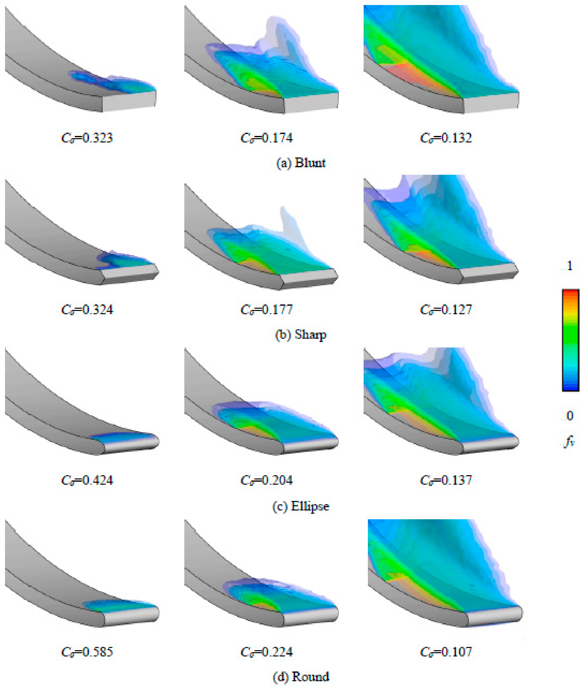
6.3. Development of Cavitation Scale

Figure 10 shows variation of the cavitation vapor volume fraction V_vap/V_imp where V_vap is the vapor volume and V_imp is the impeller domain volume. During the decreasing of C_σ, the blunt leading-edge impeller had the latest cavitation inception but the quickest development of vapor volume. V_vap/V_imp of blunt leading-edge impeller increased to about 0.087 when C_σ decreased from 0.408 to 0.135. On the contrary, the round leading-edge impeller had the earliest cavitation inception but the slow development of vapor volume. V_vap/V_imp of round leading-edge impeller increased to about 0.066 when C_σ decreased from 0.976 to 0.110. The V_vap/V_imp variation rate of ellipse and sharp leading-edge impeller were between the round and blunt leading-edge impeller.

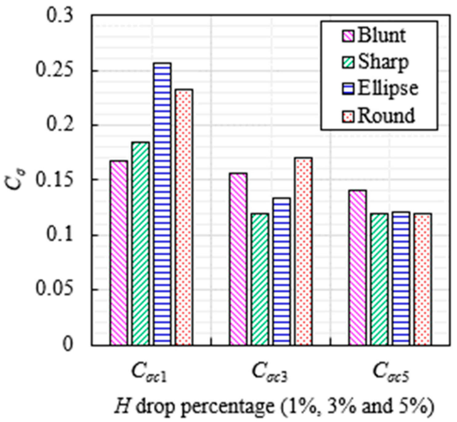
6.4. Cavitation-Induced Performance Drop

In pumps and other hydraulic turbomachineries, critical cavitation is very important. It was defined when the pump performance drops by some specific percentage (for example 0.5%, 1% or 3%) against the cavitation-free performance. The performance can be the head H or the efficiency η. In this case, the drop of head H on the 4 new leading-edge types of impellers were also checked.

Figure 11 shows the variation of head H against the cavitation-free head H_free. During the decreasing of C_σ, H was relatively stable at first, gently dropped when about C_σ < 0.3, suddenly dropped when about C_σ < 0.2. Compared among the 4 impellers, the head drop happened always in about C_σ = 0.1~0.3 even their inception cavitation coefficient C_σi were completely different. Fitting and interpolating from the data shown in Figure 11, it was found that the critical cavitation coefficient C_σc of 1%, 3% and 5% H drop which were denoted as C_σc1, C_σc3 and C_σc5. The values of C_σc1, C_σc3 and C_σc5 are comparatively shown in Figure 12. During the decreasing of C_σ, H drops by 1% following the sequence that ellipse, round, sharp and blunt. It means that the ellipse and round leading-edge impellers have larger cavitation at first. Then, H drops by 3% following the sequence that round, blunt, ellipse and sharp. The round leading-edge impeller was still under the cavitation influence on its head. However, the H-drop became quicker in the blunt leading-edge impeller than in the other 3 impellers. Finally, H drops by 5% earlier in the blunt leading-edge impeller than in the other 3 impellers. It means that the cavitation grew rapidly in the blunt leading-edge impeller. It can be also observed that the C_σc3 and C_σc5 value of sharp leading-edge impeller were similar. It means that the cavitation in the sharp leading-edge impeller grew suddenly in this range.

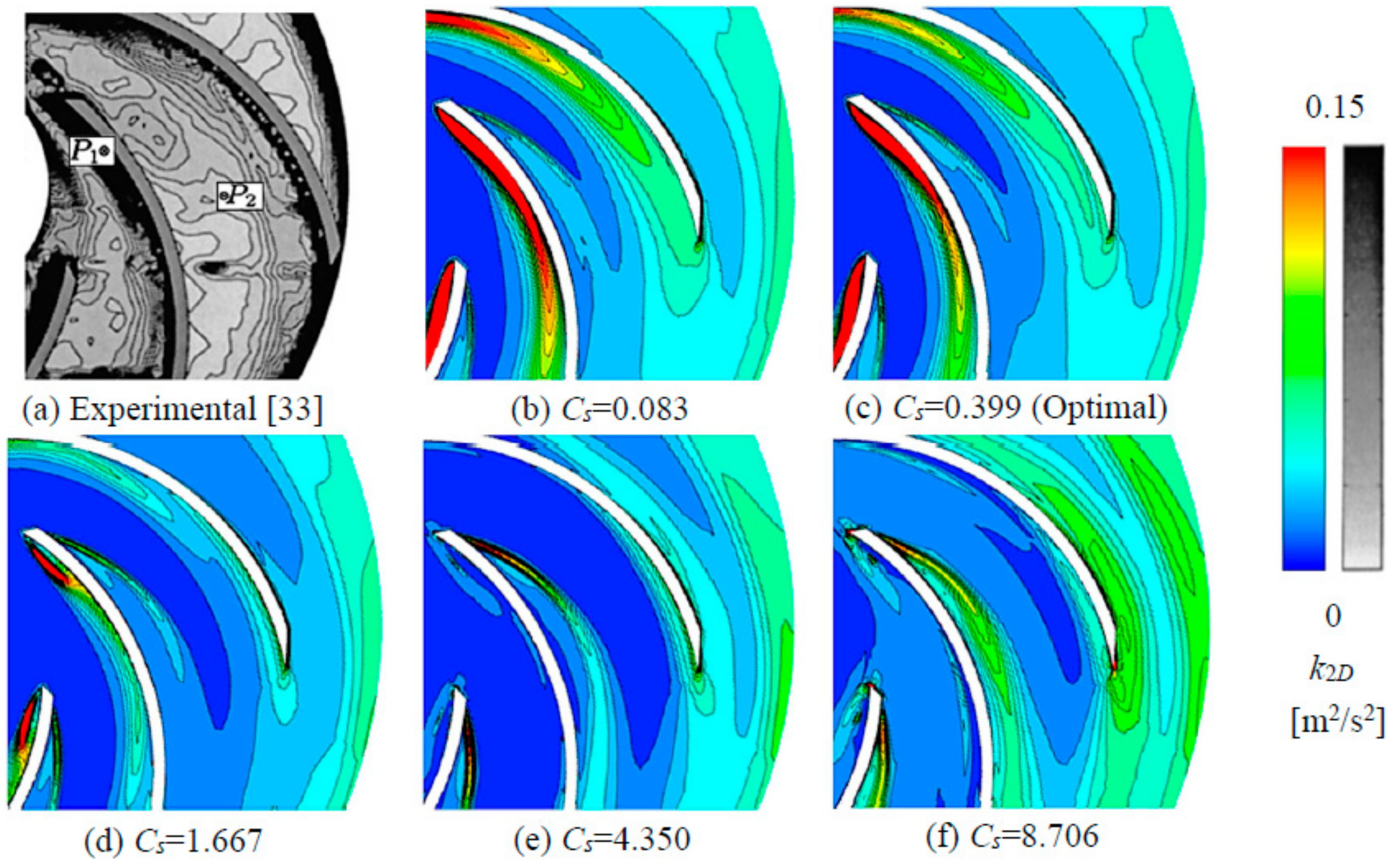
6.5. Flow Field Analyses

To understand the difference of cavitation behavior caused by leading-edge shape, the flow field was analyzed especially around the blade leading-edge. Figure 13a shows the C_p contour on blade. As an example, the isoline L_A of C_p = −0.253 was specifically drawn which represented a low pressure region. On the round leading-edge, there was a sudden pressure drop region where C_p < −0.5. On the other 3 types of leading-edges, the amplitudes of C_p drop were not so large. However, the region C_p < −0.253 of blunt leading-edge was the biggest. On the contrary, the region C_p < −0.253 of round leading-edge was the smallest. The C_p contour was in accordance with the pressure distribution shown in Figure 9. This is why cavitation incepted early on the round leading-edge and why cavitation grew quickly on the blunt leading-edge.

Figure 13b,c comparatively shows the C_p contour and relative velocity W vectors enlarged around leading-edge. The local low pressure region was denoted as R_P and the local separation region was denoted as R_S. On the blunt leading-edge, there was a separation region on the left corner (blade suction side) and induced low pressure. On the sharp leading-edge, there were two corners on the leading-edge. Separations and induced low pressure regions occurred on these two corners. On the ellipse and round leading-edge, there were no corners but continually variation of geometry. Separation and low pressure region occurred where geometry varied relatively quickly. Relative velocity W were on a high level in the separation region.

Generally, the leading-edge shape has strong influence on the local flow separation, pressure distribution and cavitation. For the blunt and sharp leading-edges, blade geometry changed immediately on the corners. Fluid kept its direction behind the corner and generated a large backflow area on the suction side. It induced a wide low pressure region where C_p did not dropped so suddenly. For the continually variated geometry of round and ellipse leading-edge, the low pressure regions were narrow and the pressure drops were sudden. Comparatively speaking, the round leading-edge geometry (arc) varied quicker than the ellipse leading-edge geometry (elliptical arc) along the flow direction. Thus, the round leading-edge has the highest C_p drop amplitude and the earliest cavitation inception during the C_σ decreasing.

Figure 14 shows the shape variation of cavitation vapor on blade. When C_σ was larger than 0.3, the cavity scale was small. There was a difference among the 4 types of leading-edge impellers. On the blunt and sharp leading-edges, the cavity separated from the blade surface. On the round leading-edge, the cavity trail also slightly separated. On the ellipse leading-edge, the cavity attached on the blade surface as the sheet cavitation style. This difference was because of the intensity of flow separation behind leading-edge. When C_σ was within 0.17~0.23, the cavity scale became bigger. The cavity was separated on the blunt and sharp leading-edges and still attached on the ellipse and round leading-edges. Finally, when C_σ was smaller than 0.14, the cavity scale became very large. Separation was found on all the types of leading-edges.

7. Conclusions

According to the studies above, conclusions can be drawn as follows:

(1) The Spalart-Shur rotation/curvature correction was used in this centrifugal impeller flow case to solve the system-rotation and streamline-curved flow. At the design-load, the empirical turbulence scale factor C_s was tuned by a broad-searching. The optimal value of C_s was about 0.399. Compared with the experimental data, the optimal case got a correct pattern of the turbulence kinetic energy in impeller. The predictions of the velocity components were also more accurate. Improvements of CFD simulation can be found after the rotation/curvature correction and tuning.

(2) Local flow striking and separation was found on the blade leading-edge. A local sudden pressure drop happened on the leading-edge due to separation. As a pump, pressure increased from leading-edge to trailing-edge under the design-load condition. The low-pressure side of blade overlapped the leading-edge pressure drop. Thus, the lowest pressure point located in the leading-edge separation region. With the decreasing of cavitation coefficient C_σ, cavitation incepted in the lowest pressure region. If C_σ decreased further, the cavity scale became stronger and somehow flow-blocking. The pump head and other performances would be impacted. The cavitation vapor volume could be very large by 4~8% of the impeller volume when achieving the 1% head drop.

(3) The leading-edge shape strongly impacted the local separation, pressure drop and cavitation. On the blunt and sharp leading-edges, geometry varied immediately at the local corner. Flow separated due to the immediately turned geometry with a wide low-pressure region. On the ellipse and round leading-edges, geometry varied smoothly. Flow separation happened where the geometry changed relatively quicker. By comparison, the separation region on the ellipse and round leading-edges was smaller in size but larger in pressure drop amplitude. Among the 4 types of leading-edges, the round leading-edge has the highest pressure drop amplitude and the largest inception cavitation coefficient C_σi. On the contrary, the blunt leading-edge has the lowest pressure drop amplitude and the smallest C_σi. However, because of the wider separation and low-pressure region, cavitation grew quickly on the blunt and sharp leading-edges. The critical cavitation coefficient by 5% head drop C_σc5 was the much larger on the blunt leading-edge than on the other 3 leading-edges. When designing the leading-edge shape, the critical cavitation performance can be evaluated by checking the leading-edge low-pressure area. Otherwise, it is necessary to check the minimum pressure value on the leading-edge while caring about the inception cavitation and try to eliminate the cavitation at all.

References

1. Franc, J.P.; Michel, J.M. Fundamentals of Cavitation; Springer: Heidelberg, Germany, 2010. [Google Scholar]
2. Brennen, C.E. Cavitation and Bubble Dynamics; Oxford University Press: New York, NY, USA, 1995. [Google Scholar]
3. Henry, W. Experiments on the quantity of gases absorbed by water, at different temperatures, and under different pressures. Philos. Trans. R. Soc. Lond. 1803, 93, 29–274. [Google Scholar] [CrossRef]
4. Arndt, R.E.A. Cavitation in fluid machinery and hydraulic structures. Annu. Rev. Fluid Mech. 1981, 13, 273–326. [Google Scholar] [CrossRef]
5. Wu, Q.; Huang, B.; Wang, G.; Cao, S.; Zhu, M. Numerical modelling of unsteady cavitation and induced noise around a marine propeller. Ocean Eng. 2018, 160, 143–155. [Google Scholar] [CrossRef]
6. Valentín, D.; Presas, A.; Egusquiza, M.; Valero, C.; Egusquiza, E. Transmission of high frequency vibrations in rotating systems. Application to cavitation detection in hydraulic turbines. Appl. Sci. 2018, 8, 451. [Google Scholar] [CrossRef]
7. Mouvanal, S.; Chatterjee, D.; Bakshi, S.; Burkhardt, A.; Mohr, V. Numerical prediction of potential cavitation erosion in fuel injectors. Int. J. Multiph. Flow 2018, 104, 113–124. [Google Scholar] [CrossRef]
8. Hao, Y.; Tan, L. Symmetrical and unsymmetrical tip clearances on cavitation performance and radial force of a mixed flow pump as turbine at pump mode. Renew. Energy 2018, 127, 368–376. [Google Scholar] [CrossRef]
9. Hirschi, R.; Dupont, P.; Avellan, F.; Favre, J.N.; Guelich, J.F.; Parkinson, E. Centrifugal pump performance drop due to leading edge cavitation: Numerical predictions compared with model tests. J. Fluids Eng. Trans. ASME 1998, 120, 705–711. [Google Scholar] [CrossRef]
10. Guennoun, F.; Farhat, M.; Ait Bouziad, Y.; Avellan, F.; Pereira, F. Experimental investigation of a particular traveling bubble cavitation. In Proceedings of the 5th International Symposium on Cavitation, Osaka, Japan, 1–4 November 2003. [Google Scholar]
11. Dijkers, R.J.; Fumex, B.; de Woerd, J.O.; Kruyt, N.P.; Hoeijmakers, H.W. Prediction of sheet cavitation in a centrifugal pump impeller with the three-dimensional potential-flow model. In Proceedings of the 2005 ASME Fluids Engineering Division Summer Meeting and Exhibition, Houston, TX, USA, 1 January 2005. [Google Scholar]
12. Shi, L.; Zhang, D.; Zhao, R.; Shi, W.; BPM, B.V. Visualized observations of trajectory and dynamics of unsteady tip cloud cavitating vortices in axial flow pump. J. Fluid Sci. Technol. 2017, 12, JFST0007. [Google Scholar] [CrossRef]
13. Epps, B.; Víquez, O.; Chryssostomidis, C. A method for propeller blade optimization and cavitation inception mitigation. J. Ship Prod. Des. 2015, 31, 88–99. [Google Scholar] [CrossRef]
14. Tuzson, J. Centrifugal Pump Design; Wiley-Interscience: Hoboken, NJ, USA, 2000. [Google Scholar]
15. Han, X.; Kang, Y.; Li, D.; Zhao, W. Impeller Optimized Design of the Centrifugal Pump: A Numerical and Experimental Investigation. Energies 2018, 11, 1444. [Google Scholar] [CrossRef]
16. Xie, H.; Song, M.; Liu, X.; Yang, B.; Gu, C. Research on the Simplified Design of a Centrifugal Compressor Impeller Based on Meridional Plane Modification. Appl. Sci. 2018, 8, 1339. [Google Scholar] [CrossRef]
17. Li, P.; Han, Z.; Jia, X.; Mei, Z.; Han, X. Analysis of the Effects of Blade Installation Angle and Blade Number on Radial-Inflow Turbine Stator Flow Performance. Energies 2018, 11, 2258. [Google Scholar] [CrossRef]
18. Guan, X. Modern Pumps Theory and Design; China Astronautics Publishing House: Beijing, China, 2011. [Google Scholar]
19. Wei, W.; Pengbo, L.; Xiaofang, W. Blade optimal design and cavitation investigation based on state equation model of mixed-flow pump. J. Dalian Univ. Technol. 2013, 53, 189–194. [Google Scholar]
20. Ruan, H.; Luo, X.; Liao, W.; Zhao, Y. Effects of low pressure edge thickness on cavitation performance and strength for pump-turbine. Trans. Chin. Soc. Agric. Eng. 2015, 31, 32–39. [Google Scholar]
21. Tao, R.; Xiao, R.; Wang, F.; Liu, W. Cavitation behavior study in the pump mode of a reversible pump-turbine. Renew. Energy 2018, 125, 655–667. [Google Scholar] [CrossRef]
22. IH, S.; JW, A. Influence of the leading edge shape of a 2-dimensional hydrofoil on cavitation characteristics. J. Soc. Nav. Arch. Korea 2000, 37, 60–66. [Google Scholar]
23. Kang, C.; Yang, M.; Wu, G.; Liu, H. Cavitation analysis near blade leading edge of an axial-flow pump. In Proceedings of the 2009 International Conference on Measuring Technology and Mechatronics Automation, Zhangjiajie, China, 11 April 2009. [Google Scholar]
24. Hofmann, M.; Stoffel, B.; Friedrichs, J.; Kosyna, G. Similarities and geometrical effects on rotating cavitation in two scaled centrifugal pumps. In Proceedings of the 4th International Symposium on Cavitation, Pasadena, CA, USA, 20–23 June 2001. [Google Scholar]
25. Christopher, S.; Kumaraswamy, S. Identification of critical net positive suction head from noise and vibration in a radial flow pump for different leading edge profiles of the vane. J. Fluids Eng. Trans. ASME 2013, 135, 121301. [Google Scholar] [CrossRef]
26. Balasubramanian, R.; Sabini, E.; Bradshaw, S. Influence of impeller leading edge profiles on cavitation and suction performance. In Proceedings of the 27th International Pump Users Symposium, Houston, TX, USA, 12–15 September 2011. [Google Scholar]
27. Bakir, F.; Kouidri, S.; Noguera, R.; Rey, R. Experimental analysis of an axial inducer influence of the shape of the blade leading edge on the performances in cavitating regime. J. Fluids Eng. Trans. ASME 2003, 143, 691–696. [Google Scholar] [CrossRef]
28. Menter, F.R. Zonal two equation k-turbulence models for aerodynamic flows. AIAA Pap. 1993, 7, 2906. [Google Scholar]
29. Menter, F.R. Ten years of experience with the SST turbulence model. Turbul. Heat Mass Transf. 2003, 4, 625–632. [Google Scholar]
30. Launder, B.E.; Sharma, B.I. Application of the energy-dissipation model of turbulence to the calculation of flow near a spinning disc. Lett. Heat Mass Transf. 1974, 1, 131–137. [Google Scholar] [CrossRef]
31. Wilcox, D.C. Re-assessment of the scale-determining equation for advanced turbulence models. AIAA J. 1988, 26, 1299–1310. [Google Scholar] [CrossRef]
32. Spalart, P.R.; Shur, M. On the sensitization of turbulence models to rotation and curvature. Aerosp. Sci. Technol. 1997, 1, 297–302. [Google Scholar] [CrossRef]
33. Pedersen, N.; Jacobsen, C.B.; Larsen, P.S. Flow in a centrifugal pump impeller at design and off-design conditions-part I: Particle image velocimetry (PIV) and laser Doppler velocimetry (LDV) measurements. J. Fluids Eng. Trans. ASME 2003, 125, 61–72. [Google Scholar] [CrossRef]
34. Byskov, R.K.; Jacobsen, C.B.; Pedersen, N. Flow in a centrifugal pump impeller at design and off-design conditions-part II: Large eddy simulations. J. Fluids Eng. Trans. ASME 2003, 125, 73–83. [Google Scholar] [CrossRef]
35. Zhang, W.; Ma, Z.; Yu, Y.C.; Chen, H.X. Applied new rotation correction k-ω SST model for turbulence simulation of centrifugal impeller in the rotating frame of reference. J. Hydrodyn. Ser. B 2010, 22, 404–407. [Google Scholar] [CrossRef]
36. Huang, X.; Liu, Z.; Yang, W. Comparative study of SGS models for simulating the flow in a centrifugal-pump impeller using single passage. Eng. Comput. 2015, 32, 2120–2135. [Google Scholar] [CrossRef]
37. Yang, Z.; Wang, F.; Zhou, P. Evaluation of subgrid-scale models in large-eddy simulations of turbulent flow in a centrifugal pump impeller. Chin. J. Mech. Eng. 2012, 25, 911–918. [Google Scholar] [CrossRef]
38. Zwart, P.J.; Gerber, A.G.; Belamri, T. A two-phase flow model for predicting cavitation dynamics. In Proceedings of the 5th International Conference on Multiphase Flow, Yokohama, Japan, 30 May–4 June 2004. [Google Scholar]
Figure 1. Schematic map of centrifugal impeller with its geometric parameters.
Energies 11 02588 g001
Figure 2. Flow domain of the centrifugal impeller and the point for mesh independence check.
Energies 11 02588 g002
Figure 3. Reference plane and points for model tuning.
Energies 11 02588 g003
Figure 4. Model tuning and optimal selection.
Energies 11 02588 g004
Figure 5. Comparison of k2D contours.
Energies 11 02588 g005
Figure 6. Comparison of velocity distributions along tangential direction.
Energies 11 02588 g006
Figure 7. Four new types of leading-edge shape.
Energies 11 02588 g007
Figure 8. Head performance of impeller.
Energies 11 02588 g008
Figure 9. Pressure distribution and variation on a single blade, B: blunt, S: sharp, E: ellipse, R: round, PS: pressure side, SS: suction side.
Energies 11 02588 g009
Figure 10. Variation of the cavitation vapor volume fraction in impeller.
Energies 11 02588 g010
Figure 11. Variation of the impeller head.
Energies 11 02588 g011
Figure 12. Comparison of critical cavitation coefficients.
Energies 11 02588 g012
Figure 13. Flow field around leading-edge, isoline LA: Cp = −0.253, isoline LB: Cp = −0.329.
Energies 11 02588 g013
Figure 14. Variation of cavitation vapor shape on blade.
Energies 11 02588 g014