Article

Study and Application of Intelligent Sliding Mode Control for Voltage Source Inverters

Department of Electrical Engineering, I-Shou University, No.1, Sec. 1, Syuecheng Rd., Dashu District, Kaohsiung City 84001, Taiwan
Energies 2018, 11(10), 2544; https://doi.org/10.3390/en11102544
Submission received: 30 July 2018 / Revised: 18 September 2018 / Accepted: 23 September 2018 / Published: 24 September 2018
(This article belongs to the Special Issue Power Electronics in DC-Microgrid Systems)

Abstract

:
In this paper, an intelligent sliding mode controlled voltage source inverter (VSI) is developed to achieve not only quick transient behavior, but satisfactory steady-state response. The presented approach combines the respective merits of a nonsingular fast terminal attractor (NFTA) as well as an adaptive neuro-fuzzy inference system (ANFIS). The NFTA allows no singularity and error states to be converged to the equilibrium within a finite time, while conventional sliding mode control (SMC) leads to long-term (infinite) convergent behavior. However, there is the likelihood of chattering or steady-state error occurring in NFTA due to the overestimation or underestimation of system uncertainty bound. The ANFIS with accurate estimation and the ease of implementation is employed in NFTA for suppressing the chatter or steady-state error so as to improve the system’s robustness against uncertain disturbances. Simulation results display that this described approach yields low distorted output wave shapes and quick transience in the presence of capacitor input rectifier loading as well as abrupt connection of linear loads. Experimental results conducted on a 1 kW VSI prototype with control algorithm implementation in Texas Instruments DSP (digital signal processor) support the theoretic analysis and reaffirm the robust performance of the developed VSI. Because the proposed VSI yields remarkable benefits over conventional terminal attractor VSIs on the basis of computational quickness and unsophisticated realization, the presented approach is a noteworthy referral to the designers of correlated VSI applications in future, such as DC (direct current) microgrids and AC (alternating current) microgrids, or even hybrid AC/DC microgrids.

1. Introduction

Distributed energy resources (DERs)-based microgrids can yield electricity to the grid and once the power grid goes out unexpectedly. Such microgrids assure the reliability of electricity supply with the presence of sensitive loads [1,2,3]. The DERs require power electronic interfaces for the connection of the microgrid. Generally, we can group the microgrids into two types, i.e., DC microgrids and AC microgrids. Owing to better compatibility, higher efficiency and robust stability, the DC microgrids have gained more and more research interest. In a DC microgrid, voltage source inverters can be adopted as an interface between the DC grid and typical AC loading. The inverter works in two different modes. One is island mode, where the inverter can be regarded as a voltage source. It can afford the devices with sine voltage, and pulse width modulated control can be used in this mode. The other operation mode allows the delivery of the current to the grid, and another control scheme can be adopted like hysteresis current control. Using reference voltage tracking techniques, the voltage source inverter (VSI) can control the voltage quality of the distribution networks [4,5]. Diverse methodologies can be found in publications, namely the H-infinity approach, the deadbeat technique and the fractional order repetitive controller [6,7,8]. However, there is a compromise between the transient response and the steady-state response. Sliding mode control (SMC) offers insensitivity against parametric uncertainties and external disturbances [9,10,11]. The SMC has been attempted to design VSI [12,13,14,15,16,17,18,19,20,21]. The grid-tied inverter controlled by the fixed switching frequency SMC is developed. A good steady-state response can be obtained, but chatter and poor transience exist [12,13]. The ingenious combination of a proportional-resonant and a SMC is suggested to improve the system response of the single-phase inverter. Even if the transient behavior of system performance is effectively improved, the presented algorithm leads to steady-state errors [14,15]. A control method based on the multi-slope sliding surface is also employed for single-phase inverter design. The transient and steady state behavior is compromising while feeding nonlinear loads [16,17]. Using a stable switching manifold to enhance the robustness of a grid-connected inverter has been reported. The state trajectory cannot touch the predetermined sliding manifold in a fast finite time, thus displaying output-voltage distortion [18,19]. Additionally, an improved sliding mode controller for a photovoltaic inverter is presented by [20,21]. Although such an improved methodology has shown fast transience and satisfactory steady-state response, the problem of the chattering still appears around the sliding manifold. It is important to heed that the long convergence time and the chattering phenomenon exist in the above-mentioned conventional SMCs.
During the past few years, terminal attractors (TAs) have attracted growing interest for application in different areas [22,23]. TAs can provide finite time tracking while still preserving the robustness of the conventional SMC [24,25]. Unfortunately, TAs still produce the difficulties in singularity and chattering. The singularity may cause the system states to converge to zero in infinite time. For the sake of suppressing the singularity, the nonsingular fast terminal attractor (NFTA) is introduced in this paper. The NFTA makes tracking error on the sliding surface converge to zero within a finite time, thus obtaining closed-loop stability. For practical applications, unmodeled dynamic uncertainty and parametric plant perturbation, and external disturbances are not so easy to estimate beforehand. If the uncertain boundary conditions are somewhat big or small, a large amount of chattering or steady-state error happens, losing the existence and invariance of the sliding mode. Former works have recommended high-gain feedback to reject perturbations resulting from boundary uncertainties. Employing large constant gain is easy to implement, but there is unpopular chattering or steady-state error occurring in the plant system [26,27]. Many studies have found that the chattering or steady-state error can be attenuated by the use of the observer method or hybrid control strategy [28,29,30,31,32,33,34,35]. A low-cost microcontroller under hybrid control has been presented. The proposed controller effectively reduces the chattering, but there is a steady-state error in response to sudden load disturbance [28,29]. The improved observer due to higher accuracy and stronger robustness is also introduced into sliding mode design for a servo system. Though good steady-state behavior can be seen, the output waveform shows a slow dynamic response during the transient stage [30,31]. To withstand parameter variations and load interferences, a sliding control with an adaptive law combined with an expert semantic description is used to control a grid-connected inverter. The resulting waveforms display a fast transient characteristic, however a large amount of chattering still exists in this presented method [32,33]. By the application of a typical microgrid, the developed system with the association of fuzzy and SMC can obtain improved performance in steady-state and transient responses. Unfortunately, such a methodology is complex and needs heavy calculation [34,35]. To address the problem of the chattering or steady-state error, an adaptive neuro-fuzzy inference system (ANFIS) incorporating both neural networks and fuzzy logic principles is employed in this paper. [36,37]. A neural network is a kind of supervised learning algorithm, which uses a historical dataset to forecast future values. In fuzzy logic, the control signal is produced from the firing of the rule base. Using this hybrid-learning algorithm, the difference between demanded and real outputs is minimized, therefore weakening the chattering when the estimation value exceeds the uncertain system boundary, or reducing steady-state error when the estimation value falls short of the uncertain system boundary [38,39,40]. With the association of ANFIS and NFTA, the proposed approach can yield a VSI feedback control with many advantages, such as finite-time fast convergence without inflicting any singularity, fast dynamic response, low THD (total harmonic distortion), chattering reduction and less steady-state error in the presence of transient loading and steady-state loading. Comparison and discussion of the results in simulation and experiment are provided to corroborate the applicability and feasibility of the proposed approach.

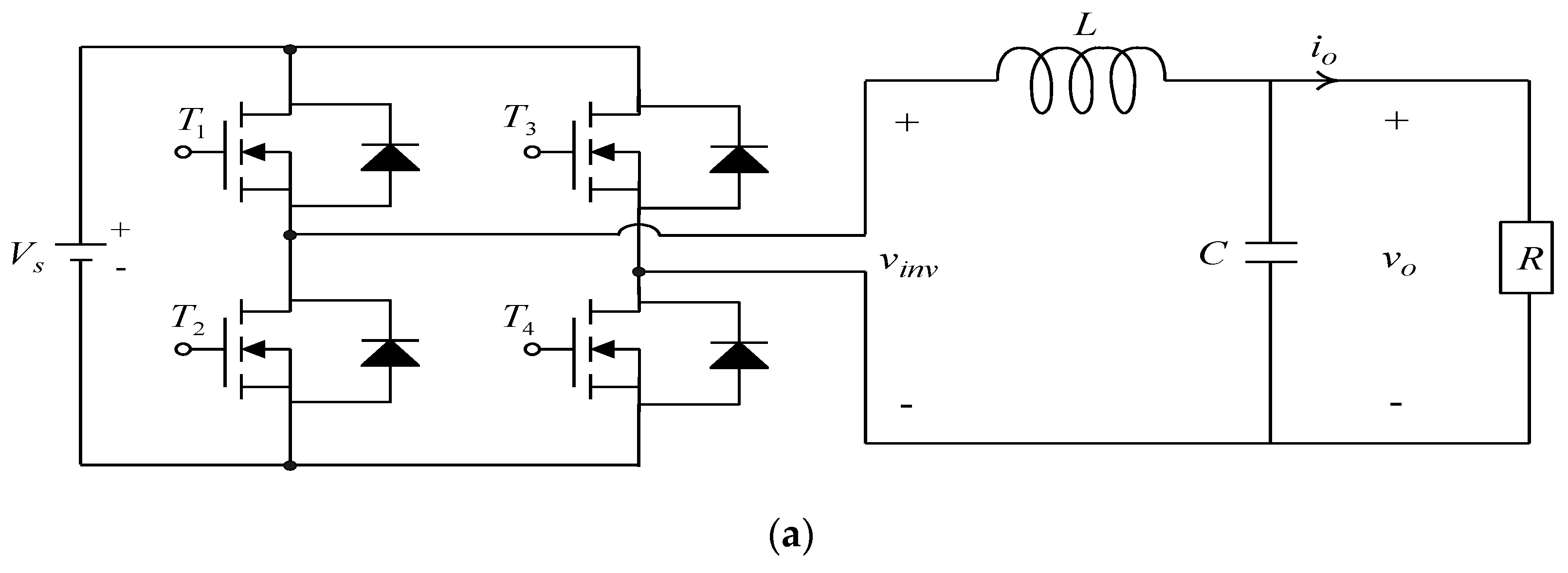
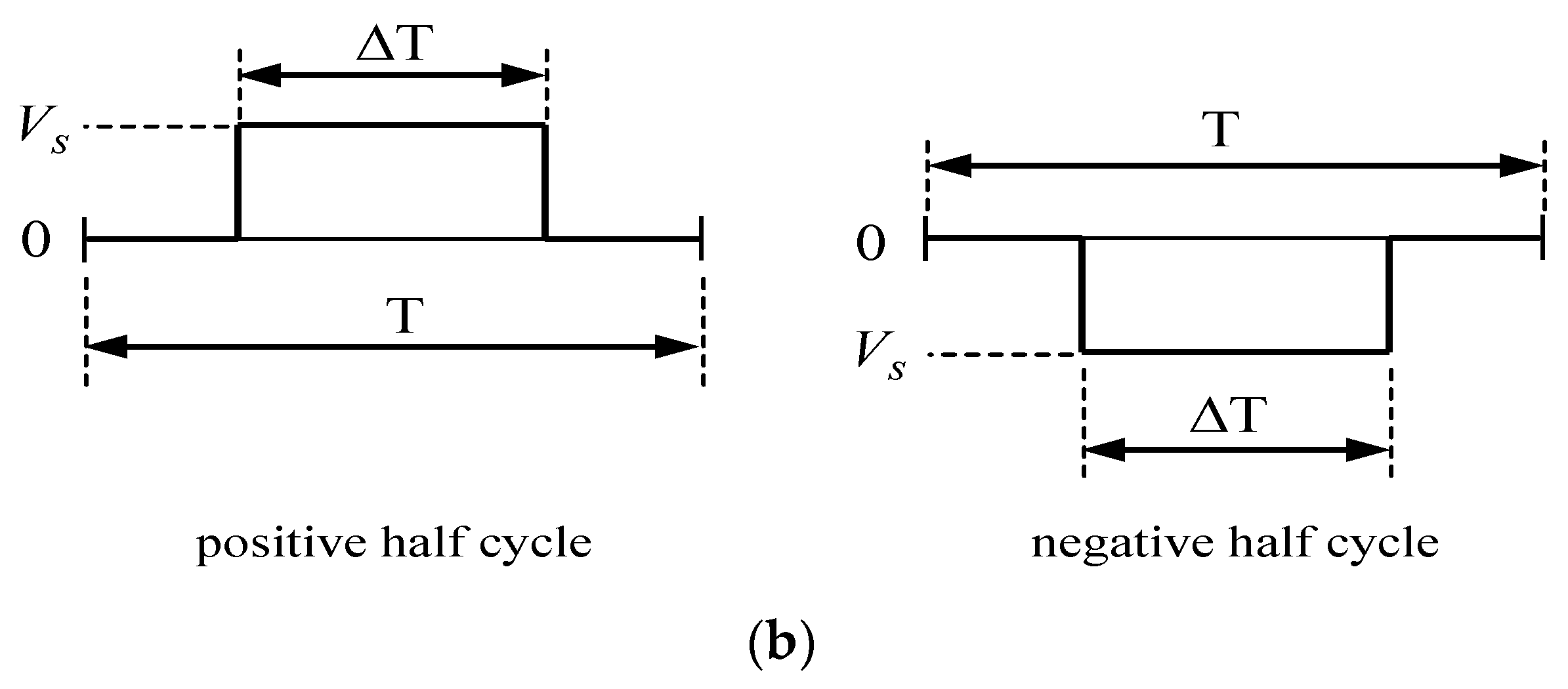
2. Mathematical Representation of VSI

Figure 1a shows a single-phase VSI that is made up of power MOSFET (metal-oxide-semiconductor field-effect transistor), an LC (inductor capacitor) filter and load. The symbol V s represents the DC bus voltage, v o denotes the output voltage, i o is the output current, and L , C , and R are the inductor, capacitor and load, respectively. As shown in Figure 1b, v i n v stands for a pulse width modulated voltage of magnitude V s (or V s ) with Δ T centered in the sampling interval T . Since the inverter output voltage is a sinusoidal waveform, the v o has to follow a desired sinusoidal waveform. For example, for a rms (root mean square) 110 V with a specified frequency of 60 Hz utility power, the v o expected voltage waveform will be 2 110 sin ( 2 π 60 t ) . In other words the output voltage v o of the VSI can be generally expressed as 2 V r m s sin ( 2 π f t ) in which V r m s and f are the root-mean-square and the frequency values of output voltage, respectively. According to the control theory literature [41], we find that the design of the VSI is intrinsically a typical tracking control problem. By choosing x 1 = v o and x 2 = v ˙ o , the dynamic equation of the VSI is derived as:
[ x ˙ 1 x ˙ 2 ] = [ 0 1 1 L C 1 R C ] [ x 1 x 2 ] + [ 0 1 L C ] v i n v  
where a 1 = 1 / L C , a 2 = 1 / R C , b = 1 / L C and v i n v = ( Δ T / T ) V s . The control signal u is equal to d V s (time-averaging technique, see [42,43]), where d is the duty ratio of switching ranging from −1 to 1 and V s denotes the DC bus voltage.
Letting the desired output voltage v d be 2 V r m s sin ( 2 π f t ) , new state variables are defined as:
{ e 1 = x 1 v d   e 2 = x 2 v ˙ d  
By the use of (1) and (2), the error dynamics of a VSI is written as:
[ e ˙ 1 e ˙ 2 ] = [ 0 1 a 1 a 2 ] [ e 1 e 2 ] + [ 0 b ] u + [ 0 Θ ]  
where Θ = a 1 v d a 2 v ˙ d v ¨ d is the uncertainties, such as plant parameter variations, external disturbances and measurement noises. Apparently, we can design u to allow e 1 and e 2 to converge to zero, i.e., x 1 = v d and x 2 = v ˙ d . In the path-tracking control design, it is worth pointing out that once e 1 and e 2 have fast finite time convergence, the system will achieve good performance, strong robustness and infinite stability. Based on the motive for fast finite time convergence and fast convergence property inherited from NFTA, the NFTA VSI will be able to offer not only good dynamic response (fast convergence), but also higher accuracy control (lower THD and tracking error). However, the load of the VSI is not fixed, and the system still has chattering or steady-state error problems when exposed to large step change in loading conditions, extreme parameter variations or highly non-linear loads; the ANFIS can be suggested as an effective way to resolve the chattering or steady-state error in practical applications [44,45,46,47,48,49,50]. Therefore, an intelligent robust tracking controller with the masterly combination of the NFTA and ANFIS compensation for high performance VSI will be presented and the design of the controller is as follows.

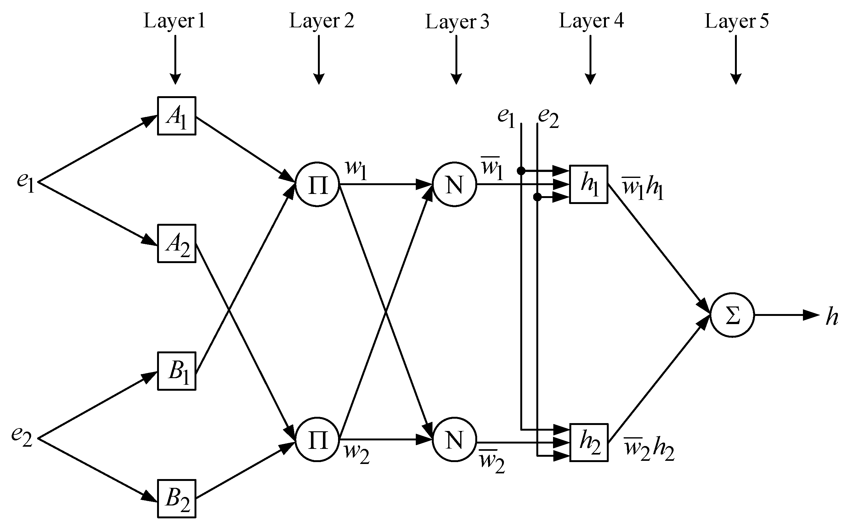
3. Proposed Control Approach of VSI

Problem Statement

Firstly, in this section, the problem statement of the nonlinear system using classic finite-time convergent SMC is presented, and then the proposed controller is designed.
The following second-order nonlinear dynamics are defined as:
{ x ˙ 1 = x 2 x ˙ 2 = f ( x ) + g ( x ) u + Θ ( x )  
where x = [ x 1 x 2 ] T is the state vector, f ( x ) and g ( x ) stand for known nonlinear functions, u represents the control input, and Θ ( x ) symbolizes unknown external disturbances, which are assumed to be bounded as Θ ( x ) < ξ ; here, ξ is positive constant.
A conventional TA can be written as:
σ = x 2 + β | x 1 | γ sgn ( x 1 )  
where β is a positive real number and 0 < γ < 1 . Although TAs can achieve finite-time stability of the system, both the performance and convergence speed of the system are deteriorated while an initial system state stands off the equilibrium. FTA attempts to overcome this problem as follows:
σ = x 2 + α x 1 + β | x 1 | γ sgn ( x 1 )  
where α is a positive real number. When x 1 is far from the zero, the characteristic of the system becomes σ x ˙ 1 + α x 1 , thus yielding exponential stability. When x 1 is close to zero, the FTA is introduced and allows the fast convergence rate of system behavior, which gives rise to finite-time convergence. However, there is still the problem of the singularity appearing in FTA for practical applications.
Eventually for the error dynamics (3), the NFTA can be constructed to ensure faster convergence and precise control without the singularity problem as follows [11,24,25]:
σ = e 1 + α | e 1 | ρ 1 sgn ( e 1 ) + β | e 2 | ρ 2 sgn ( e 2 )  
where α > 0 , β > 0 , ρ 1 > 1 and 1 < ρ 2 > 2 .
The feedback control law of NFTA is designed as:
u ( t ) = u e ( t ) + u s ( t )  
with:
u e ( t ) = b 1 [ a 1 e 1 + a 2 e 2 + 1 β ρ 2 | e 2 | 2 ρ 2 sgn ( e 2 ) + α ρ 1 | e 1 | ρ 1 1 β ρ 2 | e 2 | 2 ρ 2 sgn ( e 2 ) ]  
u s ( t ) = b 1 [ ( ξ + τ ) sgn ( σ ) ]  
where τ > 0 , u e is equivalent control for a nominal system without singular phenomenon, and u s stands for sliding control that arrests external load disturbance. Thereby, the states reach σ = 0 and finite-time convergence is provided.
Proof. 
Choose the following Lyapunov candidate function
V = 0.5 σ 2  
Calculating the derivative of V along the trajectories of (3) gives:
V ˙ = σ σ ˙ = σ ( e ˙ 1 + α ρ 1 | e 1 | ρ 1 1 e ˙ 1 + β ρ 2 | e 2 | ρ 2 1 e ˙ 2 ) = σ β ρ 2 | e 2 | ρ 2 1 [ w ( ξ + τ ) sgn ( σ ) ]
Owing to the existence of σ 0 , e 2 0 and Θ < ξ , V ˙ τ | σ | < 0 , which infers that the σ in (12) can be converged to the equilibrium point within a finite time, a finite system-state convergence time of (3) yields while σ is reached. However, the NFTA may undergo chattering or steady-state error when the load is a severely uncertain circumstance. In order to get rid of the chattering effect, the ANFIS displayed as (13)–(21) is integrated into the control law (8) in the VSI design. Figure 2 plots a common architecture of an ANFIS, which uses the Takagi–Sugeno type fuzzy model with two if-then rules as the following statements [36]:
Rule   1 :   If   e 1   is   A 1   and   e 2   is   B 1   then   h 1 = p 1 e 1 + q 1 e 2 + r 1  
Rule   2 :   If   e 1   is   A 2   and   e 2   is   B 2   then   h 2 = p 2 e 1 + q 2 e 2 + r 2  
where A i and B i symbol the fuzzy sets in the antecedent, and p i , q i and r i signify the design parameters decided in the training duration.
Layer 1: A node function is employed through every node i as:
O i 1 = μ A i ( e 1 ) ,   i = 1 ,   2  
O i 1 = μ B i ( e 2 ) ,   i = 3 ,   4
where μ A i and μ B i can use fuzzy membership functions.
Layer 2: Every node calculating the rule’s firing strength by the multiplier is as follows:
O i 2 = w i = μ A i ( e 1 ) μ B i ( e 2 ) ,   i = 1 ,   2
where w i stands for the output with the firing strength of each rule.
Layer 3: Node i computes the proportion between i th rule’s firing strength and the sum of all rules’ firing strengths. The normalized firing strengths yield:
O i 3 = w ¯ i = w i / ( w 1 + w 2 ) ,   i = 1 ,   2  
Layer 4: Every node i yields the following function:
O i 4 = w ¯ i h i = w ¯ i ( p i e 1 + q i e 2 + r i ) ,   i = 1 ,   2  
where w ¯ i stands for the output of the previous layer, and p i , q i and r i parameters are fuzzy consequent parameters.
Layer 5: The single node of this layer deals with the overall output, summing up to all entered signals as follows:
O i 5 = i = 1 2 w ¯ i h i = ( w 1 h 1 + w 2 h 2 ) / ( w 1 + w 2 )  
The output h shown in Figure 2 can be formulated as:
h = ( w ¯ 1 e 1 ) p 1 + ( w ¯ 1 e 2 ) q 1 + ( w ¯ 1 ) r 1 + ( w ¯ 2 e 1 ) p 2 + ( w ¯ 2 e 2 ) q 2 + ( w ¯ 2 ) r 2  
In summary, the ANFIS architecture is formed by the fuzzy logic model and the artificial neural network, so that the mapping of the inputs to the output is performed. In Figure 2, the basic construction of the ANFIS is illustrated for the first-order Takagi–Sugeno interface system. It is made up of two inputs e 1 and e 2 , and one output h . The first and second layers are regarded as the fuzzification and rule layers, respectively. The first layer deals with the mapping process of the input variable corresponding to each membership functions, and the second layer calculates the rules antecedents. The third layer is called the normalization layer, and the fourth and fifth layers respectively provide the tasks of defuzzification and output. The third layer can normalize the strengths of the rules and then the fourth hidden layer determines the consequents of the rules. Finally, the output layer counts the complete output as the sum of entire arrived signals. In short, the ANFIS permits the choice of the rule base which adapts to the system circumstance. The rule base can be chosen using a backpropagation neural network algorithm. For the sake of increasing the performance, the feature of the fuzzy logic provides the approximation of a nonlinear system via IF-THEN rules that is inherited in this modeling technology. Such a combined method makes ANFIS a universal estimator. □

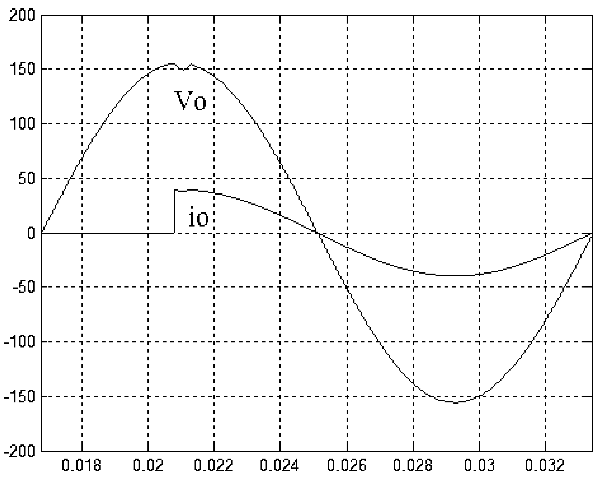
4. Simulation and Experimental Results

The simulation and experimental verification of the presented approach are carried out on a VSI with specifications shown in Table 1. For the sake of the analysis and comparison to the dynamic and steady-state response, the overall system is tested under varying operating conditions, namely step-load changing, filter parameter variations and rectifier loads.
In the simulated waveforms of Figure 3, obtained using the proposed approach, the disturbances caused by the connection of a rated resistive load are presented. After a slight transience, the output voltage quickly recovers to the demanded rms value of 110 V. A good dynamic response and the ability of abrupt disturbance rejection are yielded. Inversely, Figure 4 represents simulated output voltage and output current subject to the same load circumstance obtained using conventional SMC. The large voltage drop and slow recovery time occur while the output voltage has a noticeable oscillation at the back of the transient termination. Figure 5 indicates that the proposed VSI encounters filter parameter variations from 20% to 200% of nominal values with a 12 ohm resistor. The proposed approach is capable of tolerating severe plant parameter variations. Therefore, the simulated output voltage produces a low distorted sinusoidal waveform (%THD is 0.02%). However as expected, the conventional SMC VSI (shown in Figure 6) exhibits low steady-state accuracy with periodic distortion in the simulated output voltage. Namely, it has a high sensitivity to filter parameter variations, resulting in a great deal of voltage harmonics (%THD is 14.32%). Table 2 gives the drop and %THD of the proposed VSI and the conventional SMC VSI in the presence of step load changes and filter parameter variations. A step change in a resistive load (from no load to full load) has been carried out for the experimental waveforms (as shown in Figure 7) obtained using the proposed approach. Under the same load testing condition, Figure 8 depicts the experimental output voltage and output current obtained using the conventional SMC. Comparing of the results from the two figures, the proposed approach yields good compensation for voltage drop mitigation, namely less voltage drop and faster transient recovery time. The output voltage waveform corroborates the robustness of the proposed approach in the presence of load transients. There is no apparent sinusoidal jitter after the occurrence of the transience. Surely, the conventional sliding mode controlled VSI unmasks the performance deterioration—for instance, a large voltage drop when firing at an angle of 90°, slow dynamic response and noticeable vibration behind the transient resumption. To authenticate the performance of the proposed approach under the nonlinear load, Figure 9 plots experimental waveforms in response to a full-wave rectified resistive load (40 Ω) with a DC-side capacitor filter (330 μF). The output voltage of the VSI is close to sine wave and has a low percent THD of 1.82%, which is superior to the five percent industrial standard. Same as the nonlinear load case, the experimental waveforms obtained using the conventional SMC are depicted in Figure 10. The experimental construction is given in Figure 11. The output voltage with a high %THD of 10.21% distorts the resulting waveform, thus leading to large deviation and an unsatisfactory steady-state response. The output voltage drop and %THD of the proposed controlled VSI, as well as the conventional VSI, are listed in Table 3 under step load changes and nonlinear loads. Finally, the improvement of the proposed method really exceeds conventional SMC and is also better than FTA [25].

5. Conclusions

This paper has presented a hybrid controller, which is the association of a robust control technology and machine learning algorithm, to control a voltage source inverter. In this proposed control method, a finite convergence time NFTA offers strong robustness and fast finite-time stability without any singularity. However, if the system is exposed to parametric nonlinearities, parameter variations or unmodelled dynamics, it is not easy to obtain these accurate values completely in practice. As a result, chattering or steady-state error occurs due to the overestimated or underestimated uncertainty bound. The ANFIS with accurate bound estimation is used to tackle and accommodate the uncertain perturbations. The Lyapunov stability criterion displays that the combination of NFTA and ANFIS guarantees the practical finite-time stability of the tracking errors with greater robustness to system uncertainties. Simulations and experiments illustrate that the proposed approach yields very good steady-state and dynamic characteristics under various operating circumstances, such as load step changes, filter parameter variations, and rectifier-type loads.

Author Contributions

E.-C. C. conceived the algorithm, designed the circuit, and performed control system simulations. In addition, E.-C. C. carried out experiments, analyzed the results, wrote the paper and revised it for submission.

Funding

This research was funded by the Ministry of Science and Technology (MOST) of Taiwan, R.O.C., under contract MOST 107-2221-E-214-006.

Acknowledgments

The authors gratefully acknowledge the financial support of the Ministry of Science and Technology of Taiwan, R.O.C., under project number MOST 107-2221-E-214-006.

Conflicts of Interest

The author declares that there is no conflict of interest regarding the publication of this article.

References

  1. Bevrani, H.; Ise, T. Microgrid Dynamics and Control; John Wiley & Sons: Hoboken, NJ, USA, 2017. [Google Scholar]
  2. Sechilariu, M.; Locment, F. Urban DC Microgrid: Intelligent Control and Power Flow Optimization; Elsevier Science Ltd.: Amsterdam, The Netherlands, 2016. [Google Scholar]
  3. Mahmoud, M.S. Microgrid: Advanced Control Methods and Renewable Energy System Integration; Elsevier Science Ltd.: Amsterdam, The Netherlands, 2016. [Google Scholar]
  4. Blaabjerg, F. Control of Power Electronic Converters and Systems; Academic Press: Cambridge, MA, USA, 2018. [Google Scholar]
  5. Sahoo, S.K. Harmonic Analysis of Voltage Source Inverter Using PWM Techniques: Performance Analysis of Three Phase Voltage Source Inverter Using PWM Techniques; LAP LAMBERT Academic Publishing: Riga, Latvia, 2012. [Google Scholar]
  6. Chen, C.; Xiong, R.; Shen, W.X. A Lithium-Ion Battery-in-the-Loop Approach to Test and Validate Multiscale Dual H Infinity Filters for State-of-Charge and Capacity Estimation. IEEE Trans. Power Electron. 2018, 33, 332–342. [Google Scholar] [CrossRef]
  7. He, Y.B.; Chung, S.H.; Ho, N.M.; Wu, W.M. Modified Cascaded Boundary-Deadbeat Control for a Virtually-Grounded Three-Phase Grid-Connected Inverter with LCL Filter. IEEE Trans. Power Electron. 2017, 32, 8163–8180. [Google Scholar] [CrossRef]
  8. Xie, C.A.; Zhao, X.; Savaghebi, M.; Meng, L.; Guerrero, J.M.; Vasquez, J.C. Multirate Fractional-Order Repetitive Control of Shunt Active Power Filter Suitable for Microgrid Applications. IEEE J. Emerg. Sel. Top. Power Electron. 2017, 5, 809–819. [Google Scholar] [CrossRef]
  9. Utkin, V.I. Variable Structure Systems with Sliding Modes. IEEE Trans. Autom. Control 1977, AC-22, 212–222. [Google Scholar] [CrossRef]
  10. Sundarapandian, V.; Lien, C.H. Applications of Sliding Mode Control in Science and Engineering; Springer: Berlin, Germany, 2017. [Google Scholar]
  11. Nabil, D.; Jawhar, G.; Zhu, Q.M. Applications of Sliding Mode Control; Springer: Berlin, Germany, 2017. [Google Scholar]
  12. Bagheri, F.; Komurcugil, H.; Kukrer, O. Fixed switching frequency sliding-mode control methodology for single-phase LCL-filtered quasi-Z-source grid-tied inverters. In Proceedings of the 2018 IEEE 12th International Conference on Compatibility, Power Electronics and Power Engineering (CPE-POWERENG 2018), Doha, Qatar, 10–12 April 2018; pp. 1–6. [Google Scholar]
  13. Abrishamifar, A.; Ahmad, A.; Mohamadian, M. Fixed Switching Frequency Sliding Mode Control for Single-Phase Unipolar Inverter. IEEE Trans. Power Electron. 2012, 27, 2507–2514. [Google Scholar] [CrossRef]
  14. Aamir, M.; Kalwar, K.A.; Mekhilef, S. Proportional-Resonant and Slide Mode Control for Single-Phase UPS Inverter. Electr. Power Compon. Syst. 2017, 45, 11–21. [Google Scholar] [CrossRef]
  15. Hao, X.; Yang, X.; Liu, T.; Huang, L.; Chen, W.J. A Sliding-Mode Controller with Multiresonant Sliding Surface for Single-Phase Grid-Connected VSI with an LCL Filter. IEEE Trans. Power Electron. 2013, 28, 2259–2268. [Google Scholar] [CrossRef]
  16. Khajeh-Shalaly, B.; Shahgholian, G. A Multi-Slope Sliding-Mode Control Approach for Single-Phase Inverters under Different Loads. Electronics 2016, 5, 68. [Google Scholar] [CrossRef]
  17. Lachichi, A.; Pierfederici, S.; Martin, J.P.; Davat, B. Study of a Hybrid Fixed Frequency Current Controller Suitable for DC–DC Applications. IEEE Trans. Power Electron. 2008, 23, 1437–1448. [Google Scholar] [CrossRef]
  18. Zakipour, A.; Shokri-Kojori, S.; Bina, M.T. Closed-loop control of the grid-connected Z-source inverter using hyper-plane MIMO sliding mode. IET Power Electron. 2017, 10, 2229–2241. [Google Scholar] [CrossRef]
  19. Knight, J.; Shirsavar, S.; Holderbaum, W. An improved reliability Cuk based solar inverter with sliding mode control. IEEE Trans. Power Electron. 2006, 21, 1107–1115. [Google Scholar] [CrossRef]
  20. Islam, G.; Muyeen, S.M.; Al-Durra, A.; Hasanien, H.M. RTDS implementation of an improved sliding mode based inverter controller for PV system. ISA Trans. 2016, 62, 50–59. [Google Scholar] [CrossRef] [PubMed]
  21. Montoya, D.G.; Paja, C.A.R.; Giral, R. Improved Design of Sliding-Mode Controllers Based on the Requirements of MPPT Techniques. IEEE Trans. Power Electron. 2016, 31, 235–247. [Google Scholar] [CrossRef]
  22. Yu, X.H.; Wang, B.; Batbayar, B.; Wang, L.P.; Man, Z.H. An improved training algorithm for feedforward neural network learning based on terminal attractors. J. Glob. Optim. 2011, 51, 271–284. [Google Scholar] [CrossRef]
  23. Xiong, J.J.; Zhang, G.B. Global fast dynamic terminal sliding mode control for a quadrotor UAV. ISA Trans. 2017, 66, 233–240. [Google Scholar] [CrossRef] [PubMed]
  24. Mishra, J.; Yu, X.; Jalili, M.; Feng, Y. On fast terminal sliding-mode control design for higher order systems. In Proceedings of the IECON 2016—42nd Annual Conference of the IEEE Industrial Electronics Society, Florence, Italy, 23–26 October 2016; pp. 252–257. [Google Scholar]
  25. Mobayen, S. Fast terminal sliding mode controller design for nonlinear second-order systems with time-varying uncertainties. Complexity 2015, 21, 239–244. [Google Scholar] [CrossRef]
  26. Veluvolu, K.C.; Defoort, M.; Soh, Y.C. High-gain observer with sliding mode for nonlinear state estimation and fault reconstruction. J. Frankl. Inst. 2014, 351, 1995–2014. [Google Scholar] [CrossRef]
  27. Guisser, M.; L-Jouni, A.E.; Abdelmounim, E.L.H. Robust Sliding Mode MPPT Controller Based on High Gain Observer of a Photovoltaic Water Pumping System. Int. Rev. Autom. Control 2014, 7, 225–232. [Google Scholar] [CrossRef]
  28. Vidal-Idiarte, E.; Martinez-Salamero, L.; Gispert, F.G.; Gomariz, S. Sliding and fuzzy control of a boost converter using a 8-bit microcontroller. IEE Proc. Electr. Power Appl. 2004, 151, 5–11. [Google Scholar] [CrossRef]
  29. Cao, J.B.; Cao, B.G. Fuzzy-Logic-Based Sliding-Mode Controller Design for Position-Sensorless Electric Vehicle. IEEE Trans. Power Electron. 2009, 24, 2368–2378. [Google Scholar] [CrossRef]
  30. Radu, S.M.; Tudoroiu, E.R.; Kecs, W.; Ilias, N.; Tudoroiu, N. Real Time Implementation of an Improved Hybrid Fuzzy Sliding Mode Observer Estimator. Adv. Sci. Technol. Eng. Syst. J. 2017, 2, 214–226. [Google Scholar] [CrossRef] [Green Version]
  31. Guzman, R.; Vicuna, L.G.; Morales, J.; Castilla, M.; Miret, J. Model-Based Active Damping Control for Three-Phase Voltage Source Inverters with LCL Filter. IEEE Trans. Power Electron. 2017, 32, 5637–5650. [Google Scholar] [CrossRef] [Green Version]
  32. Fei, J.T.; Zhu, Y.K. Adaptive fuzzy sliding control of single-phase PV grid-connected inverter. In Proceedings of the IEEE Conference on Mechatronics and Automation (ICMA), Changchun, China, 5–8 August 2018; pp. 1233–1238. [Google Scholar]
  33. Wai, R.J.; Lin, Y.F.; Liu, Y.K. Design of Adaptive Fuzzy-Neural-Network Control for a Single-Stage Boost Inverter. IEEE Trans. Power Electron. 2015, 30, 7282–7298. [Google Scholar] [CrossRef]
  34. Mohammad, M. Optimal Operation Management of a Typical Microgrid as Grid Connected in Power Systems Using Fuzzy Sliding-Mode Control (FSMC) Approach. World Appl. Sci. J. 2013, 28, 440–448. [Google Scholar]
  35. Leu, V.Q.; Choi, H.H.; Jung, J.W. Fuzzy Sliding Mode Speed Controller for PM Synchronous Motors with a Load Torque Observer. IEEE Trans. Power Electron. 2012, 27, 1530–1539. [Google Scholar] [CrossRef]
  36. Jang, J.S.R.; Sun, C.T.; Mizutani, E. Neuro-Fuzzy and Soft Computing: A Computational Approach to Learning and Machine Intelligence; Prentice-Hall: Upper Saddle River, NJ, USA, 1997. [Google Scholar]
  37. Vafaei, S.; Rezvani, A.; Gandomkar, M.; Izadbakhsh, M. Enhancement of grid-connected photovoltaic system using ANFIS-GA under different circumstances. Front. Energy 2015, 9, 322–334. [Google Scholar] [CrossRef]
  38. Abdulwahid, A.H.; Wang, S.R. A Novel Approach for Microgrid Protection Based upon Combined ANFIS and Hilbert Space-Based Power Setting. Energies 2016, 9, 1042. [Google Scholar] [CrossRef]
  39. Logeswaran, T.; Senthilkumar, A.; Karuppusamy, P. Adaptive neuro-fuzzy model for grid-connected photovoltaic system. Int. J. Fuzzy Syst. 2016, 17, 585–594. [Google Scholar] [CrossRef]
  40. Garcia, P.; Garcia, C.A.; Fernandez, L.M.; Llorens, F.; Jurado, F. ANFIS-Based Control of a Grid-Connected Hybrid System Integrating Renewable Energies, Hydrogen and Batteries. IEEE Trans. Ind. Inform. 2014, 10, 1107–1117. [Google Scholar] [CrossRef]
  41. Kabzinski, J. Advanced Control of Electrical Drives and Power Electronic Converters; Springer: Berlin, Germany, 2017. [Google Scholar]
  42. Mahdavi, J.; Emaadi, A.; Bellar, M.; Ehsani, M. Analysis of power electronic converters using the generalized state-space averaging approach. IEEE Trans. Circuits Syst. I Fundam. Theory Appl. 1997, 44, 767–770. [Google Scholar] [CrossRef]
  43. Ang, S.; Oliva, A. Power-Switching Converters; CRC Press: Boca Raton, FL, USA, 2010. [Google Scholar]
  44. Noman, A.M.; Addoweesh, K.E.; Alolah, A.I. Simulation and Practical Implementation of ANFIS-Based MPPT Method for PV Applications Using Isolated Ćuk Converter. Int. J. Photoenergy 2017, 2017, 3106734. [Google Scholar] [CrossRef]
  45. Elagori, A.; Tacer, M. Implementation and Evaluation of Maximum Power Point Tracking (MPPT) Based on Adaptive Neuro-Fuzzy Inference System for Photovoltaic PV System. Int. J. Electron. Mech. Mechatron. Eng. 2017, 7, 1453–1474. [Google Scholar]
  46. Shabaan, S.; El-Sebah, I.A.; Bekhit, P. Maximum power point tracking for photovoltaic solar pump based on ANFIS tuning system. J. Electr. Syst. Inf. Technol. 2018, 1, 11–22. [Google Scholar] [CrossRef]
  47. Singh, M.; Chandra, A. Application of Adaptive Network-Based Fuzzy Inference System for Sensorless Control of PMSG-Based Wind Turbine with Nonlinear-Load-Compensation Capabilities. IEEE Trans. Power Electron. 2011, 26, 165–175. [Google Scholar] [CrossRef]
  48. Cheok, A.D.; Wang, Z.F. Fuzzy logic rotor position estimation based switched reluctance motor DSP drive with accuracy enhancement. IEEE Trans. Power Electron. 2005, 4, 908–921. [Google Scholar] [CrossRef]
  49. Senjyu, T.; Kashiwagi, T.; Uezato, K. Position control of ultrasonic motors using MRAC and dead-zone compensation with fuzzy inference. IEEE Trans. Power Electron. 2002, 2, 265–272. [Google Scholar] [CrossRef]
  50. Fotouhi, A.; Auger, D.J.; Propp, K.; Longo, S. Lithium–Sulfur Battery State-of-Charge Observability Analysis and Estimation. IEEE Trans. Power Electron. 2018, 33, 5847–5859. [Google Scholar] [CrossRef]
Figure 1. Construction of voltage source inverter (VSI) (a) Circuit diagram ( V s : DC-bus voltage, v i n v : equivalent output voltage of pulse width modulation, v o : output voltage, i o : output current and R : load); (b) PWM (pulse width modulation) pattern ( T : sampling interval and Δ T : width).
Energies 11 02544 g001aEnergies 11 02544 g001b
Figure 2. Architecture of the adaptive neuro-fuzzy inference system (ANFIS) ( e i : input, A i , B i : linguistic labels, w i : weight and h i : output, for i = 1 ,   2 ).
Energies 11 02544 g002
Figure 3. Simulated output waveforms at step-load changing conditions obtained using the proposed approach (Vo: output voltage; io: output current).
Energies 11 02544 g003
Figure 4. Simulated output waveforms at step-load changing conditions obtained using the conventional sliding mode control (SMC).
Energies 11 02544 g004
Figure 5. Simulation output waveforms against filter parameter variations obtained using the proposed approach.
Energies 11 02544 g005
Figure 6. Simulation output waveforms against filter parameter variations obtained using the conventional SMC.
Energies 11 02544 g006
Figure 7. Experimental output waveforms at step-load changing conditions obtained using the proposed approach (vertical: 100 V/division and 20 A/division, horizontal: 5 ms/division).
Energies 11 02544 g007
Figure 8. Experimental output waveforms at step-load changing conditions obtained using the conventional SMC (vertical: 100 V/division and 20 A/division, horizontal: 5 ms/division).
Energies 11 02544 g008
Figure 9. Experimental output waveforms under rectifier load obtained using the proposed approach (vertical: 100 V/division and 20 A/division, horizontal: 5 ms/division).
Energies 11 02544 g009
Figure 10. Experimental output waveforms under rectifier load obtained using the conventional SMC (vertical: 100 V/division and 20 A/division, horizontal: 5 ms/division).
Energies 11 02544 g010
Figure 11. Experimental construction.
Energies 11 02544 g011
Table 1. VSI system parameters.
Filter Inductor L = 0.1   mH
Filter Capacitor C = 2   μ F
Resistive Load R = 12   Ω
DC link Voltage V s = 200   V
Output Voltage and Frequency v o = 110   V R M S ,   f = 60   Hz
Switching Frequency f s = 12   kHz
Table 2. Simulation comparison of output voltage drop and %THD.
Proposed Approach
Step-load changingFilter parameter variations
Voltage drop%THD
4.6 Vrms0.02%
Conventional SMC
Step-load changingFilter parameter variations
Voltage drop%THD
22.9 Vrms14.32%
Table 3. Experimental comparison of output voltage drop and %THD.
Proposed Approach
Step-load changingRectifier load
Voltage drop%THD
6.5 Vrms1.82%
Conventional SMC
Step-load changingRectifier load
Voltage drop%THD
24.5 Vrms10.21%

