Article

An Improved Ant Lion Optimization Algorithm and Its Application in Hydraulic Turbine Governing System Parameter Identification

1
School of Hydropower and Information Engineering, Huazhong University of Science and Technology, Wuhan 430074, China
2
State Key Laboratory of HVDC Technology (Electric Power Research Institute Co., Ltd., CSG), Guangzhou 510663, China
3
College of Electrical and Electronic Engineering, Huazhong University of Science and Technology, Wuhan 430074, China
*
Author to whom correspondence should be addressed.
Energies 2018, 11(1), 95; https://doi.org/10.3390/en11010095
Submission received: 17 October 2017 / Revised: 27 November 2017 / Accepted: 29 November 2017 / Published: 2 January 2018
(This article belongs to the Section F: Electrical Engineering)

Abstract

:
In this paper, an improved ant lion optimization (IALO) algorithm for parameter identification of hydraulic turbine governing system (HTGS) is proposed. In the proposed algorithm, the search space is explored by the ant lion optimization first, and then the domain is searched by the particle swarm optimization (PSO) in each iteration cycle. A chaotic mutation operation namely Logistics map is introduced for the elite to break out of the local optimum. In mutation operation, a serial-parallel combined method is developed to increase the diversity of mutant population. When the proposed IALO algorithm is applied in the parameter identification of HTGS, the comparative simulation results show that the proposed IALO algorithm has the highest accuracy among different optimization algorithms, and the proposed IALO algorithm has a good convergence characteristic and high stability.

1. Introduction

The accuracy of system parameters is the important foundation of engineering designs and applications. But it is difficult to get accurate parameters from actual prototype directly because of the complexity of hydraulic turbine. Based on the prior knowledge of hydraulic turbine model, the general approach is to estimate the parameters with the identification technology and experiment data [1,2,3]. In the past decades, some existing mature methods, such as least square (LS) [4], genetic algorithm (GA) [5], particle swarm optimization (PSO) [6], bacterial foraging optimization algorithm (BFOA) [7] and Radial Basis Function (RBF) neural network [8], have been applied in parameter identification of hydraulic turbine governing system (HTGS).
Recently, Mirjalili proposed a novel biomimetic optimization algorithm, named ant lion optimization (ALO), by simulating the hunting mechanism of antlions [9]. It has been proved to have good performance in solving optimization problems with advantages of few parameters and high speed. Mirjalili et al., described a multi-objective ALO for solving different multi-objective problems in engineering design [10]. Saxena and Kothari., applied ALO in antenna current and position optimization successfully [11]. Petrović et al., presented effectiveness and applicability of ALO when solving the combinatorial optimization problems for process planning and scheduling [12]. However, like other stochastic algorithms, the phenomenon of prematurity and local optimum may arise for ALO, especially in complex or large scale problems [13].
To eliminate these drawbacks, some new algorithms have been reported. Using a logarithmic fitness function and a ranking selection operator, Gao et al. introduced an improved GA that could estimate the parameters of a hydro generation system model accurately [14]. Liu et al., investigated an enhanced PSO combined with the chaos optimization technique [15]. In [16,17], two different improved gravitational search algorithms (GSA) were developed with different combination strategies of PSO. Liu et al. [18] proposed an improved artificial fish swarm (IAFS) algorithm that was incorporated with the ant colony optimization (ACO) and got good identification results for hydroelectric turbine-conduit.
Inspired by the above literature researches, the following improvements are made in the proposed improved ant lion optimization (IALO) algorithm. Firstly, after searching space by ALO, PSO is introduced to optimize and update the current positions of the antlion group in each iteration. Then, a chaotic mutation operator, namely, Logistics map, is brought into ALO for the elite. It can increase the probability to break out of the local optimum [19]. Finally, a serial-parallel combined method to gain mutant particles is proposed. This can increase the mutation population diversity without additional mutation times. When the proposed ALO algorithm is applied for parameter identification of the HTGS, a six-order state space equation of the HTGS is employed [20,21]. The goal is to get the minimum value of the weighted objective function. The simulation results show that IALO is an effective method with a high accuracy of parameter estimation.
The rest of this paper is as follows. In Section 2, the ALO algorithm and IALO algorithm are introduced, respectively. Section 3 describes the procedures of using IALO algorithm to identify the parameters of HTGS. In Section 4, the simulation results show the effectiveness of IALO. The model and structure of HTGS is shown in Appendix A.

2. The Improved Ant Lion Optimization Algorithm

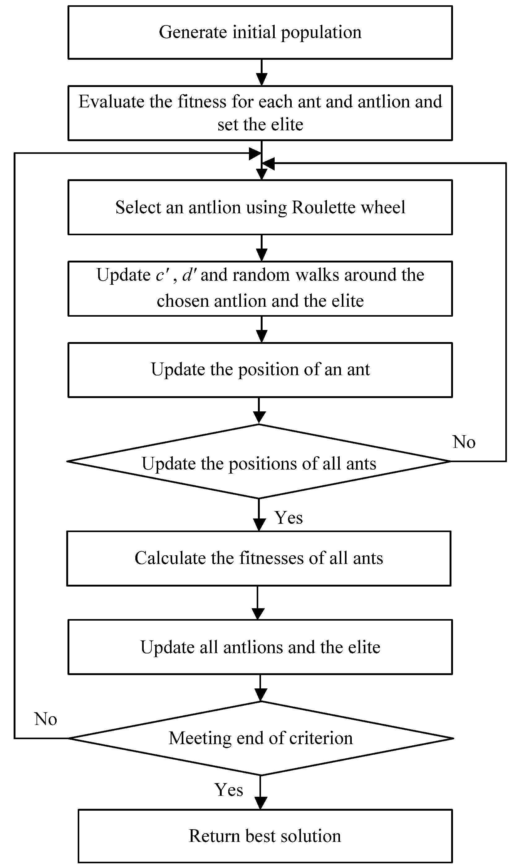
2.1. Brief Introduction of ALO

We briefly sketch the ant lion method here, for a definitive description the reader is referred to [9]. ALO is a new developed stochastic search algorithm, which mimics the hunting mechanism of antlions in nature. In this new approach, ants and antlions as search agents are proposed to find solutions by steps of hunting prey, which includes the random walk of ants, building traps, entrapment of ants in traps, catching prey, and rebuilding traps. The mathematical model of ALO can be described as following.
Ants move stochastically in nature when searching food, therefore a random walk for an ant at each step of optimization process is defined as follows:
X i = [ 0 ;    r ( 1 ) ;       r ( 1 ) + r ( 2 ) ; ;      j = 1 T 1 r ( j ) ;      j = 1 T r ( j ) ]
where i = 1, …, dim, dim is the ant or antlion dimension, T is the maximum number of iteration, X = [X1; …; Xdim], Xi is a (T + 1) × 1 matrix, and r(j) is a stochastic function and can be expressed as:
r = { 1        i f    r a n d > 0.5 1        i f    r a n d 0.5
where rand is a random number generated with uniform distribution in the interval of [0, 1].
Random walks of ants need to be converted to the position in actual search space according to lower and upper boundary. It can be calculated using Equation (3):
Y i = ( X i a i b i a i ) × ( d i c i ) + c i
where ai and bi is the minimum and maximum of Xi, ci, and di indicate the minimum and maximum of antlion in the ith dimension respectively, Y = [Y1; …; Ydim], Yi is a (T + 1) × 1 matrix. Xi is normalized in the domain [0, 1] using X i a i b i a i . Then it is converted into the domain [ci, di] using Equation (3). It means the position around the selected antlion.
The ants’ movements are affected by antlions’ traps. This can be described as:
c = c + A n t l i o n ,          d = d + A n t l i o n
where c’ and d’ is the minimum and maximum of changing limit at current iteration, Antlion is the position of the antlion selected by Roulette wheel, according to the fitnesses.
The possibility of antlions’ building traps is proportional to their fitnesses. Once the antlions know that the ants are trapped and try to escape, the sliding process of ants with decreasing radius occurs. c’ and d’ are updated using Equation (5):
c = l b 10 W × ( t / T ) ,     d = u b 10 W × ( t / T )
where t is the current iteration, lb and ub are the upper limit and lower limit, respectively, W is a constant defined based on the current iteration (W = 2 when t > 0.1 T, W = 3 when t > 0.5 T, W = 4 when t > 0.75 T, W = 5 when t > 0.9 T, W = 6 when t > 0.95 T).
It is easy to find that Y is a (T + 1) × dim matrix calculated in the order of Equations (5), (4), (2), (1), and (3). In the ALO algorithm, Y(t,:) that is based on the MATLAB(R2017a, MathWorks, Natick, MA, USA) format is the final result as the random walk around the chosen antlion.
Besides, elitism is adopted in the ALO algorithm. It means that the best antlion is selected as elite throughout the optimization process. The position update of each ant depends on the random walks around an antlion selected by the Roulette wheel and the elite. It can be determined as:
A n t = R A + R E 2
where Ant is the new position, RA is the random walk around the antlion selected by the Roulette wheel, RE is the random walk around the elite. The new position of the ant should be modified if it is beyond the boundary.
If the ant reaches the bottom of the pit and is fitter than the antlion, then the antlion should take its position. This process is called catching prey and can be given as:
A n t l i o n = A n t , i f    f ( A n t ) < f ( A n t l i o n )
where f(•) is the fitness function.
The flowchart of the ALO algorithm is shown in Figure 1.

2.2. Improvements on ALO

In the ALO algorithm, the ants’ position updates depend on the random walks around the antlion selected by Roulette wheel and the elite, and the best particle is preserved by setting the elite in the searching process. These make ALO have the advantages of fast calculating speed, high efficiency, and good convergence. But, there are phenomenon of the premature convergence and local optimum for complex optimization problems. Some improvements are added to enhance optimization ability and accuracy in this section.

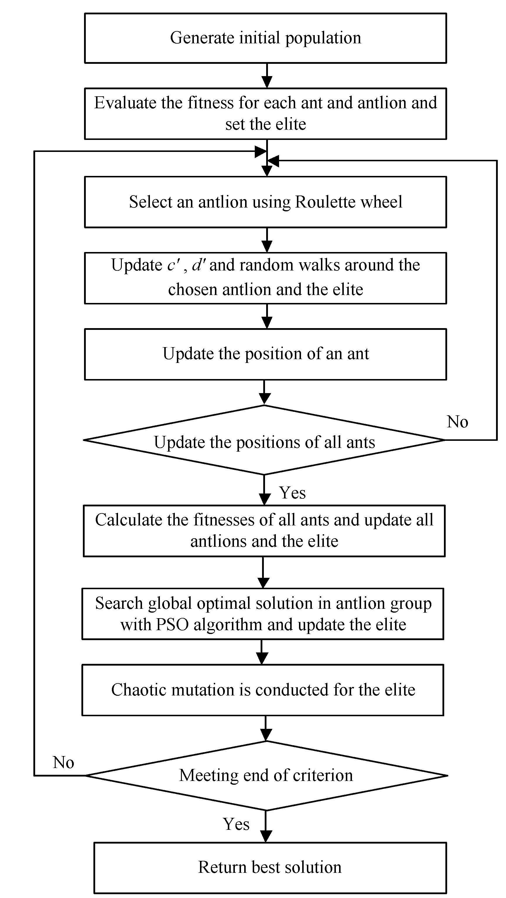
2.2.1. Combination with Particle Swarm Optimization

PSO is a stochastic algorithm that is based on group collaboration by simulating the behavior of birds foraging. As described above, the antlion group is one of crucial parts in the ALO algorithm. So, in this paper, after searching space by ALO, PSO is introduced to optimize and update the current positions of antlions group in each iteration. Through this mechanism, the proposed algorithm has characteristics of both ALO and PSO. The antlions with the ability of communication and memory can move toward the optimal solution faster. In the search strategy of the newly algorithm, the search characteristics of ALO is kept and the communication characteristics of PSO is embedded. This can enhance the search capabilities and improve the searching efficiency in the search period.
The searching strategies of PSO are expressed as [6]:
v i k g + 1 = w v i k g + c 1 r 1 ( p i k g x i k g ) + c 2 r 2 ( B e s t S i k g x i k g )
x i k g + 1 = x i k g + v i k g + 1
where vi is the speed of the ith particle, xi is the position of the ith particle, pi is the best previous position of the ith particle, BestS is the best previous position among all the particles, kg is the current iteration, w is the inertia weight, r1 and r2 are two random variables in the range [0, 1], c1 and c2 are positive constants.

2.2.2. Chaotic Mutation Operator

The mutation operator plays an important role in improving the performance of global searching. It can accelerate the convergence to the optimal solution and maintain the various solutions. In this section, a chaotic mutation operator, namely Logistic map, is incorporated into the improved algorithm and the elite’s position is chosen to be modified by the chaotic mutation. The mathematical function can be written as:
X N + 1 = λ × X N × ( 1 X N )                          0 < λ 4
where N is the current iteration number, λ is a constant.
For different λ, the system of Equation (10) takes on different characteristics. It is not chaotic when 0 < λ < 3. It starts to cycle when λ > 3, and it becomes chaotic status when λ = 4. In this paper, λ is set as 4.

2.2.3. A Serial-Parallel Combined Method to Obtain Mutant Particles

In general, N new particles can be obtained after N mutations of each element in the elite. This commonly used method to get new particles in this case is named parallel method. In this paper, a serial-parallel combined method is proposed. The serial approach is to get the new particles by replacing the corresponding element in the elite with the new mutate element. This new approach ensures stochastic character and increases the diversity of the mutant particles with the same mutation iterations. The procedure is as follows:
(1) Set the elite x0 = (x0(1), …, x0(d), …, x0(dim)), dim is the dimension of the elite, Nm is the iteration number of chaotic mutation.
(2) Loop A: k = 1:Nm
Loop B: d = 1:dim
Convert the position of the elite into a chaos vector y0 in the domain [0, 1]:
y 0 ( d ) = x 0 ( d ) l b ( d ) u b ( d ) l b ( d )
where ub(d) and lb(d) are, respectively, upper limit and lower limit in the dth dimension.
Get a new element by Logistic map as follows:
y k ( d ) = 4 × y k 1 ( d ) × ( 1 y k 1 ( d ) )
where k is the kth iteration, λ is set as 4.
Convert yk(d) into the actual position as follows:
x k ( d ) = l b ( d ) + y k ( d ) × ( u b ( d ) l b ( d ) )
Replace x0(d) with xk(d). Obtain the new particle xnew = (x0(1), …, xk(d), …, x0(dim)) and calculate its fitness. If xnew is better, replace x0 with xnew.
End Loop B.
Obtain the new particle xk = (xk(1), …, xk(d), …, xk(dim)) and calculate the fitness. If xk is better, replace x0 with xk.
End Loop A.
Through chaotic mutation and the series-parallel combined method to obtain mutant particles, there is greater possibility to make the elite to overstep the local optimum and get a better solution for the new algorithm.
According to the above improvements to the ant lion optimization (ALO), IALO is summarized below. Figure 2 shows the flowchart of the newly IALO algorithm. In the following sections, IALO will be applied to identify the parameters of HTGS and the identification experiments will be used to demonstrate the validity and feasibility of IALO.
The steps of the IALO algorithm are described as follows:
Step 1: Initialization. Randomly initialize the positions of ants and antlions.
Step 2: Calculate the finesses of the antlions and choose the antlion whose fitness is best as the elite.
Step 3: Select an antlion using Roulette wheel and calculate the random walks around the chosen antlion and the elite. Update the ants’ position with Equations (5), (4), (2), (1), (3), and (6).
Step 4: Repeat Step 3 until the positions of all the ants are updated.
Step 5: Update the antlions’ positions with Equation (7). Compare fitnesses of the new antlions with the fitness of the elite. If the antlion has better fitness than the elite, then the elite will be replaced by the position of the antlion.
Step 6: PSO is adopted to search better antlions with Equations (8) and (9). Update the elite.
Step 7: Chaotic mutation is conducted for the elite and gets the mutant particles using a serial-parallel combined method with Equations (11)–(13).
Step 8: Repeat Step 3 to Step 7 until the stop criteria are met.

3. Parameter Identification for HTGS Based on IALO

In general, an unknown parameters identification problem with known model structure and selected algorithm can be turned into an optimization problem. After exciting the original system, a defined objective function should be expressed with the original system outputs and identified system outputs. Then, the unknown parameters vector can be taken as a particle and the objective function will be minimized in the optimization process. When the responses of original system and identified system are in better agreement, the estimated parameters are closer to the true values.

3.1. Objective Function

The detailed model of HTGS is introduced in Appendix A. In this section, turbine speed x, guide vane opening y, and turbine torque mt are selected as output variables. In the HTGS, kp, ki, and kd can be directly read from the PID controller and Ty can be measured in the special experiment for the servo-mechanism. Therefore, we choose θ = [Tw Te f Taeg] as the identified parameter vector. In Ref. [16], a new objective function with weights that represent the importance of each parameter is proposed and the weights are calculated with the outputs deviation. This new objective is a weighted least squares error between the actual and estimated output vectors. It can be defined as:
C I O F ( θ ) = k = 1 L j = 1 n w j ( z j ( k ) z ^ j ( k ) ) 2
where z = [x y mt] is the output vector of real system, z ^ = [ x ^        y ^        m t ^ ] is the output vector of estimated model, L is the number of samples, n is the dimension of system output vector, n = 3. The output vector is measured at a number of different times when calculating the weights in the objective. The weight vector w = [w1 w2 w3] is calculated according to following steps:
(1) Set value of each vector parameter θi, i = 1, …, m(m is the dimension of parameter vector θ, m = 5), and get system output vector z = [z1(k), …, zn(k)], k = 1, …, L.
(2) Loop: i = 1:m
Change the ith parameter’s value, θ n e w = θ i × ( 1 + Δ % ) , and obtain system output vector z ^ i = [ z ^ i 1 ( k ) , ... , z ^ i n ( k ) ] .
End Loop.
(3) Calculate g j = i = 1 m k = 1 L ( z j ( k ) z ^ i j ( k ) ) 2 , j = 1, …, n.
(4) Calculate the jth weight w j = g j j = 1 n g j .

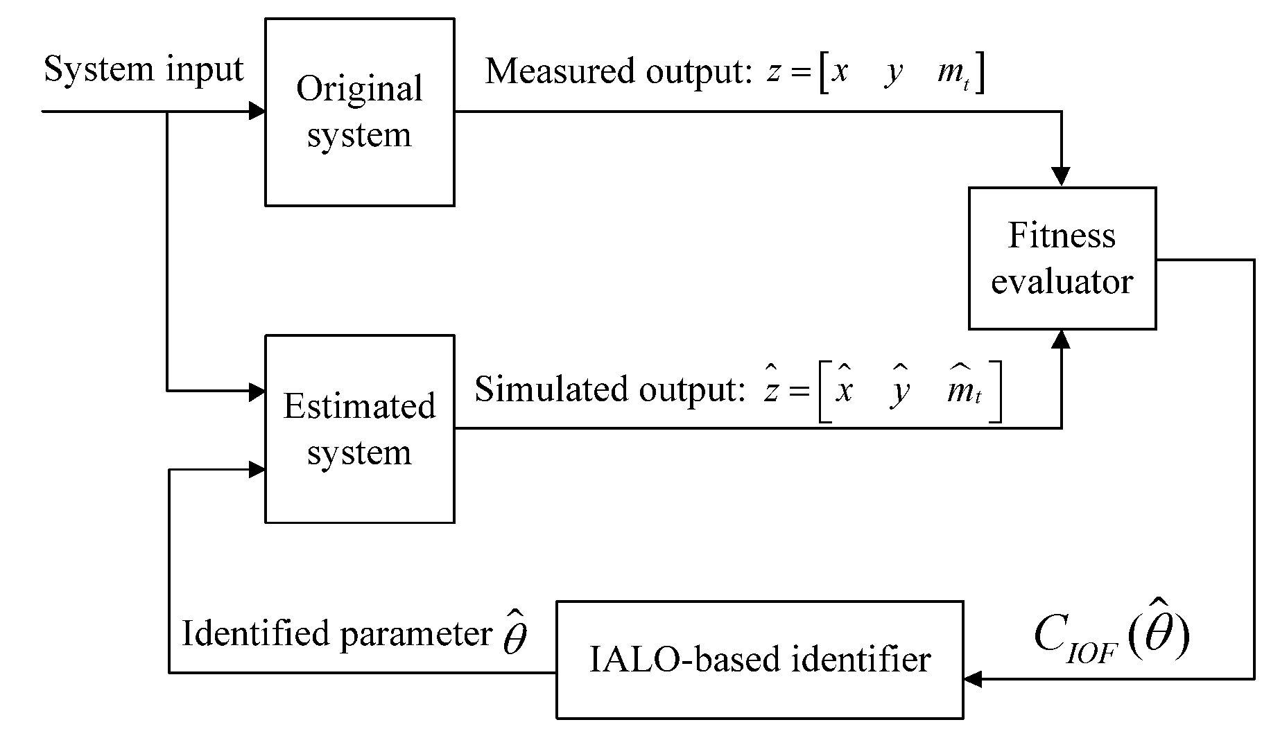
3.2. Parameter Identification Strategy

Figure 3 is the diagram of IALO based HTGS parameter identification. At first, a suitable input signal is chosen to excite both the original system and the estimated system. The obtained measured output and simulated output as inputs in the fitness evaluator are used to calculate the fitness. Then, in IALO-based identifier, the unknown parameter vector θ ^ is identified by minimizing the fitness function CIOF( θ ^ ). So, this cycle continues, the identified parameters approximate to the real values gradually.
Parameter identification accuracy is measured by parameter error (PE):
P E = | θ i θ ^ i θ i | × 100 % , i = 1 , 2 , , m
and average parameter error (APE):
A P E = 1 m i = 1 m | θ i θ ^ i θ i | × 100 %
where θi is the parameter in original system, θ ^ i is the parameter in estimated system, m is the dimension of θ.

4. Experiments and Results Analysis

In this part, the HTGS is simulated in MATLAB, and the proposed IALO is applied to identify five key parameters of simulated system, which are Tw, Te, f, Ta, and eg. The structure and model of HTGS are respectively described in Appendix A Figure A1 and Figure A2.
For high reliability of results, two experiments, which are under no-load and load operations, are considered for the parameter identification of HTGS, and step disturbances of given speed and load are, respectively, adopted to excite system. When considering the engineering practice, the amplitudes of step disturbance of speed and load are set as 0.04 p.u. and 0.1 p.u., respectively. The parameters of simulation models of HTGS are set as follows:
For PID controller, the proportional gain kp = 5.5912, the integral gain ki = 1.0611, the differential gain kd = 3.2800, the differential time constant T1v = 0.28, the feedback coefficient bp = 0.04. For servomechanism, the inertia time constant Ty = 0.1. For the hydraulic system, the water time constant Tw = 1.5, the water travel time Te = 0.53, the friction losses f = 0.01. The transfer coefficients of turbine under different conditions are shown in Table 1. For the generator and load, the inertia time constant of generator and load Ta’ = 12, the adjusting parameter of generator eg = 0.4433.
In the simulation experiments, the true value of the identified parameter vector in the original system is θ = [1.5 0.53 0.01 12 0.4433], the upper limit and lower limit are respectively set as ub = [2 1 0.05 20 1] and lb = [0 0 0 0 0]. The simulation time is 30 s and the sampling time is 0.01 s. They are enough to ensure that the system becomes stable from transient process and the details of dynamic process can be captured.

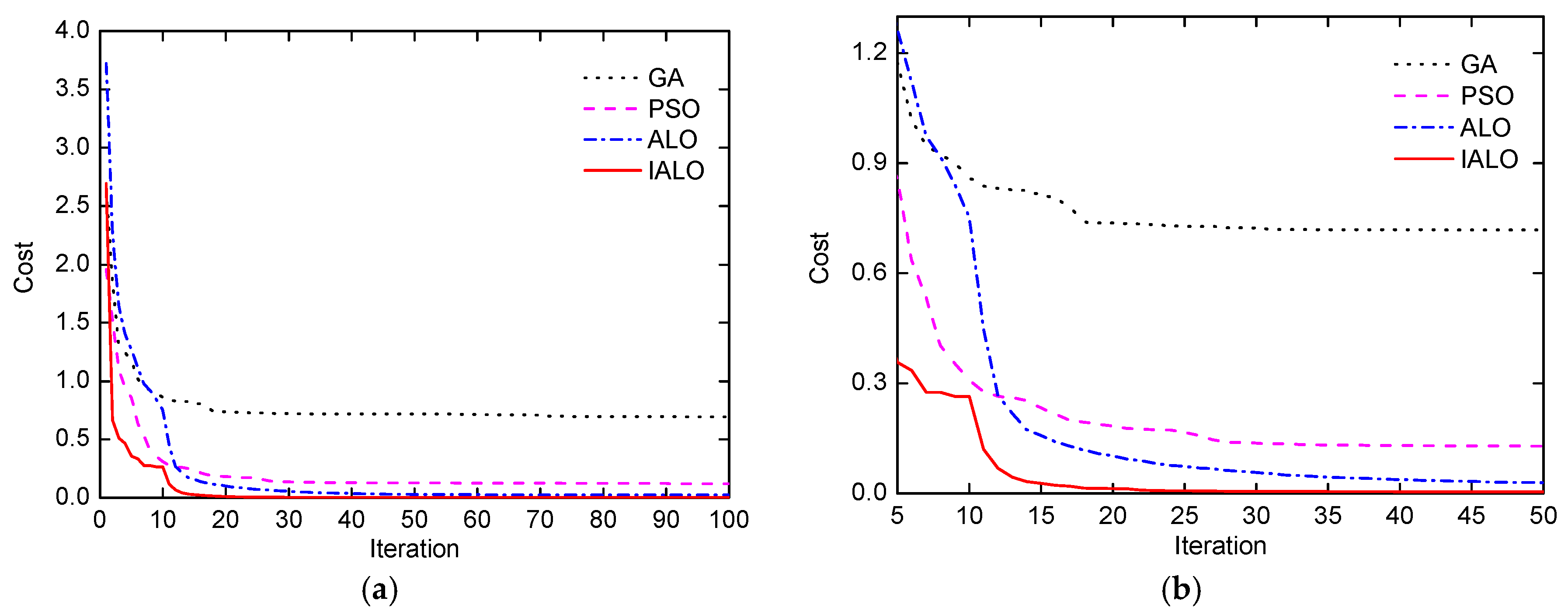
4.1. Comparison of Different Identification Methods under No-Load Condition

In this section, the system is under no-load condition and GA, PSO, ALO, and IALO are used to identify the parameters of HTGS. In the identification process, to compare fairly well the performance of different algorithms, population size and iteration number of GA, PSO, ALO, and IALO are all set as 30 and 100, respectively. For GA, crossover rate Pc = 0.7, mutational rate Pm = 0.06. For PSO, w = 0.6, c1 = c2 = 2. For IALO, w = 0.6, c1 = c2 = 2, Np = 1(Np is the iteration number of PSO), Nm = 5. In order to reduce the random error, the simulation experiments are repeated 20 times and the final results are the average value for each algorithm.
Table 2 shows the value and PE of the identified parameters for different algorithms. Mean best cost and mean APE are listed in Table 3. From Table 2 and Table 3, it is easy to find that IALO is the best for three accuracy indexes. It means that the parameters that are estimated by IALO are closer to the real values than ones estimated by GA, PSO and ALO.
The average iteration processes and the local magnification of different methods under no-load operation are compared in Figure 4. It is shown that GA gets local optimal solution early. PSO achieves better results than ALO at the beginning of the iteration process, but the prematurity phenomenon appears at middle and late stage. IALO could achieve faster convergence to the optimal and get better global optimum solution than the others.
Figure 5 shows the comparisons of the original system outputs and the estimated system outputs, which are obtained with the parameters identified by IALO. The output variables in comparisons are guide vane opening, turbine torque and turbine speed. It is obvious that the estimated curves agree well with original curves. It indicates that IALO is sufficiently effective for the parameter identification of HTGS.

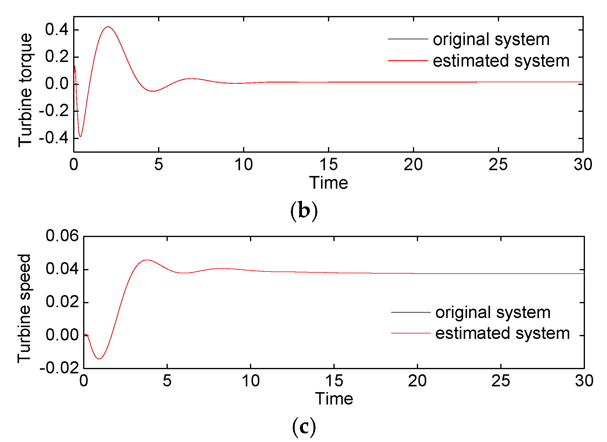
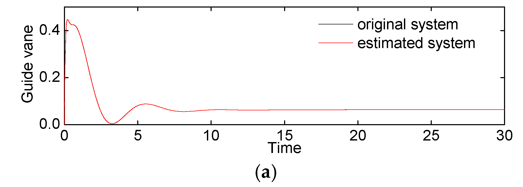
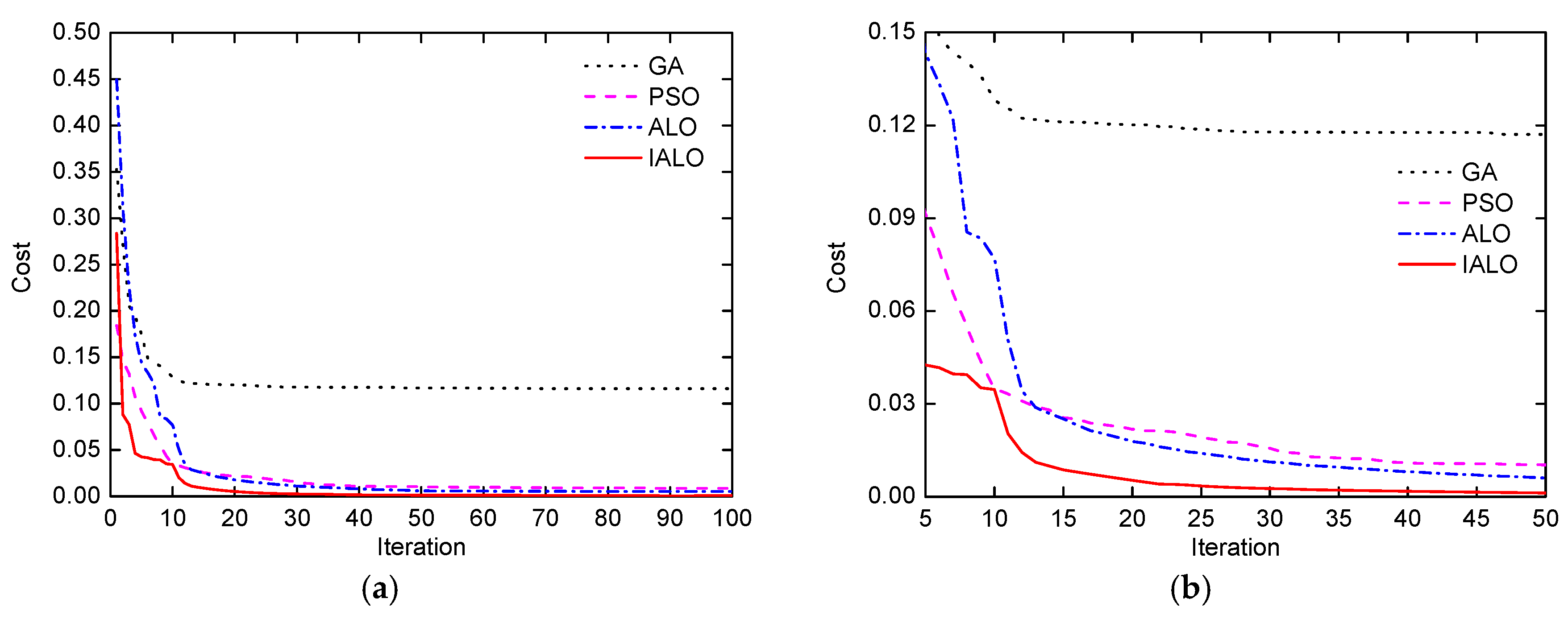
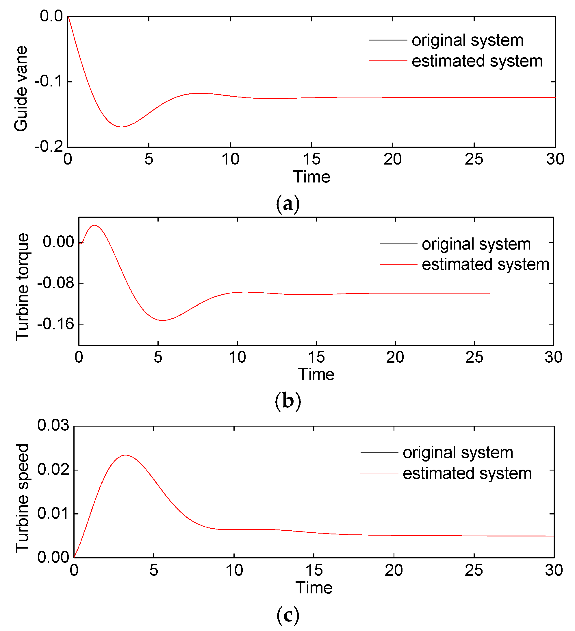
4.2. Comparison of Different Identification Methods under Load Condition

In this part of experiments, the system is under load condition, and GA, PSO, ALO, and IALO are applied to the parameters identification of HTGS. The parameters of GA, PSO, ALO, and IALO are not changed. Similarly, the tests are repeated 20 times and the average of all the tests is calculated.
The values and PE of identified parameters for different methods are listed in Table 4. Table 5 shows the mean best cost and mean APE of each algorithm. From Table 4 and Table 5, it can be observed that IALO has higher accuracy of parameter identification compared to GA, PSO, and ALO. The mean best cost and mean APE that are obtained by IALO are as small as 0.0010 and 0.0808, respectively.
The comparison of average convergence curves and local magnification of different algorithms are illustrated in Figure 6. It is clear that IALO has a better ability to jump from local optimal solution than GA, PSO, and ALO. The estimated output curves using IALO and original output curves under load condition are compared in Figure 7. It is seen that the estimated curves agree well with the original curves. It means that the identified system using the parameters by IALO is very close to the original system.

5. Conclusions

In this paper, an IALO algorithm is developed to identify the parameters of HTGS. The proposed IALO has better search ability with combination of search strategy of PSO. Logistics map as mutation operator is adopted to enhance ability of escaping from local optimal solution. The proposed serial-parallel combined method can increase the diversity of mutation population. The simulation experiment results show that IALO has high accuracy and good stability. Meanwhile, a model of HTGS with a reduced order water hammer equation and engineering experience is built, and the amplitudes of excitation signals are set based on engineering application.

Acknowledgments

This paper is supported by the National Natural Science Foundation of China (No. 51479077), the Fundamental Research Funds for the Central Universities of China (No. 2017KFYXJJ208) and the Science and Technology Program of CSG (No. K-KY2014-007).

Author Contributions

All authors contributed in developing the idea of this research. Changyu Liu, Qi Guo, Yi Yuan, Wei Li and Qiurong Yan conceived the study; Tian Tian proposed the algorithm. All authors discussed the drafts.

Conflicts of Interest

The authors declare no conflict of interest.

Appendix A

HGTS is a complicated closed-loop system, mainly includes three parts, i.e., hydraulic turbine governor, hydraulic system, generator and load. Figure A1 shows the structure of HTGS. Each subsystem is introduced respectively.
Figure A1. Structure of hydraulic turbine governing system.
Energies 11 00095 g0a1

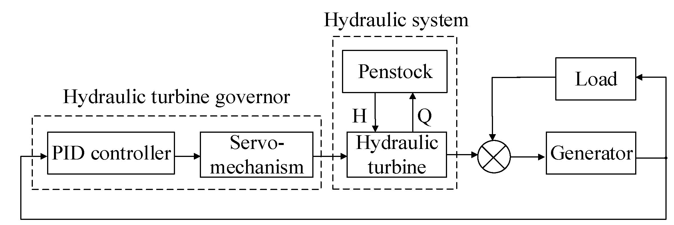
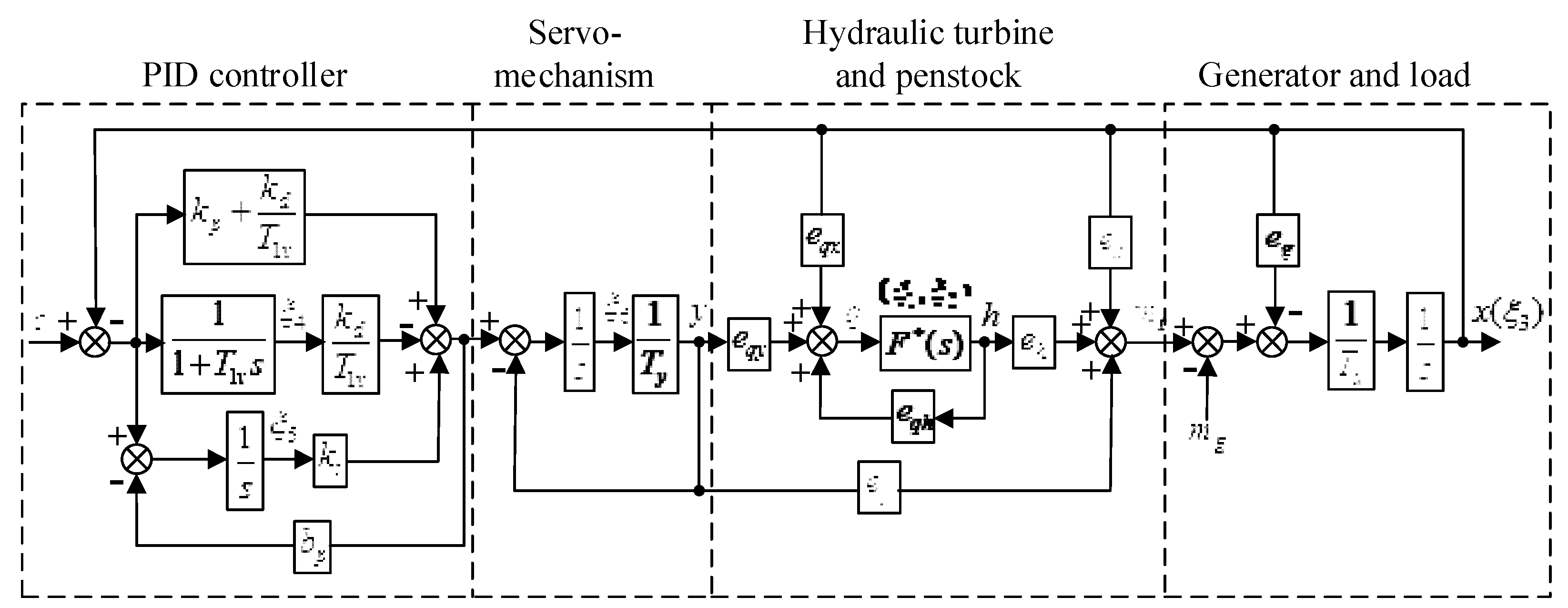
(1) Model of Hydraulic Turbine Governor

Hydraulic turbine governor consists of controller and servomechanism. In general, the parallel PID control law is widely used. The PID controller could be expressed as:
σ ( s ) c ( s ) x ( s ) = 1 1 + b p k i s ( k p + k i s + k d s 1 + T 1 v s )
where s is the Laplace operator, c is the given speed, x is the generator unit speed, σ is the output of PID controller, kp, ki and kd are the proportional gain, integral gain and differential gain, T1v is differential time constant, bp is feedback coefficient. All variables are relative deviations.
The servomechanism is the actuator of governor, which is used to operate the guide vane of hydraulic turbine according to the output signal of PID controller. The transfer function of servomechanism could be shown as:
y ( s ) σ ( s ) = 1 T y s + 1
where y is the guide vane opening, Ty is the inertia time constant of servomechanism.

(2) Model of Hydraulic System

In the HTGS, hydraulic system is the one of important subsystems which provides prime mover and mainly contains hydraulic turbine, penstock and surge tank. The process of water flow in a turbine is complicated. In principle, the dynamic characteristics of hydraulic turbines should be used in the analysis of hydraulic turbine governing systems, but it is impossible to get the characteristics by model tests actually. The engineering practice has proved that when the system is in steady operation and the turbine speed varies in a small range, the theoretical results obtained from the steady state characteristics of hydraulic turbine are in good agreement with the measured results [20].
In actually, the mathematical model of hydraulic system can be considered into three parts:
(1) Hydraulic turbine converts water power into mechanical energy and drives the generator to generate electricity. In a neighborhood of an operating point, the turbine torque mt and the flow q can be expressed with linear functions of guide vane opening y, water head h and speed x. Steady state characteristics of hydraulic turbine could be shown as:
m t ( s ) = e x x ( s ) + e y y ( s ) + e h h ( s )
q ( s ) = e q x x ( s ) + e q y y ( s ) + e q h h ( s )
where ex, ey, eh, eqx, eqy and eqh are transfer coefficients of hydraulic turbine.
(2) The fluid characteristics of penstock can be taken as part of flow inertia of pressure discharge system. In the penstock, the sudden changes in flow will cause severe changes in water head. We call that the water hammer. The dynamic process can be described as:
F ( s ) = h ( s ) q ( s ) = T w T e tanh ( T e s + f )
where Tw is the water time constant, Te is the water travel time, f is the friction losses in the penstock.
The water hammer transfer function is a hyperbolic tangent function, which will lead to algebraic loop problem in the simulation. The general approach to solve this problem is to approximate it with a reduced-order model using Taylor series. The first-order (inelastic) or third-order (elastic) water hammer equation are adopted traditionally in most studies, but there are still shortcomings of accuracy in the frequency domain. A reduced order water hammer equation with advantages of good approximation accuracy and low order is introduced in Ref. [21]. The equation could be shown as:
F ( s ) = T w T e 2 f T e 2 π 2 s 2 + T e s + f s 2 + 4 f T e π 4 + 2 f 2 s + 1
(3) The mechanical inertia of the flow in the rotor and runner of hydraulic turbine can be accounted as a part of hydro-generator unit’s mechanical inertia.

(3) Model of Generator and Load

In the study of HTGS, the generator and load system is often simplified as a one-order system. The electromagnetic effects are usually ignored and the inertia of the synchronous generator is only considered. The transfer function could be expressed as:
x ( s ) m t ( s ) m g ( s ) = 1 T a s + ( e g e x )
where mg is the load torque, Ta’ = Ta + Tb, Ta is the inertia time constant of generator, Tb is inertia time constant of load, eg is the adjusting coefficient of generator.
Figure A2 is the mathematical model of HTGS. In order to describe the multiple-input and multiple-output system better, a six-order state space equation is adopted in this paper. For convenience of selecting the state variables, the following changes are made to the PID controller: k d s 1 + T 1 v s = k d T 1 v k d / T 1 v T 1 v s + 1 . ξ = [ ξ 1      ξ 2      ξ 3      ξ 4      ξ 5      ξ 6 ] T ( ξ 1 and ξ 2 are the state variables in the transfer function F ( s ) ) is the state vector, and u = [mg c]T and z = [x y mt]T are selected as input vector and output vector respectively. The corresponding state equation for HTGS could be written as:
Figure A2. Block diagram of transfer functions of HTGS.
Energies 11 00095 g0a2
ξ = [ 0 a 12 0 0 0 0 a 21 a 22 a 23 0 0 a 26 a 31 a 32 a 33 0 0 a 36 0 0 a 43 a 44 0 0 0 0 a 53 a 54 a 55 0 0 0 a 63 a 64 a 65 a 66 ] ξ · + [ 0 0 0 0 b 31 0 0 b 42 0 b 52 0 b 62 ] u
z = [ 0 0 c 13 0 0 0 0 0 0 0 0 c 26 c 31 c 32 c 33 0 0 c 36 ] ξ
where a 12 = 1 , a 21 = π 2 4 T e 2 + π 2 e q h f T w 8 T e 2 + 4 e q h T w f T e 2 , a 22 = π f T e 4 + 2 f 2 + e q h π 2 T w + 2 π T w f 2 / ( T e 4 + 2 f 2 ) 4 T e + 2 T w f e q h , a 23 = e q x 2 T e T w f e q h e q x 2 T e + e q h T w f , a 26 = e q y T y e q y e q h T w f T y ( 2 T e + e q h T w f ) , a 31 = π 2 f T w e h 4 T a T e 2 ( T e + e q h f T w ) , a 32 = π 2 T w e h + 2 π T w f 2 e h / ( T e 4 + 2 f 2 ) 2 T a ( 2 T e + T w f e q h ) , a 33 = 1 T a ( e x e g 2 T e T w f e q x e h 2 T e + e q h T w f ) , a 36 = 1 T a T y ( e y 2 T e T w f e q h e h 2 T e + e q h T w f ) , a 43 = 1 T 1 v , a 44 = 1 T 1 v , a 53 = b p ( k p + k d T 1 v ) 1 , a 54 = b p k d T 1 v , a 55 = b p k i , a 63 = k p k d T 1 v , a 64 = k d T 1 v , a 65 = k i , a 66 = 1 T y , b 31 = 1 T a , b 42 = 1 T 1 v , b 52 = 1 b p ( k p + k d T 1 v ) , b 62 = k p + k d T 1 v , c 13 = 1 , c 26 = 1 T y , c 31 = π 2 f T w e h 8 T e 2 + 4 e q h T w f T e 2 , c 32 = π 2 T w e h + 2 π T w f 2 e h / ( T e 4 + 2 f 2 ) 4 T e + 2 T w f e q h , c 33 = e x 2 T e T w f e q x e h 2 T e + e q h T w f , c 36 = e y T y 2 T e T w f e q h e h T y ( 2 T e + e q h T w f ) .

References

  1. Demello, F.P.; Koessler, R.J.; Agee, J.; Anderson, P.M.; Doudna, J.H.; Fish, J.H.; Hamm, P.A.L.; Kundur, P.; Lee, D.C.; Rogers, G.J.; et al. Hydraulic turbine and turbine control models for system dynamic studies. IEEE Trans. Power Syst. 1992, 7, 167–179. [Google Scholar] [CrossRef]
  2. De Jaeger, E.; Janssens, N.; Malfliet, B.; Van De Meulebroeke, F. Hydro turbine model for system dynamic studies. IEEE Trans. Power Syst. 1994, 9, 1709–1715. [Google Scholar] [CrossRef]
  3. Trudnowski, D.J.; Agree, J.C. Identifying a hydraulic-turbine model from measured field data. IEEE Trans. Energy Convers. 1995, 10, 763–768. [Google Scholar] [CrossRef]
  4. Liu, C.Y.; Liang, X.L. Model identification of controlled subject for hydro turbine governing system. Water Resour. Power 2007, 25, 77–79. [Google Scholar] [CrossRef]
  5. Yang, X.D.; Dong, C.; Lu, W.H. Parameters identification for hydraulic turbine governing systems based on genetic algorithm. Relay 2006, 34, 27–30. [Google Scholar] [CrossRef]
  6. Liu, C.; Liu, N.; Sun, X.; Cui, J. The research and application on parameter identification of hydraulic turbine regulating system based on particle swarm optimization and uniform design. In Proceedings of the International Conference on Computer Science and Information Technology (ICCSIT 2010), Chengdu, China, 9–11 July 2010; pp. 605–608. [Google Scholar]
  7. Kuo, P.; Zhou, J.; Li, C.; He, H. Identification of hydraulic turbine governor system parameters based on bacterial foraging optimization algorithm. In Proceedings of the Sixth International Conference on Natural Computation (ICNC 2010), Yantai, China, 10–12 August 2010; pp. 3339–3343. [Google Scholar]
  8. Xiao, Z.; Wang, S.; Zeng, H.; Yuan, X. Identifying of hydraulic turbine generating unit model based on neural network. In Proceedings of the IEEE International Intelligent System Design and Applications, Jinan, China, 16–18 October 2006; pp. 113–117. [Google Scholar] [CrossRef]
  9. Mirjalili, S. The ant lion optimizer. Adv. Eng. Softw. 2015, 83, 80–98. [Google Scholar] [CrossRef]
  10. Mirjalili, S.; Jangir, P.; Saremi, S. Multi-objective ant lion optimizer: A multi-objective optimization algorithm for solving engineering problems. Appl. Intell. 2016, 1–17. [Google Scholar] [CrossRef]
  11. Saxena, P.; Kothari, A. Ant lion optimization algorithm to control side lobe level and null depths in linear antenna arrays. AEU Int. J. Electron. Commun. 2016, 70, 1339–1349. [Google Scholar] [CrossRef]
  12. Petrović, M.; Petronijević, J.; Mitić, M.; Vuković, N.; Miljković, Z.; Babić, B. The ant lion optimization algorithm for integrated process planning and scheduling. Appl. Mech. Mater. 2016, 834, 187–192. [Google Scholar] [CrossRef]
  13. Man, K.F.; Tang, K.S.; Kwong, S. Genetic algorithms: Concepts and applications. IEEE Trans. Ind. Electron. 1996, 43, 519–534. [Google Scholar] [CrossRef]
  14. Gao, L.; Dai, Y.; Xia, J. Parameter identification of hydro generation system with fluid transients based on improved genetic algorithm. In Proceedings of the Fifth International Conference on Natural Computation (ICNC 2009), Tianjin, China, 14–16 August 2009; pp. 398–402. [Google Scholar]
  15. Liu, B.; Wang, L.; Jin, Y.; Tang, F.; Huang, D. Improved particle swarm optimization combined with chaos. Chaos Solitons Fractals 2005, 25, 1261–1271. [Google Scholar] [CrossRef]
  16. Li, C.; Zhou, J. Parameters identification of hydraulic turbine governing system using improved gravitational search algorithm. Energy Convers. Manag. 2011, 52, 374–381. [Google Scholar] [CrossRef]
  17. Chen, Z.; Yuan, X.; Tian, H.; Ji, B. Improved gravitational search algorithm for parameter identification of water turbine regulation system. Energy Convers. Manag. 2014, 78, 306–315. [Google Scholar] [CrossRef]
  18. Liu, C.Y.; He, X.S.; Li, C.W.; Wang, Z.; Zhang, E.B. Improved artificial fish swarm algorithm for parameter identification of hydroelectric turbine-conduit system. Electr. Power Autom. Equip. 2013, 33, 54–58. [Google Scholar] [CrossRef]
  19. Lampart, M.; Oprocha, P. Chaotic sub-dynamics in coupled logistic maps. Phys. D Nonlinear Phenom. 2016, 335, 45–53. [Google Scholar] [CrossRef]
  20. Shen, Z.Y. Hydraulic Turbine Regulation, 3rd ed.; Water Power Press: Beijing, China, 1988; pp. 181–199. ISBN 9787801244123. [Google Scholar]
  21. Liu, C.Y.; He, X.S.; He, F.J.; Wang, G.H.; Lin, Y.; Yan, Q.R. Refined modeling of hydraulic prime mover and its governing system for hydropower generation unit. Power Syst. Technol. 2015, 39, 230–235. [Google Scholar] [CrossRef]
Figure 1. Flowchart of the ant lion optimization (ALO) algorithm.
Energies 11 00095 g001
Figure 2. Flowchart of the improved ant lion optimization (IALO) algorithm.
Energies 11 00095 g002
Figure 3. Diagram of IALO based hydraulic turbine governing system (HTGS) parameter identification.
Energies 11 00095 g003
Figure 4. (a) Comparison of average iteration process under no-load condition; (b) Local magnification of average iteration process under no-load condition.
Energies 11 00095 g004
Figure 5. Comparison of system outputs using IALO under no-load condition. (a) Guide vane curves of the original system and the estimated system; (b) Turbine torque curves of the original system and the estimated system; (c) Turbine speed curves of the original system and the estimated system.
Energies 11 00095 g005aEnergies 11 00095 g005b
Figure 6. (a) Comparison of average iteration process under load condition; (b) Local magnification of average iteration process under load condition.
Energies 11 00095 g006
Figure 7. Comparison of system outputs using IALO under load condition. (a) Guide vane curves of the original system and the estimated system; (b) Turbine torque curves of the original system and the estimated system; (c) Turbine speed curves of the original system and the estimated system.
Energies 11 00095 g007
Table 1. Transfer coefficients of hydraulic turbine under two conditions.
Working ConditionTransfer Coefficients of Turbine
exeyeheqxeqyeqh
No-load−1.05670.90801.4191−0.05740.78870.4571
Load−1.46730.77131.7179−0.49010.81840.7257
Table 2. Mean parameter error (PE) of different methods under no-load condition.
Identified Parameters θ i System Real ValueAverage of Identified Parameters (20 Trials)
GAPSOALOIALO
θ ^ i PE θ ^ i PE θ ^ i PE θ ^ i PE
Tw1.51.49160.00561.50310.00211.51390.00931.50260.0018
Te0.530.53620.01170.52900.00180.52560.00830.52920.0015
f0.010.01980.980.01550.550.02231.230.01220.22
Ta12.012.57670.048111.84560.012911.64720.029411.93720.0052
eg0.44330.51580.07250.43420.02050.41980.05300.44020.0070
Table 3. Mean best cost and mean average parameter error (APE) of 20 times under no-load condition.
GAPSOALOIALO
Mean best cost0.69430.12200.02550.0034
Mean APE1.80171.74490.31590.1932
Table 4. Mean PE of different methods under load condition.
Identified Parameters θ i System Real ValueAverage of Identified Parameters (20 Trials)
GAPSOALOIALO
θ ^ i PE θ ^ i PE θ ^ i PE θ ^ i PE
Tw1.51.41060.05961.47810.01461.47140.01911.50260.0018
Te0.530.65410.23410.53960.01810.58340.10080.50820.0411
f0.010.01970.970.00760.240.01230.230.00940.06
Ta12.012.14760.012312.06070.005111.94080.004912.00970.0008
eg0.44330.44120.00470.35960.18880.42640.03810.43830.0113
Table 5. Mean best cost and mean APE of 20 times under load condition.
GAPSOALOIALO
Mean best cost0.11620.00880.00540.0010
Mean APE2.27600.72170.14030.0808

