Applying the Taguchi Method for Investigating the Phase-Locked Loop Dynamics Affected by Hybrid Storage System Parameters

Abstract

Storage systems play an important role in performance of micro-grids. Storage systems may decrease fluctuations caused by periodic and unpredictable nature of distributed generation resource. Some micro-grids are connected to the network via a grid-interface converter. The phase-locked loop (PLL) is a commonly technique for the grid synchronization of network-connected converters. Various parameters affect the stability of PLL (including the network-side and microgrid-side parameters). The effect of the micro-grid-side parameters on the stability of the PLL has not been studied so far. In this paper, the stability of PLL influenced by microgrid-side parameters has been evaluated after a detailed analytical modeling of micro-grid components (including the production power fluctuations, energy storage system, microgrid-side loads, controller parameters etc.). This paper proposes two new stability analysis criteria for PLL affected by micro-grid and hybrid storage system parameters. Using proposed criteria for stability of PLL, optimized rate of micro-grid and hybrid storage system parameters are obtained using statistical methods (Taguchi approach). Finally, behavior of PLL affected by hybrid storage system is investigated. The simulation results and eigenvalues analysis confirm the theoretical analysis and proposed criteria.

1. Introduction

With increasing concern about environmental issues and the rising cost of energy resources, a great attention is focused to the use of distributed generation systems such as photovoltaic, wind, biogas, etc. [1]. Micro-grid is a small power system which employs a variety of distributed energy sources, to increase the reliability and power quality of power system. Micro-grids may operate in both of network-connected and islanding modes. In some micro-grids, particularly in network-connected applications; converting DC to AC power is performed using a single-phase or three-phase inverters [2,3,4].

In power converters connected to networks, the synchronization unit is one of the most important sectors in control systems. In these network-connected applications, PLLs are the most widely used synchronization techniques [5,6,7,8,9]. This may be due to the extra benefits of PLL such as simplicity of implementation and its reliability. Dynamic performance and stability of PLL may be influenced by various factors. In some previous papers [10,11,12,13,14,15,16,17], the effect of power quality indexes on the behavior of PLL has been discussed. In these papers, PLL performance affected by network voltage unbalance and harmonics has been investigated. In most of these papers, it has been attempted to design a better PLL to handle more network voltage distortions and harmonics [11,12,13,14,15,16]. However, none of these cases have considered the interaction between the PLL and the microgrid-side parameters, which could be a potential for the instability of the PLL.

References [7,10], have proposed control systems for converters in network-connected applications. In these papers have been shown that the performance of such systems can be imperiled by the non-linear performance of PLL. Related issues to instability of PLL have been investigated in [8,17]. Reported issues in these papers show that these unstable conditions happen under a weak network (network with large impedance). Reference [18,19], have studied the PLL instability under island conditions without further discussion. The effects of changes in network impedance on the dynamics of PLL are described in [8]. This article analyses the impact of network impedance on small signal stability of a three-phase phase-locked loop. Reference [20], offers a small-signal modeling approach to predict the low-frequency behavior of the network synchronization loop in systems with several parallel inverters.

The stability of PLL in network-connected applications is affected by different factors already discussed in various articles. In most of these studies, microgrid-side factors (generation units, energy storage system, loads, etc.) are considered as a constant current or voltage source [8,21,22,23]. This means that the effect of the Micro-grid components dynamic on the stability of grid-interface converter and its’ PLL is not studied so far. Similar to the effect of network-side factors on the grid-interface converter stability, dynamics of micro-grid components also play a role in the stability of the grid-interface converter and, in particular, the stability of its’ PLL. A detailed analytical modeling of micro-grid components, including production power fluctuations, energy storage system, the micro-grid load, etc. is done in this paper. Moreover, the stability of PLL is evaluated under different parameters of micro-grid and hybrid storage system. Two new stability analysis criteria for the PLL affected by micro-grid parameters is presented. Finally, through proposed criteria for stability analysis of PLL, the optimized rate of micro-grid and network parameters are obtained using statistical methods (Taguchi approach) and then, the stability analysis of PLL affected by hybrid storage system parameters is investigated. Simulation study is done in MATLAB software area. Simulation results confirm the theoretical analysis and proposed criteria.

2. Modeling and Control of Studied Micro-Grid

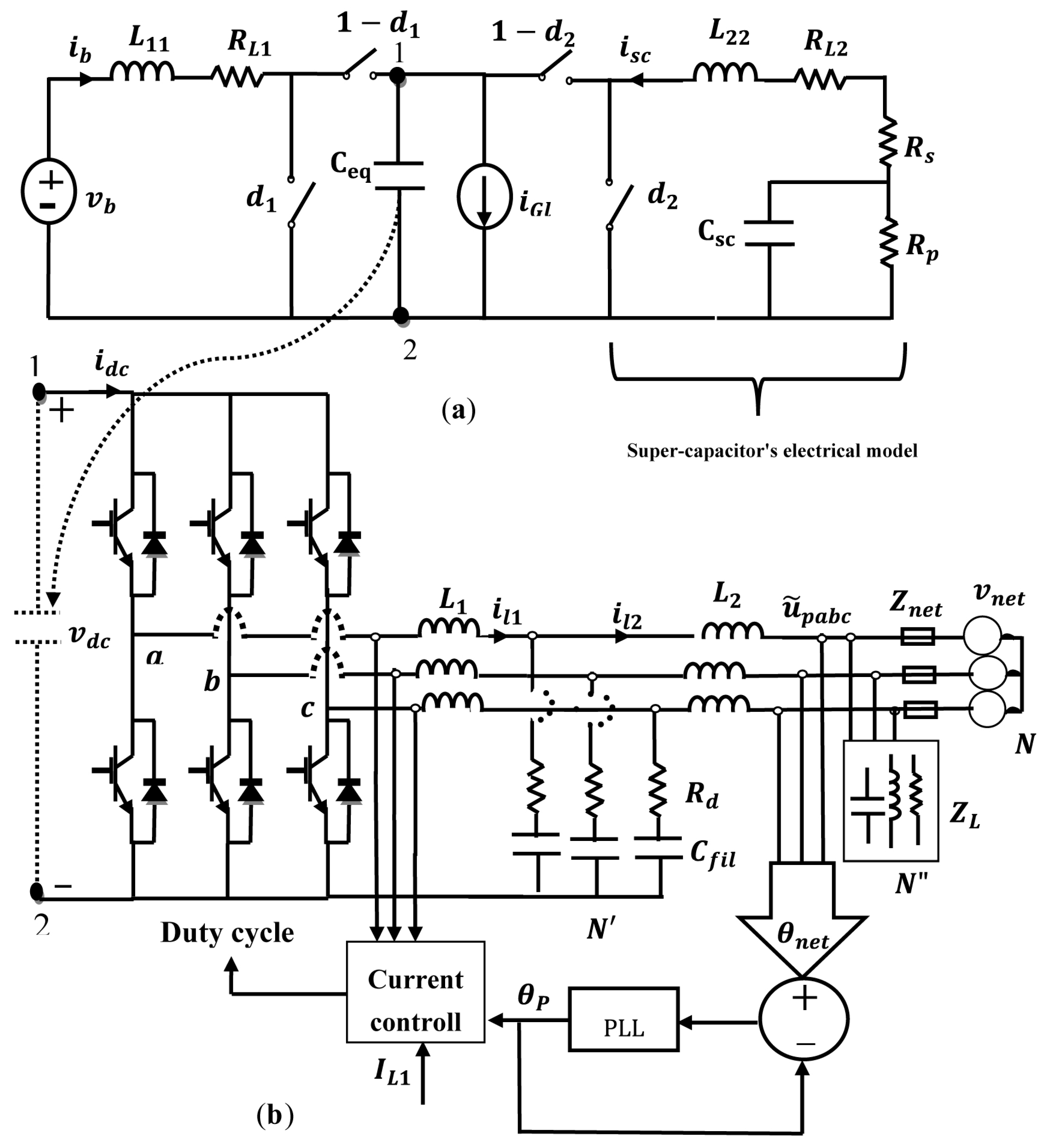
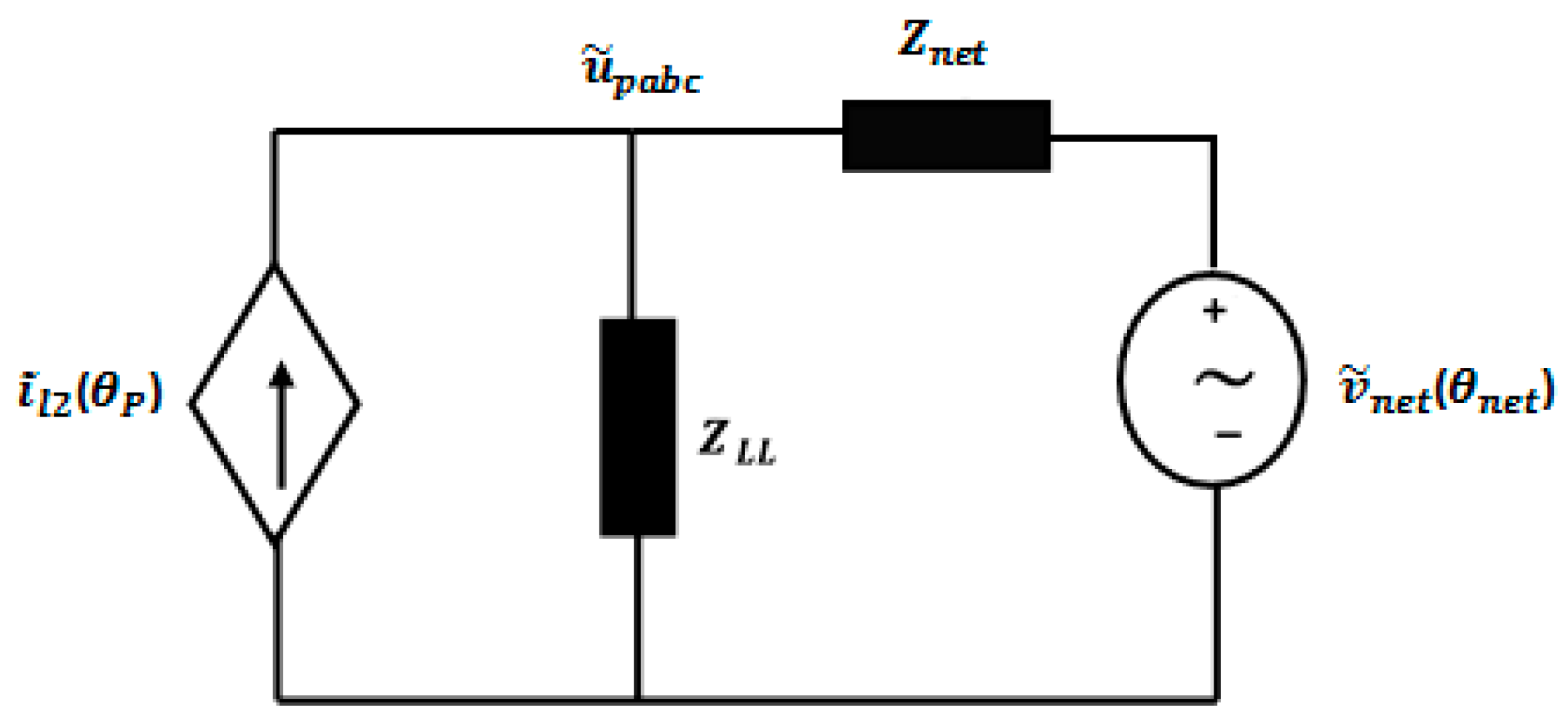
Figure 1, shows the schematic of a micro-grid along with the grid-interface converter. In this Figure, the inverter is connected to the DC bus. The DC bus is modeled with a capacitor with capacitance $C_{eq}$.

In this study, a micro-grid composed of distributed generation sources, a hybrid storage system (batteries and super-capacitors) with a grid -interface bi-directional converter, DC and AC loads, grid-interface converter and energy management system are considered.

Figure 1a, is consist of a hybrid storage system and a current source. This current source represents the Differences between the load current and the current produced by distributed generation sources. Also, Figure 1a, shows the scheme of three phase converter connected to the grid through a LCL filter. (DC bus feeds grid-interface converter in Figure 1a)

In Figure 1, $C_{sc},R_p,R_s,L_{22},L_{11},R_{L2},R_{L1},i_{Gl},Z_L,Z_{net},u_{net},L_1,L_2,C_{fil},R_d,$ are the equivalent capacity of super-capacitor, the equivalent parallel resistance of super-capacitor, the equivalent series resistance of super-capacitor, the filter inductance of super-capacitor’s converter, the filter inductance of battery’s converter, The equivalent resistance of power losses related to the switches of super-capacitor’s converter and the equivalent resistance of power losses related to the switches of battery’s converter, the differences between the load current and the current produced by distributed generation sources, the local load impedance (ohmic load ($R_L$) parallel with inductive load ($L_L$)), the network (grid) impedance, the network (grid) voltage, the inverter-side inductance, the grid-side inductance, the filter capacitance and damping resistor, respectively.

2.1. Hybrid Storage System

A hybrid storage system, consisting of a battery, a super-capacitor and bidirectional power converters is used to maintain the DC bus voltage and to manage the energy of system. Input or output current of storage system can be controlled appropriately. The control system related to the hybrid storage system would be discussed in the next section. By assuming the insignificance of the switching losses and assuming ideal switches, the average model for hybrid storage system can be obtained from the following equations [24]:

$$\frac{d{\overline{i}}_b}{dt}=\frac{1}{L_{11}}({\overline{u}}_b-\left(1-d_1\right){\overline{u}}_{dc}-{\overline{i}}_b{R}_{L1})$$

(1)

$$\frac{d{\overline{i}}_{sc}}{dt}=\frac{1}{L_{22}}({\overline{u}}_{sc}-\left(1-d_2\right){\overline{u}}_{dc}-{\overline{i}}_{sc}{R}_{L2})$$

(2)

$$\frac{d{\overline{u}}_{sc}}{dt}=\frac{1}{C_{sc}}({\overline{u}}_{sc}\left(-\frac{C_{sc}{R}_s}{L_{22}}-\frac{1}{R_p}\right)+{\overline{u}}_{dc}\left(\frac{C_{sc}{R}_s\left(1-d_2\right)}{L_{22}}\right) - {\overline{i}}_{sc}\left(1+\left(\frac{R_s}{R_p}\right)-\frac{C_{sc}{R}_s{R}_{L2}}{L_{22}}\right)$$

(3)

where $u_{sc},u_b,i_{sc},i_b,d_2,d_1$ are the super-capacitor voltage, the battery voltage, the super-capacitor current, the battery current, the duty cycle of super-capacitor’s converter, the duty cycle of battery’s converter, respectively.

2.2. The Controller of Micro-Grid and Grid-Side Converter

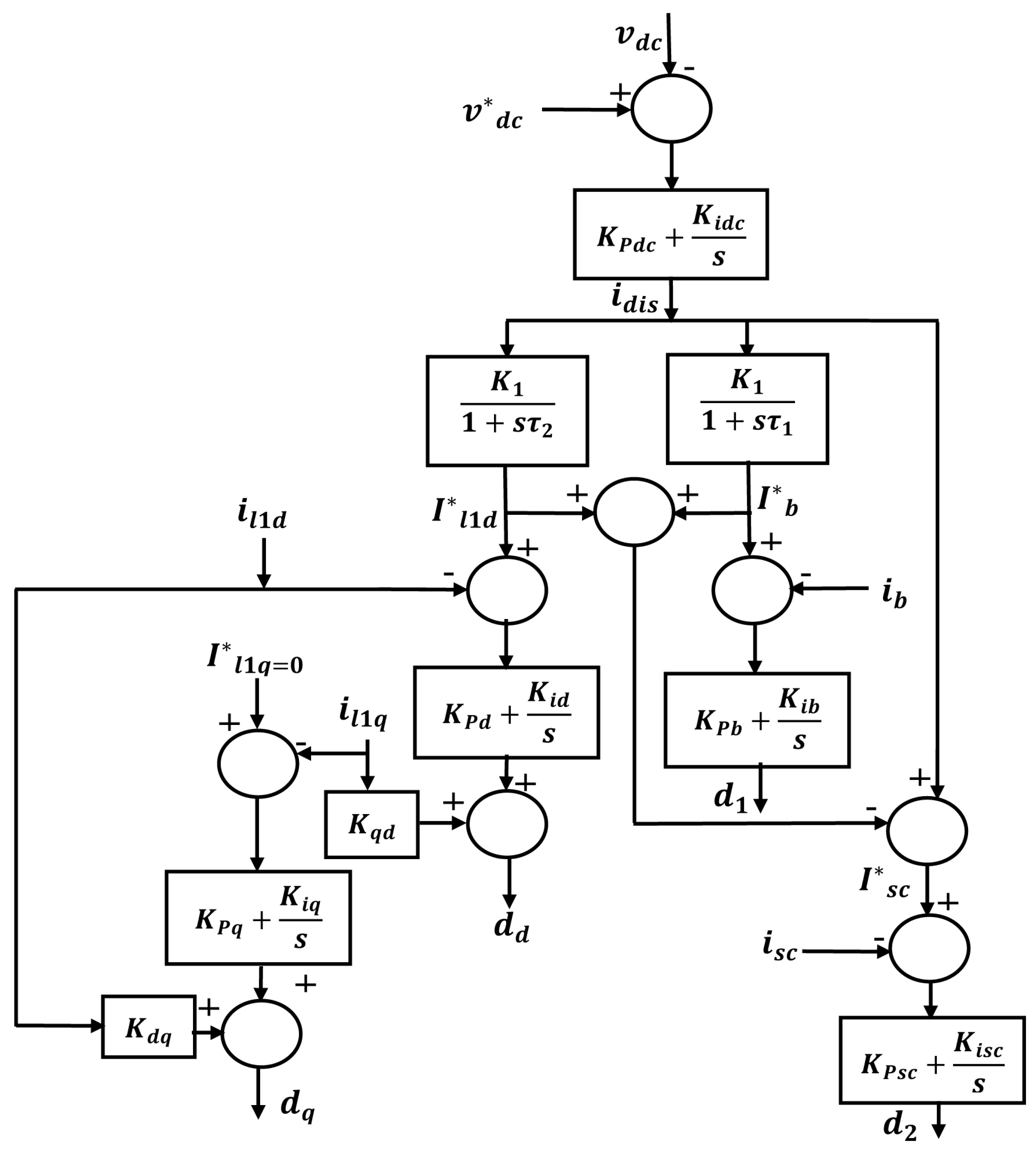
Figure 2 shows the proposed control system that its aim is to maintain the DC bus voltage $u_{dc}$ by regulating the battery, the super-capacitor and the grid-interface converter currents. First, the instantaneous voltage $u_{dc}$ is compared with its reference value. Its error passes from PI controller and the share of the battery, the super-capacitor and the grid-interface converter compensation gets determined. To specify the contribution of each of these elements to the compensation, various indicators could be considered. In this article, sudden changes in power system are compensated by a super-capacitor because, the super-capacitor has a high response speed (super-capacitor employment may also increase battery life). This means that the high frequency error terms would be compensated by the super-capacitor, lower frequency terms by the battery and the rest would be compensated by means of the grid-interface converter.

The so-called frequency bandwidth is determined by a low-pass filter for the battery, a band-pass filter for grid-interface converter and the rest for the grid-interface converter. In this control system, ${\tau }_1,{\tau }_2,I^{\ast }{}_b,I^{\ast }{}_{SC},i_{l1d},I^{\ast }{}_{l1d},i_{l1q},I^{\ast }{}_{l1q}$, $i_{dis},u^{\ast }{}_{dc}$ are the time constant of low-pass filter, the time constant of band-pass filter, the reference charging or discharging current of battery, the reference charging or discharging current of super-capacitor, the inverter d-component current in the inverter-side, the inverter d-component reference current in the inverter-side, the inverter q-component current in the inverter-side, the inverter q-component reference current in the inverter-side, the error current caused by the difference between the instantaneous and reference voltage of DC bus and the reference voltage of DC bus and the reference voltage of DC bus, respectively.

2.3. Small Signal Model of Studied Micro-Grid

According to (4), the small-signal model of system represents the amount of fluctuations of average variables around the operating point. In this Equation, the order of $X,\tilde{x},\overline{x}$ is the amount of average variable at the operating point, the small signal term of average variable and the average variable, respectively.

$$\overline{x}=X+\tilde{x}$$

(4)

Applying Equation (4) to all of the Equations corresponding to micro-grid’s components (Due to the large number of the micro-grid’s equations, the details have been ignored) and assume that the small signal term of the average variables and the changes of average variables (derivatives) at the operating point are insignificant, the network operating point would be achieved by solving the Equations. Due to nonlinearity of the average model, the obtained average model equations should be linearized around the operating point. The above linearization process will result in state Equations (5)–(9):

$$\frac{d\tilde{x}\left(t\right)}{dt}=A\tilde{x}\left(t\right)+B\tilde{u}\left(t\right)$$

(5)

$$\tilde{y}\left(t\right)=C\tilde{x}\left(t\right)+D\tilde{u}\left(t\right)$$

(6)

$$\tilde{x}\left(t\right)=\left[{\tilde{i}}_{b,}{\tilde{i}}_{sc},{\tilde{u}}_{dc},{\tilde{i}}_{l1d},{\tilde{i}}_{l1q},{\tilde{i}}_{l2d},{\tilde{i}}_{l2q},{\tilde{i}}_{LLd},{\tilde{i}}_{LLq},{\tilde{u}}_{cfild},{\tilde{u}}_{cfilq},{\tilde{u}}_{sc,}{\tilde{u}}_{pd,}{\tilde{u}}_{pq},\tilde{C},{\tilde{\theta }}_P\right]$$

(7)

$$\tilde{y}\left(t\right)=\left[{\tilde{i}}_{b,}{\tilde{i}}_{sc},{\tilde{u}}_{dc},{\tilde{i}}_{l1d},{\tilde{i}}_{l1q},{\tilde{i}}_{l2d},{\tilde{i}}_{l2q},{\tilde{u}}_{sc,}{\tilde{u}}_{pd,}{\tilde{u}}_{pq},\tilde{C},{\tilde{\theta }}_P\right]$$

(8)

$$\tilde{u}\left(t\right)=\left[{\tilde{d}}_1,{\tilde{d}}_2,{\tilde{d}}_d,{\tilde{d}}_q,{\tilde{u}}_{netd},{\tilde{u}}_{netq},i_{Gl}\right]$$

(9)

In the above Equations, $\tilde{x}\left(t\right)$, $\tilde{y}\left(t\right),$ $\tilde{u}$ are the network state variable, the output vector and the input vector, respectively.

In this regard, the order of ${\tilde{i}}_{l2d},{\tilde{i}}_{l2q},d_d,d_q,{\tilde{i}}_{LLd},{\tilde{i}}_{LLq},{\tilde{u}}_{netd},{\tilde{u}}_{netq},{\tilde{u}}_{cfild},{\tilde{u}}_{cfilq},{\tilde{u}}_{pd,}{\tilde{u}}_{pq},\tilde{C},{\tilde{\theta }}_P$ are the inverter d-component current in the grid-side, the inverter q-component current in the grid-side, the d-component duty cycle of grid-interface converter, the q-component duty cycle of grid-interface converter, the d-component instantaneous current of local load, the q-component instantaneous current of local load, the d-component instantaneous voltage of network, the q-component instantaneous voltage of network, the d-component instantaneous voltage of filter capacitor, the q-component instantaneous voltage of filter capacitor, the d-component voltage measured by PLL, the q-component voltage measured by PLL, the angle of inverter current in the grid-side inverter.

3. Proposed Criteria for the Stability Analysis of PLL

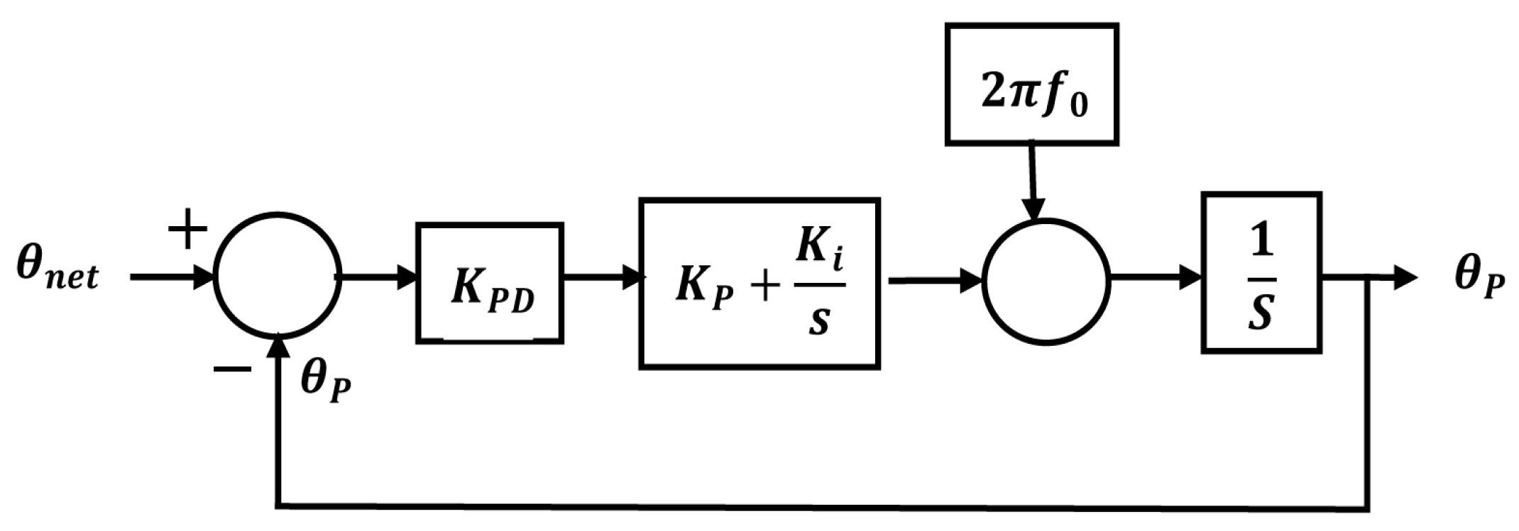
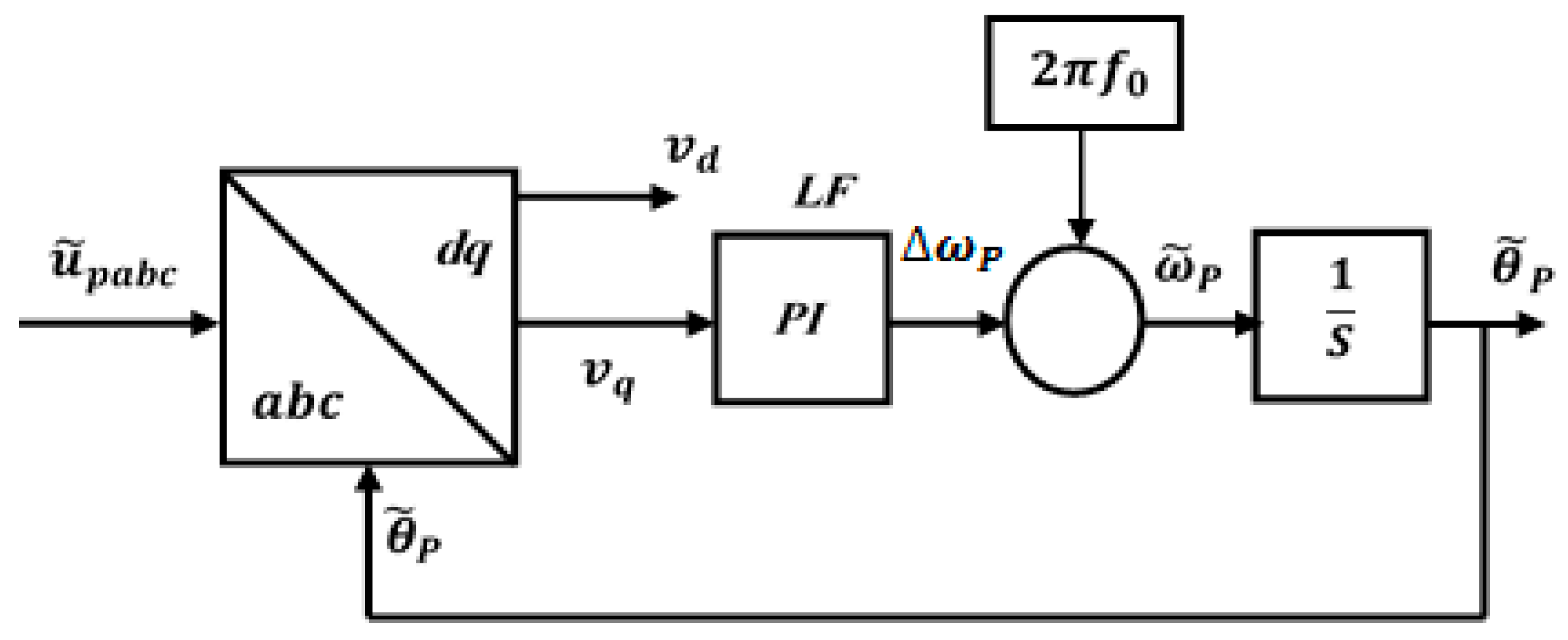
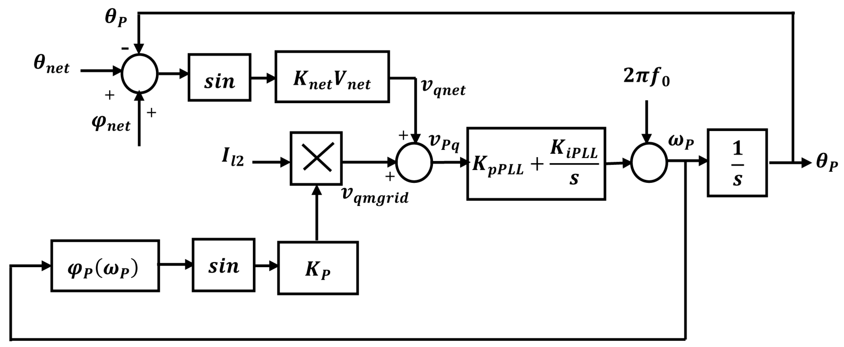
Almost all PLLs are comprised of three basic parts: phase detector (PD), loop filter (LF) and voltage controlled oscillator (VCO) [5]. Figure 3, shows the overall structure of a conventional SRF-PLL. The phase angle of input signal is compared with the feedback of the output of oscillator and the error signal is produced proportional to the difference between the input and output phase angles. Phase detector output, consists of harmonic components, passed by the low-pass filter. Controlled output voltage of the loop filter (which is a function of frequency) enters into the oscillator and produces a phase output. The output signal (which is in the form of phase angle) goes back to the phase detector with a negative feedback. The output signal of oscillator is compared with the input; if their frequency were different, the output frequency of oscillator is changed to be equal with the input frequency. In this PLL, as seen in Figure 4, a three-phase input voltage (${\tilde{u}}_{pabc}$) is transformed into the rotating frame ($u_{pd}, u_{pq}$) using Clarke and Park transformation.

Using a feedback loop, the angular position of dq framework is controlled in a way that one of the d or q voltage components is zero. Assuming that the network voltage ${\tilde{u}}_{net}$(${\theta }_{net}$) is a vector that is rotating with a synchronous angle ${\theta }_{net}$, hence the angle ${\theta }_P$ must match the angle ${\theta }_{net}$ to synchronize the inverter’s output current with network voltage.

According to the Park transformation matrix:

$$\left[\begin{array}{c}{u}_{pd}\\ u_{pq}\\ u_{p0}\end{array}\right]=\frac{2}{3}\left[\begin{array}{c}\cos \left({\theta }_p\right) \cos ({\theta }_p-\frac{2\pi }{3}) \cos ({\theta }_p+\frac{4\pi }{3})\\ \sin \left({\theta }_p\right) \sin ({\theta }_p-\frac{2\pi }{3}) \sin ({\theta }_p+\frac{4\pi }{3})\\ \frac{1}{2} \frac{1}{2} \frac{1}{2}\end{array}\right]\left[\begin{array}{c}{u}_{net}\cos \left({\theta }_{net}\right)\\ u_{net}\cos ({\theta }_{net}-\frac{2\pi }{3})\\ u_{net}\cos ({\theta }_{net}+\frac{2\pi }{3})\end{array}\right]$$

(10)

$$u_{pq}=u_{net}\sin \left({\theta }_{net}-{\theta }_P\right)$$

(11)

According to the Equation (11), to match angle ${\theta }_P$ on the angle ${\theta }_{net}$, the $u{p}_q$ must be equal to zero. It should be noted that this compliance, in addition to maintaining synchronization between the output voltage of micro-grid and the voltage of main network will also contribute to the stability of PLL. (Because $u{p}_q$ enters into the integrator, its non-zero value may lead to instability of PLL.) Therefore, the condition $u{p}_q=0$ is considered to be as a proposed criterion for the stability of the PLL.

According to the Equation (6), the output current of inverter ${\tilde{i}}_{l2}$(${\theta }_P$) has two components ${\tilde{i}}_{l2q}$ and ${\tilde{i}}_{l2d}$ that be obtained as follows:

$${\tilde{i}}_{l2d}=C_{61}·{\tilde{i}}_b+C_{62}·{\tilde{i}}_{sc}+\cdots +C_{616}·{\tilde{\theta }}_P+ D_{61}·{\tilde{d}}_1+D_{62}·{\tilde{d}}_2+\cdots +D_{67}·i_{Gl}$$

(12)

$${\tilde{i}}_{l2q}=C_{71}·{\tilde{i}}_b+C_{72}·{\tilde{i}}_{sc}+\cdots +C_{716}·{\tilde{\theta }}_P+D_{71}·{\tilde{d}}_1+D_{72}·+\cdots +D_{77}·i_{Gl}$$

(13)

The order of $C_{61},C_{62},\dots ,C_{716},D_{61},D_{62},\dots D_{77}$ are the elements of matrices C and D in state equations. According to the above relations and considering that output current of inverter is a vector, this current can be showed as follows:

$${\tilde{i}}_{l2}({\theta }_P)=I_{l2}{e}^{j{\theta }_P}$$

(14)

$$I_{l2}=\sqrt{\left({\left|{\tilde{i}}_{l2d}\right|}^2+{\left|{\tilde{i}}_{l2q}\right|}^2\right)}$$

(15)

In Equation (14), $I_{l2}$ and ${\theta }_P$ are the amplitude and the angle of output current of inverter, respectively. This angle was determined by the PLL. In Figure 5, it is assumed that the PLL position is after the inverter LCL filter. In this case, the voltage which the PLL measures (${\tilde{u}}_{pabc}$) is affected by two factors: the network-side parameters and the micro-grid-side parameters. Also, it is assumed that $Z_{net}$ and ${\tilde{u}}_{net}$(${\theta }_{net}$) are the impedance and the voltage of the network, respectively. Therefore, the input voltage to the PLL will be as follows:

$${\tilde{u}}_{pabc}={\tilde{u}}_{mgrid}+{\tilde{u}}_{net}$$

(16)

In this regard, the order of ${\tilde{u}}_{net}$ and ${\tilde{u}}_{mgrid}$ is the voltage caused by network-side factors connected to the Micro-grid (the main grid) and the voltage caused by microgrid-side factors, respectively. As shown in Figure 5.

$${\tilde{u}}_{mgrid}={\tilde{i}}_{l2}\left({\theta }_P\right)·\frac{Z_L{Z}_{net}}{Z_L+Z_{net}} = \sqrt{\left({\left|{\tilde{i}}_{l2d}\right|}^2+{\left|{\tilde{i}}_{l2q}\right|}^2\right)}\left|\frac{Z_L{Z}_{net}}{Z_L+Z_{net}}\right|e^{j\left({\theta }_P+{\phi }_P\right)}$$

(17)

$${\phi }_P=Phase \left(\frac{Z_L{Z}_{net}}{Z_L+Z_{net}}\right)$$

(18)

$${\tilde{u}}_{net}={\tilde{u}}_{net}\left({\theta }_{net}\right)·\frac{Z_L}{Z_L+Z_{net}}=\left|{\tilde{u}}_{net}\right|\left|\frac{Z_L}{Z_L+Z_{net}}\right|e^{j\left({\theta }_{net}+{\phi }_{net}\right)}$$

(19)

$${\phi }_{net}=Phase \left(\frac{Z_L}{Z_L+Z_{net}}\right)$$

(20)

In above Equations, $Z_L$, $Z_{net}$, ${\phi }_{net}$ and ${\phi }_P$ are the local load impedance, the network impedance, the phase created by the existence of the network and load impedances in network frequency and the phase created by the existence of the network and load impedances in output angular frequency of PLL $\left({\omega }_P\right)$, respectively.

$$K_{net}\left({\omega }_{net}\right)=\left|\frac{Z_L\left({\omega }_{net}\right)}{Z_L\left({\omega }_{net}\right)+Z_{net}\left({\omega }_{net}\right)}\right|$$

(21)

$${\mathsf{\phi }}_{net}\left({\omega }_{net}\right)=Phase(\frac{Z_L\left({\omega }_{net}\right)}{Z_L\left({\omega }_{net}\right)+Z_{net}\left({\omega }_{net}\right)})$$

(22)

$$K_P\left({\omega }_P\right)=\left|\frac{Z_L\left({\omega }_P\right)Z_{net}\left({\omega }_P\right)}{Z_L\left({\omega }_P\right)+Z_{net}\left({\omega }_P\right)}\right|$$

(23)

$${\mathsf{\phi }}_P\left({\omega }_P\right)=Phase(\frac{Z_L\left({\omega }_P\right)Z_{net}\left({\omega }_P\right)}{Z_L\left({\omega }_P\right)+Z_{net}\left({\omega }_P\right)})$$

(24)

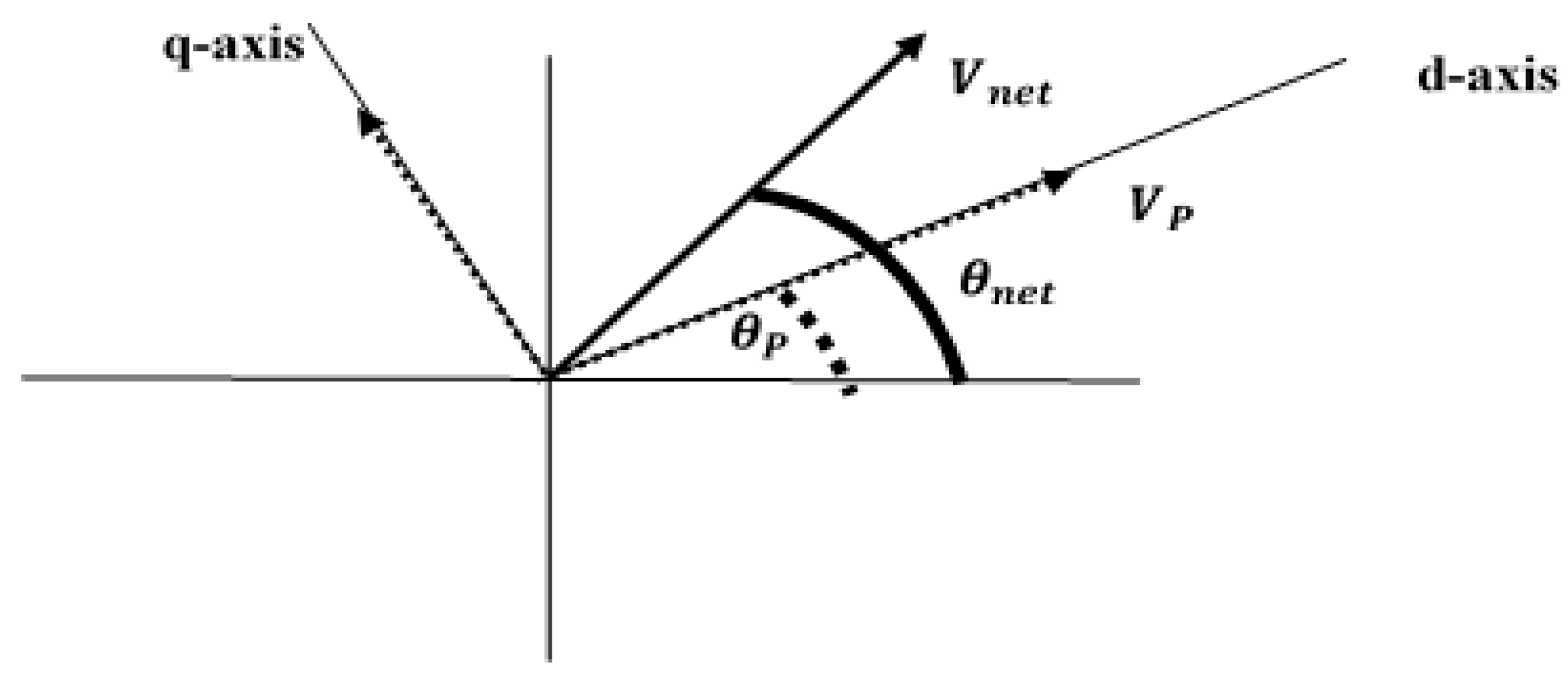
Assuming that the network voltage ${\tilde{u}}_{net}$(${\theta }_{net}$), is a vector that is spinning with a synchronous angle ${\theta }_{net}$, the angle ${\theta }_P$ be coincident on the angle ${\theta }_{net}$ to make the output current of inverter synchronized with the network voltage. (Details is in Figure 6)

According to the Park transformation matrix:

According to the Equation (11), to match angle ${\theta }_P$ on the angle ${\theta }_{net}$, the $u_q$ must be equal to zero. It should be noted that this compliance, in addition to maintaining synchronization between the output voltage of micro-grid and the voltage of main network, will also contribute to the stability of PLL (Because $u_q$ enters into the integrator, its non-zero value may lead to instability of PLL). Based on Equations (17), (19) and Figure 7, $u_{Pq}$ has two parts of $u_{qnet}$ and $u_{qmgrid}$ which are affected by the main network-side parameters and the microgrid- side parameters, respectively. In fact, it can be said that part $u_{qmgrid}$ is a kind of annoying factor for the PLL that tries to help ${\theta }_P$ get away from ${\theta }_{net}$. The remarkable thing about Equation (25) (annoying factor for the PLL stability) is that the amplitude and direction of inverter’s output current, the local load type and the size of main network impedance may influence the PLL stability.

$$v_{qmgrid}=I_{l2}·\sin \left({\phi }_P\left({\omega }_P\right)\right)·K_P$$

(25)

Moreover, the part related to the main network-side parameters ($u_{qnet}$), tries to neutralize the effectiveness of micro-grid-side factors by setting of ${\phi }_{net}+{\theta }_{net}-{\theta }_P$. Considering that the maximum amount of $u_{qnet}$ is equal to $K_{net}{u}_{net}$, then if the amplitude of $u_{qmgrid}$ is more than the maximum amount of $u_{qnet}$, no ${\theta }_P$ would be found to make $u_q$ zero; this can disturb the stability of the PLL. Therefore, with regard to aforementioned, another stability index may be achieved for PLL as following:

PLL is stable if:

$$\left|u_{qmgrid}\right|<\left|u_{qnet}\right|$$

(26)

$$I_{l2}<\frac{\left|u_{net}·K_{net}\right|}{\left|\sin \left({\phi }_P\left({\omega }_P\right)\right)·K_P\right|}$$

(27)

Therefore, in this section, two stability criteria ($u{p}_q=0$ and Equation (27)) for the PLL were obtained and in the next section, according to the mentioned stability criteria, the stability of PLL affected by network-side and grid-side factors would be examined.

4. Determining the Optimal Parameters of the Studied Micro-Grid by Taguchi Method

The Optimization Process is one of the most important activities in today’s competitive industry. The high cost of research and development projects has necessitated the exploitation of experiment design methods to determine the impressive factors on processes with the least number of tests. Methods of experiment design have widely been used in the past two decades to achieve this goal. Compared with other commonly-used methods such as full factorial design, fractional factorial, Latin Squares, etc., Taguchi experimental design method, in addition to having this role, has found much wider applicability because of being more comprehensive in some parts of the industry [25]. Taguchi method may be considered as a statistical method to optimize and improve the quality of each process.

In some cases, the traditional experimental designs are very complicated and sometimes infeasible. When the number of parameters in a process is large, a great number of experiments (simulations) are required to optimize the parameters of the experimental design method. Taguchi method uses a specific orthogonal array to resolve this problem and investigate all parameters by using a few tests (simulations). Taguchi method is widely used in engineering analysis with the aim of obtaining information about the behavior of a process [26,27,28,29,30]. The biggest advantages of this method include saving the number of experiments (simulations), saving the time, reducing the costs, etc.

4.1. Testing and Analysis

The purpose of the study is to evaluate the effects of the micro-grid and hybrid storage system parameters on the stability of PLL. The study simultaneously aimed at determining the optimal values of these parameters to improve the stability of PLL and thereby improve the stability of the network-side converter. For this purpose, $C_{eq},L_{11},C_{sc}{L}_{22},i_{Gl},\tau ,L_2,L_1,C_f,R_L,L_L,z_{net}$ are considered as micro-grid electrical parameters and $z_{net}$ as the main network parameter. In contrast, $u{p}_q=0$ is determined as proposed PLL stability criterion and it is considered as the most important characteristic of the output process. Each regulatory parameter (micro-grid and network-side parameters) has been evaluated in three levels.

Table 1. Different levels of process variables.

Parameter	$\mathbf{L}\mathbf{e}\mathbf{v}\mathbf{e}\mathbf{l} 1$	$\mathbf{L}\mathbf{e}\mathbf{v}\mathbf{e}\mathbf{l} 2$	$\mathbf{L}\mathbf{e}\mathbf{v}\mathbf{e}\mathbf{l} 3$
$L_{11}$	$0.1\mathrm{mH}$	$1\mathrm{mH}$	$10\mathrm{mH}$
$L_{22}$	$0.1\mathrm{mH}$	$1\mathrm{mH}$	$10\mathrm{mH}$
$C_{sc}$	$0.1\mathrm{F}$	$1\mathrm{F}$	$3\mathrm{F}$
$C_{eq}$	$0.1\mathrm{mF}$	$1\mathrm{mF}$	$10\mathrm{mF}$
$L_1$	$45\mathsf{\mu }\mathrm{H}$	$70\mathsf{\mu }\mathrm{H}$	$100\mathsf{\mu }\mathrm{H}$
$\tau$	$0.50\mathrm{s}$	$5\mathrm{s}$	$10$s
$R_L$	$2\Omega$	$5\Omega$	$10\Omega$
$L_2$	$45\mathsf{\mu }\mathrm{H}$	$70\mathsf{\mu }\mathrm{H}$	$100\mathsf{\mu }\mathrm{H}$
$C_{fil}$	$40\mathsf{\mu }\mathrm{F}$	$60\mathsf{\mu }\mathrm{F}$	$100\mathsf{\mu }\mathrm{F}$
$Z_{net}$	$10\Omega$	$40\Omega$	$90\Omega$
$L_L$	$30\mathrm{mH}$	$50\mathrm{mH}$	$70\mathrm{mH}$
$i_{Gl}$	− $50\mathrm{A}$	− $60\mathrm{A}$	− $80$A

shows the regulatory parameters of the process along with their levels.

To achieve the aims of this study, a set of simulations data related to the process is required. According to the number of parameters and their levels, the total number of states (tests or simulations) is obtained from $n=L^K$. In this equation, n is the number of experiments, L is the number of levels and K is the number of considered parameters. In this study, there are 12 parameters in each of the 3 levels. Therefore, the total number of simulations will be equal to 531,441 tests (simulations). It is clear that carrying out this large number of tests is very time consuming. Moreover, it is not cost-effective. Therefore, Taguchi experimental design approach is used to collect the required data. Taguchi provides a practical approach regarding the quality control of manufacturing industries.

The main objectives of Taguchi method include determining the effect of each parameter on the output process and determining the optimal levels of these parameters. Taguchi method achieves these goals by analyzing simulations data which have been collected in predetermined terms. In this study, experiments have been designed by Minitan17 software. Taguchi suggests an $L_{27}$ orthogonal array for 12 input factors and 3 levels.

Resultantly, 27 simulative tests were performed according to the levels shown in

Table 2. Output result of simulation for measurement of $v_{pq}$ .

Simulation Number	${\mathit{L}}_1$	${\mathit{L}}_2$	${\mathit{L}}_{11}$	${\mathit{L}}_{22}$	${\mathit{C}}_{\mathit{e}\mathit{q}}$	${\mathit{C}}_{\mathit{f}\mathit{i}\mathit{l}}$	${\mathit{R}}_{\mathit{L}}$	${\mathit{L}}_{\mathit{L}}$	${\mathit{C}}_{\mathit{s}\mathit{c}}$	${\mathit{Z}}_{\mathit{n}\mathit{e}\mathit{t}}$	$\mathit{\tau }$	${\mathit{i}}_{\mathit{G}\mathit{l}}$	${\mathit{v}}_{\mathit{p}\mathit{q}}$	$\raisebox{1ex}{$\mathit{S}$}\!\left/ \!\raisebox{-1ex}{$\mathit{N}$}\right.$
1	1	1	1	1	1	1	1	1	1	1	1	1	$0.0714$	$18.5776$
2	1	1	1	1	2	2	2	2	2	2	2	2	$0.2857$	$09.8591$
3	1	1	1	1	3	3	3	3	3	3	3	3	$0.5000$	$06.0206$
4	1	2	2	2	1	1	1	2	2	2	3	3	$0.1176$	$17.1272$
5	1	2	2	2	2	2	2	3	3	3	1	1	$0.3319$	$08.9442$
6	1	2	2	2	3	3	3	1	1	1	2	2	$0.2184$	$12.2950$
7	1	3	3	3	1	1	1	3	3	3	2	2	$0.1638$	$14.7938$
8	1	3	3	3	2	2	2	1	1	1	3	3	$0.0504$	$20.0000$
9	1	3	3	3	3	3	3	2	2	2	1	1	$0.2647$	$10.8818$
10	2	1	2	3	1	2	3	1	2	3	1	2	$0.3025$	$09.0329$
11	2	1	2	3	2	3	1	2	3	1	2	3	$0.2268$	$12.0412$
12	2	1	2	3	3	1	2	3	1	2	3	1	$0.1260$	$15.7031$
13	2	2	3	1	1	2	3	2	3	1	3	1	$0.0840$	$18.3156$
14	2	2	3	1	2	3	1	3	1	2	1	2	$0.2731$	$10.2544$
15	2	2	3	1	3	1	2	1	2	3	2	3	$0.1848$	$13.9795$
16	2	3	1	2	1	2	3	3	1	2	2	3	$0.2815$	$09.8699$
17	2	3	1	2	2	3	1	1	2	3	3	1	$0.0294$	$22.1026$
18	2	3	1	2	3	1	2	2	3	1	1	2	$0.1176$	$16.9054$
19	3	1	3	2	1	3	2	1	3	2	1	3	$0.2689$	$10.4574$
20	3	1	3	2	2	1	3	2	1	3	2	1	$0.1680$	$14.0500$
21	3	1	3	2	3	2	1	3	2	1	3	2	$0.0924$	$18.0618$
22	3	2	1	3	1	3	2	2	1	3	3	2	$0.1638$	$14.1372$
23	3	2	1	3	2	1	3	3	2	1	1	3	$0.2521$	$11.2133$
24	3	2	1	3	3	2	1	1	3	2	2	1	$0.0040$	$49.1186$
25	3	3	2	1	1	3	2	3	2	1	2	1	$0.0966$	$17.8219$
26	3	3	2	1	2	1	3	1	3	2	3	2	$0.0084$	$30.9031$
27	3	3	2	1	3	2	1	2	1	3	1	3	$0.1974$	$13.0964$

and the amount of $u_{Pq }$ was measured through the simulation of the mentioned micro-grid (Figure 1) in MATLAB software. The measured value of $u_{Pq}$ is provided in column 14 in Table 2.

4.2. The Signal to Noise Ratio Analysis

Signal to noise ratio, represents the sensitivity of the studied characteristic to Input factors in a controlled process [27,28,29,30,31]. The optimum condition is detected by determining the effect of each input factor on output Characteristic. From the perspective of the characteristic of the output process, it can be divided into three categories: the less is the better (smaller is better), the closer to nominal amount is the better (nominal is better) and the bigger is the better (larger is better). Taguchi has offered different equations to calculate the signal to noise ratio in terms of the relevance of the desired Characteristic to any of the three mentioned groups [25,32]. In general, the highest ratio (S/N) is always desirable in each test. The output measured in this study is $u_{Pq}$ which is placed in the category the smaller is better. Therefore, the following equation is used to calculate the signal to noise ratio.

$$\frac{S}{N}=-10 {log}_{10}\left(\frac{1}{n}{{\displaystyle \sum }}_{i=1}^n{\left(y_i\right)}^2\right)$$

(28)

In above equation, n is the frequency of each test and $y_i$ is i-th measured output. Signal to noise ratio is calculated for each of the 27 experiments performed using the equation mentioned above and is shown in the last column in Table 2. In this study, each of the tests was done only once and thus, n is equal to one.

4.3. Analysis of Results for Determining of Optimal Parameters

Because in the Taguchi experiments, only some parts of the possible cases are tested, to ensure the accuracy of the final results, appropriate statistical methods should be used. Analysis of variance is a statistical method that calculates the degree of confidence and determines the contribution percentage of each variable on the output process. Then, the statistical analysis conducted on the results of the experiments (simulations) in micro-grid for the PLL stability are provided.

Table 3. Result of analysis of variance of signal to noise ratio.

Parameter	DF	Adj SS	Adj MS	F Value	p Value	p (%)
$R_L$	2	0.03144	0.015721	4.32	0.039	8.05
$L_1$	2	0.03845	0.019224	5.28	0.023	10.25
$\tau$	2	0.04537	0.022686	6.23	0.014	12.04
$L_L$	2	0.05327	0.026634	7.32	0.008	14.03
$C_{eq}$	2	0.03845	0.019224	5.28	0.023	10.25
$i_{Gl}$	2	0.04576	0.022882	6.29	0.013	12.16
$C_{sc}$	2	0.04535	0.022675	6.23	0.014	12.04
$Z_{net}$	2	0.03846	0.019229	4.56	0.034	9.03
$C_{fil}$	2	0.001634	0.000817	2.40	0.294	4.35
$L_2$	2	0.000670	0.000335	0.98	0.504	1.84
$L_{22}$	2	0.000493	0.000246	0.72	0.58	1.32
$L_{11}$	2	0.000591	0.000301	0.87	0.510	1.52
$Error$	2	0.03667	0.003056	-	-	3.12
$Total$	26	0.376196	-	-	-	100

, shows the analysis of variance for q-axis component of the voltage measured by the PLL ($u_{Pq}$). This analysis has been carried out based on a confidence level of 95% (uncertainty 5%).

Columns 2–7 in the Table 3 show the degrees of freedom (DF) for each parameter, the sum of squares (seq SS), the adjusted sum of squares (Adj SS), the average sum of squares (Adj MS), F statistic, p statistic and the effect of each input parameter on the desired output (p%), respectively. p statistics is used to determine the significant influence of each parameter on the output. According to the analysis which was based on 95% confidence level, if p value for each parameter is less than 0.05, it would be indicative of the significant influence of each parameter on the output. As is shown in the Table 3, p value is less than 0.05 for some parameters.

Table 3, shows the effect of each micro-grid and main grid parameter on the q-axis component of the voltage measured by the PLL ($u_{Pq}$) and thus the stability of PLL. It is clear that the inductive local load (with inductance $L_L$) has the greatest impact on the stability of PLL by more than 14 percent. Other parameters are in order of importance $i_{Gl},\tau ,C_{sc},L_1,C_{eq},z_{net},R_L,C_{fil},L_2,L_{11},L_{22}$. In the present study, the amount of signal to noise (S/N) was calculated for the results of all the tests using Equation (28). Then, the mean value of the signal to noise ratio was obtained for each level of each parameter tested. 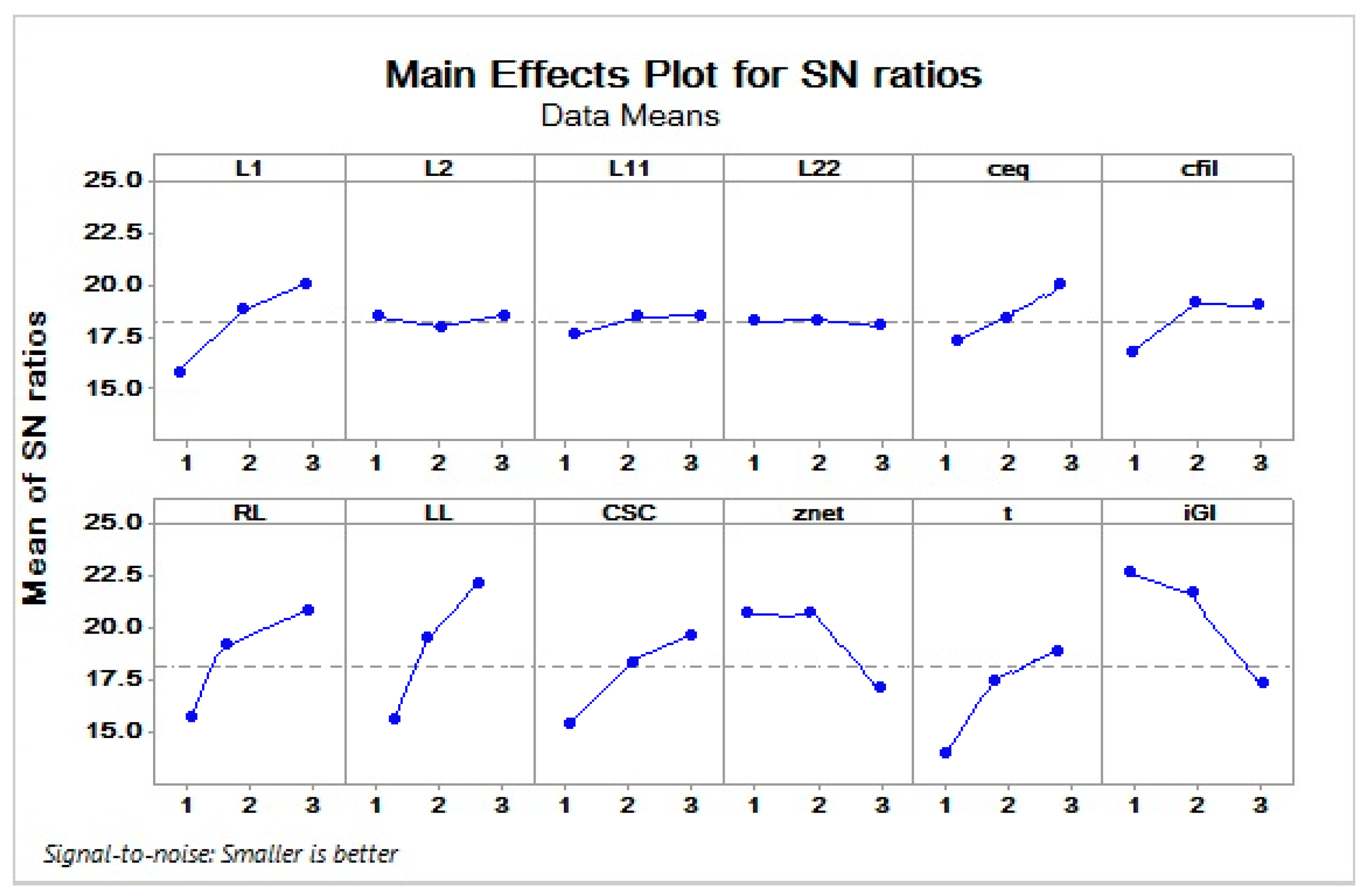Figure 8, shows the mean signal to noise ratio for each of the 12 adjustment parameters in the $u_{Pq}$. As mentioned earlier, high levels of signal to noise ratio are always desirable. Therefore, based on the mean signal to noise ratio of each adjustment parameter, it is possible to determine their optimal levels. According to Figure 6, the best levels for the parameters of the micro-grid and network to achieve the best stability of the grid-side converter and the PLL stability is in

Table 4. Optimal levels for micro-grid and network parameters to achieve the best stability of the PLL.

Parameter	Level	Optimal Value
$L_{11}$	$3$	$10\mathrm{mH}$
$L_{22}$	1	$0.1 \mathrm{mH}$
$C_{sc}$	3	$3 \mathrm{F}$
$C_{eq}$	$3$	$10\mathrm{mF}$
$L_1$	$3$	$100 \mathsf{\mu }\mathrm{H}$
$\tau$	$3$	$10$s
$R_L$	3	$10\Omega$
$L_2$	$3$	$100 \mathsf{\mu }\mathrm{H}$
$C_{fil}$	3	$100\mathsf{\mu }\mathrm{F}$
$Z_{net}$	1	$10\Omega$
$L_L$	3	$70\mathrm{mH}$
$i_{Gl}$	1	$-20 \mathrm{A}$

.

According to the Result of variance analysis of signal to noise ratio (Table 3) and mean of signal to noise ratio (Figure 8), it is clear that the inductive local load (with inductance $L_L$) has the greatest impact on the stability of PLL by more than 14 percent. Other parameters are in order of importance $i_{Gl},\tau ,C_{sc},L_1,C_{eq},z_{net},R_L,C_{fil},L_2,L_{11},L_{22}$. The eigenvalues of micro-grid’s state matrix (in Equation (5)) for the optimal values of micro-grid parameters are given in

Table 5. Eigenvalues of micro-grid’s state matrix for optimal values of micro-grid parameters.

State Variables	Eigenvalues
${\tilde{i}}_b$	−32.91 + 26.07i
${\tilde{i}}_{sc}$	−18.72 + 10.00i
${\tilde{u}}_{dc}$	−131.62 − 100.34i
${\tilde{i}}_{l1d}$	−131.62 + 100.34i
${\tilde{i}}_{l1q}$	−150.06 − 95.87i
${\tilde{i}}_{l2d}$	−150.06 + 95.87i
${\tilde{i}}_{l2q}$	−99.05
${\tilde{i}}_{LLd}$	−185.13
${\tilde{i}}_{LLq}$	−245.95
${\tilde{u}}_{cfild}$	−15.53 − 37.12i
${\tilde{u}}_{sc}$	−15.53 + 37.12i
${\tilde{u}}_{pd}$	−2.32 − 10.48i
${\tilde{u}}_{pq}$	−2.32 + 10.48i
$\tilde{C}$	−85.12 − 38.14i
${\tilde{\theta }}_P$	−85.12 + 38.14i

.

The indicated Eigenvalues in Table 5 show that the studied micro-grid and also the PLL of grid-interface converter are stable for the micro-grid’s optimal parameters.

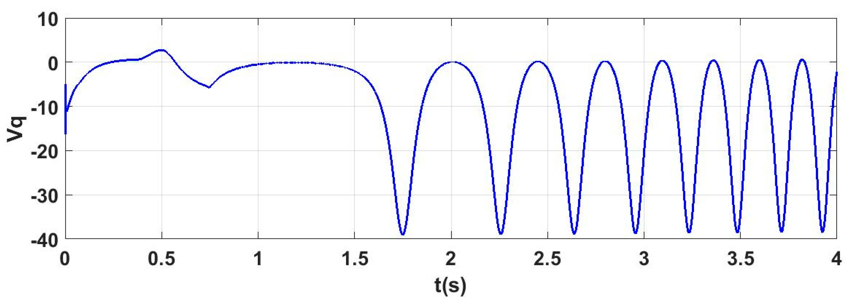
Also, for confirmation of the obtained results from the analysis of the Eigenvalues and the proposed stability criteria of PLL, the studied micro-grids simulated for optimal values of micro-grid and network parameters.

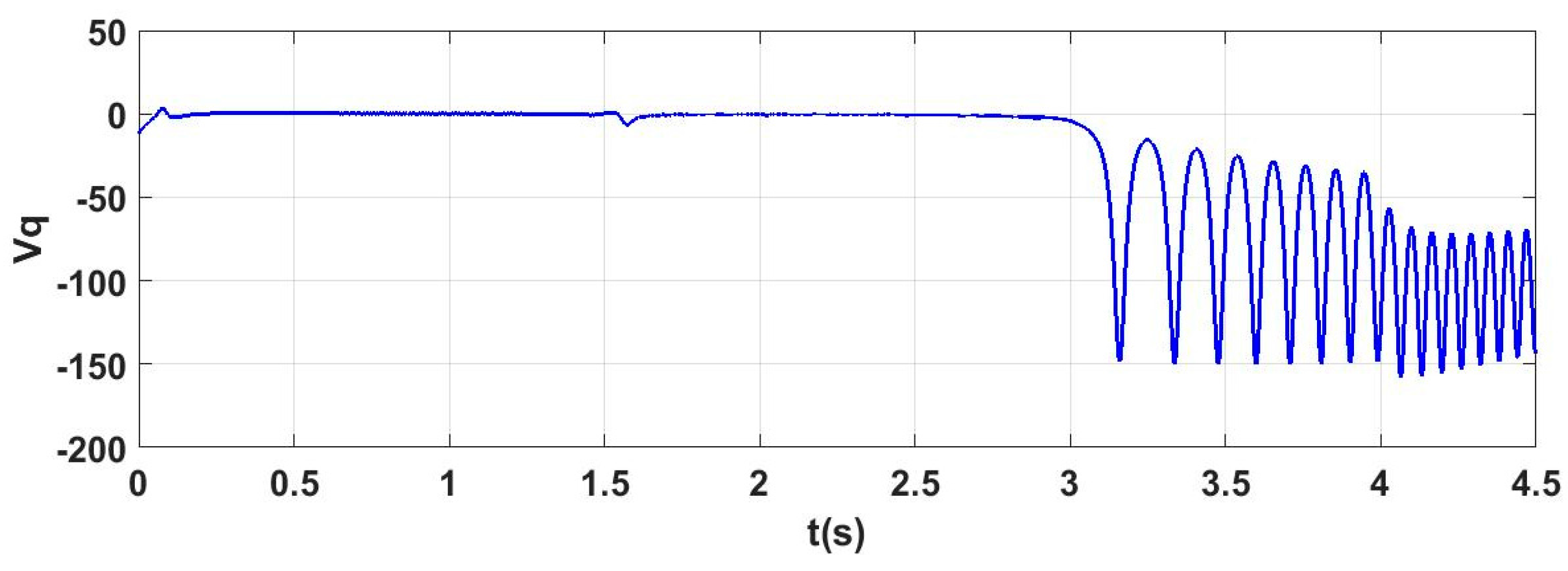
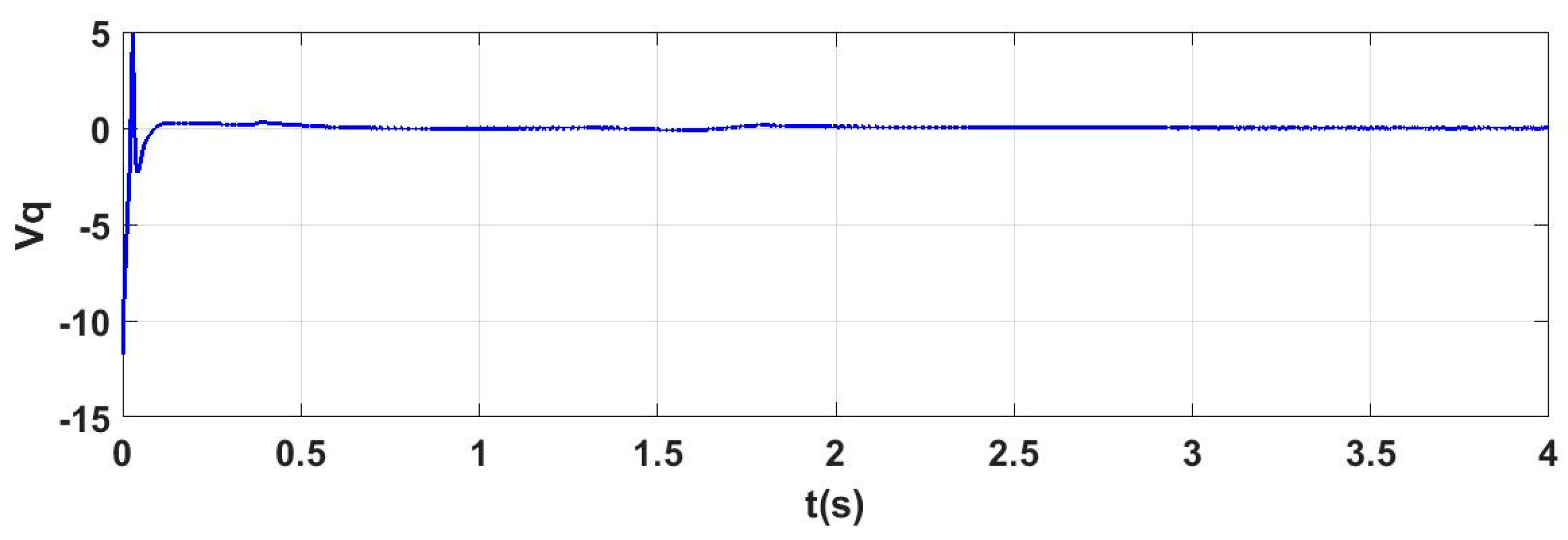
According to the Figure 9, the Voltage $v_q$ is equal to zero for all the time and this shows that the PLL is stable for optimal parameters of micro-grid and network (according to proposed stability criteria of PLL $u{p}_q=0$).

Now, the stability of PLL is examined for determined optimal values of micro-grid and network parameters by the second proposed Stability criterion in (27).

$${\phi }_P=\frac{\pi }{2}-{\mathit{tan}}^{-1}\left(-\frac{R_L+L_L·{\omega }_P+L_L·{\omega }_P·Z_{net}}{\left(Z_{net}.R_L\right)}\right)=3.11rad$$

(29)

$$I_{l2}<\frac{\left|u_{net}·K_{net}\right|}{\left|\mathit{sin}\left({\phi }_P\left({\omega }_P\right)\right)·K_P\right|}=\frac{230}{\left|10\mathit{sin}\left({\phi }_P\left({\omega }_P\right)\right)\right|}=60.3104$$

(30)

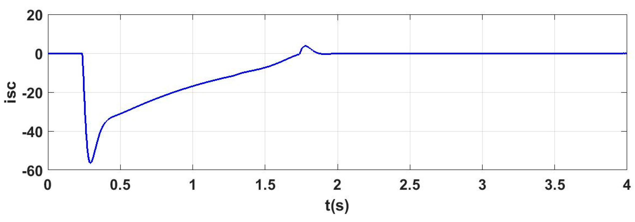
The Equation (30) implies that only the parameters that lead to the injection of the output current $I_{l2}$ less than 60.3144 amperes, ensure the PLL stability. According to the proposed criterion, it is clear that the PLL would be unstable for larger output current of inverter ($I_{l2}$), larger network impedances ($Z_{net}$) and larger reactive loads (${\phi }_P\left({\omega }_P\right)$). 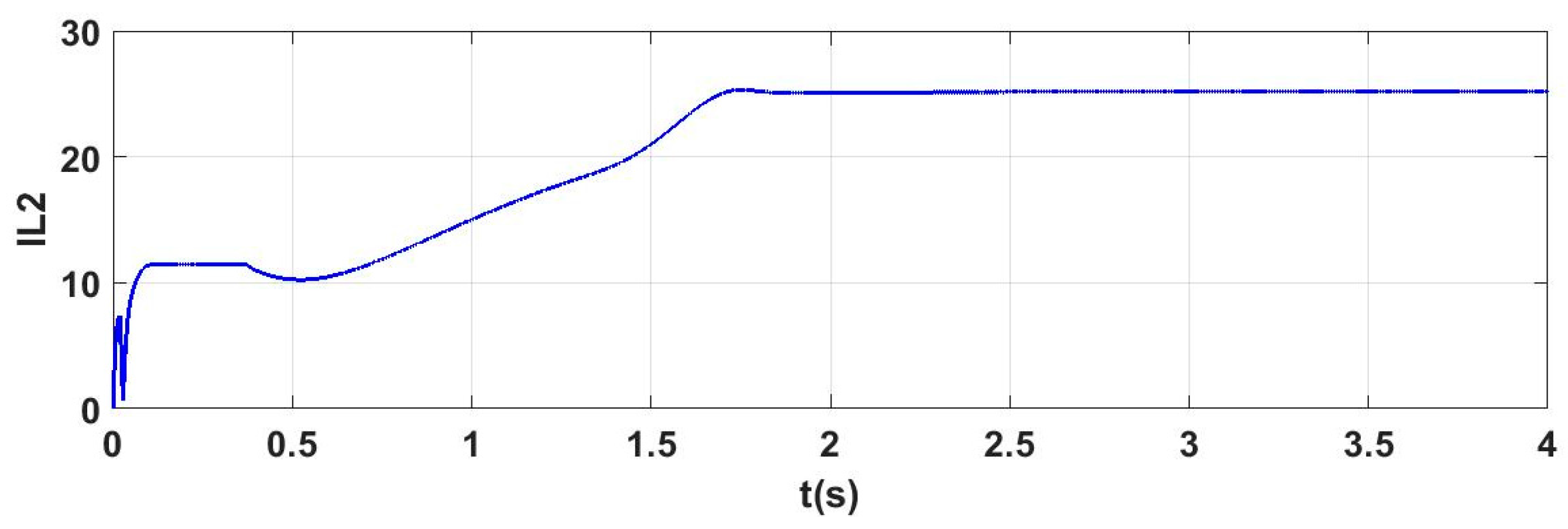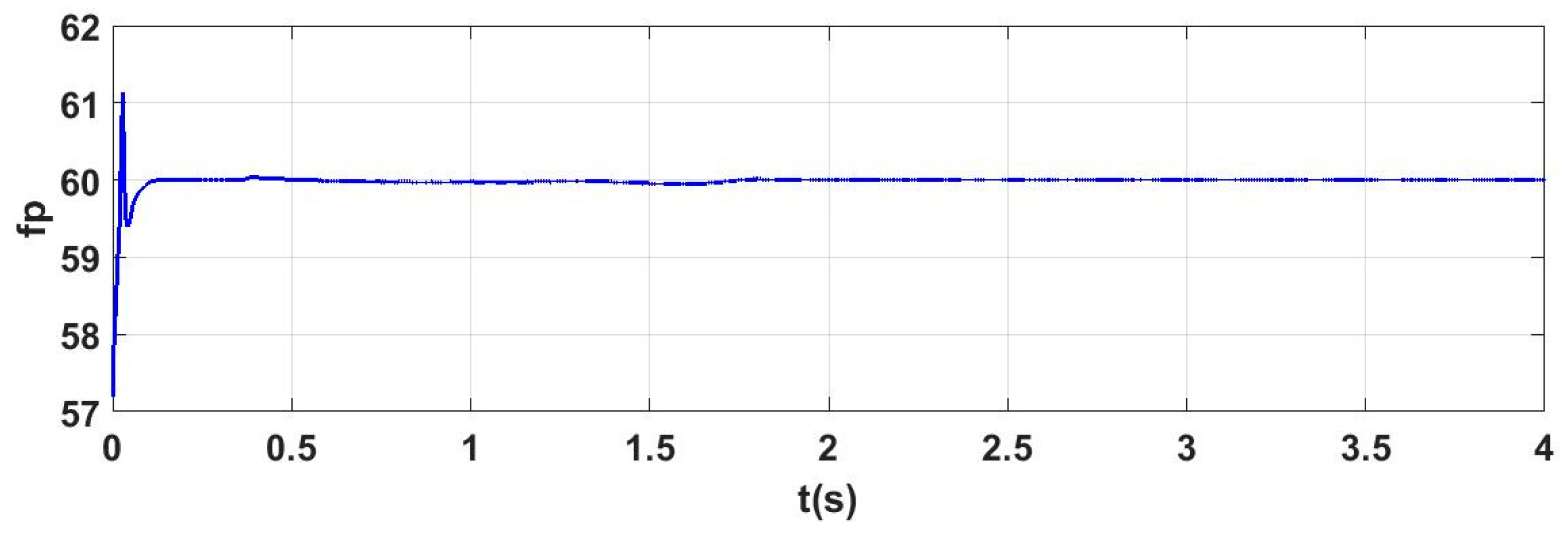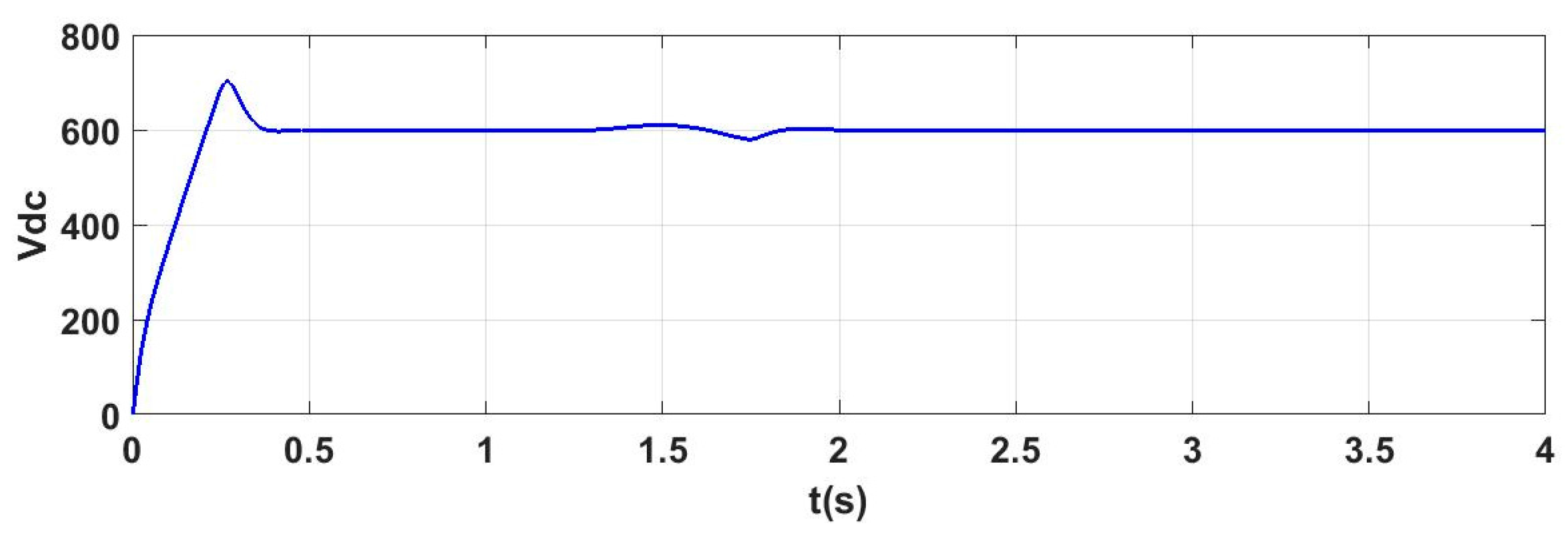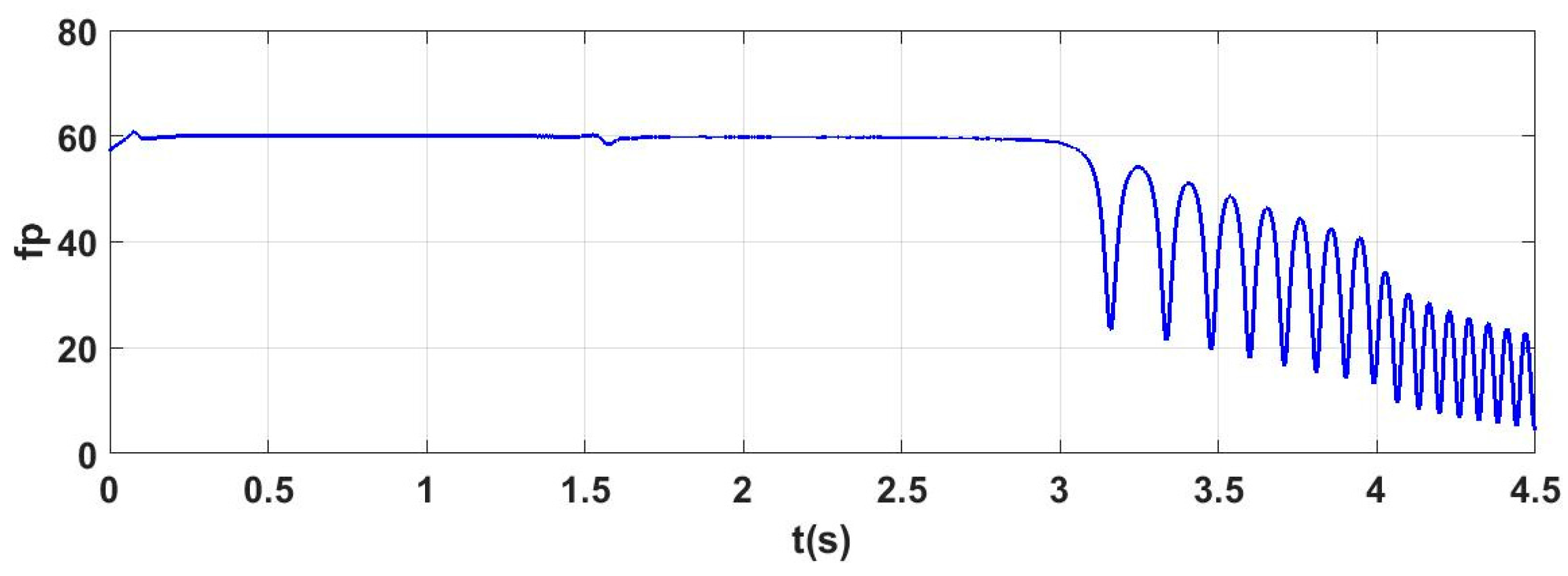The inverter output current $I_{l2}$ for optimal values of micro-grid and network parameters has simulated in Figure 10, it is clear that mentioned current has satisfied the New Stability criterion and therefore, the PLL is stable for optimal values of micro-grid and network parameters. As shown, PLL is stable according to the stability criteria for the optimal parameters of micro-grid and main network. Now for more reviews, the Output frequency of PLL, DC bus voltage and super-capacitor current has simulated in Figure 11, Figure 12 and Figure 13, respectively.

Figure 11, shows that the output frequency of the PLL is constant and equal to 60 Hz for all the times. This issue is evidence of the PLL stability. Figure 12 shows that for optimal values of micro-grid parameters, the DC bus voltage is stable and equal to 600 volts. That means, in addition to the PLL stability, the micro-grid is also stable.

As previously mentioned, toward increasing the battery life and also because the super-capacitor has a high response speed, sudden changes in power are compensated by a super-capacitor. This means that the high frequency error terms would be compensated by the super-capacitor, lower frequency terms by the battery and the rest would be compensated by means of the grid-interface converter. 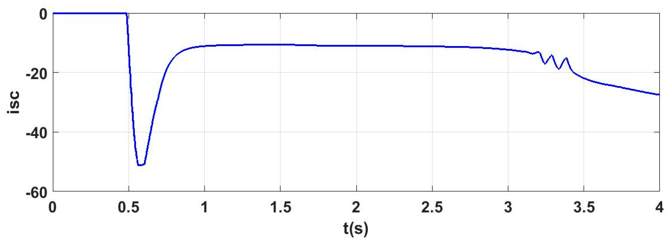As shown in Figure 13, the sudden power changes in the micro-grid has compensated by the super-capacitor and indicate that the optimal super-capacitor capacity has been correctly selected. It should be noted that, as stated in the previous section, in this study it has been assumed that the battery compensates a pre-specified current of about 10 amperes.

5. Assessing the Effect of Hybrid Storage System’s Parameters on PLL Stability

As mentioned above, the time constant of low-pass filter (τ) and the equivalent capacity of super-capacitor ($C_{sc}$) have great impact on the stability of PLL by more than 12 percent and it is in the third degree of importance (according to Table 3). According to the Result of variance analysis of signal to noise ratio (Table 3) and mean of signal to noise ratio (Figure 8) it is clear that by increasing the values of time constant and equivalent capacity of super-capacitor, the stability of PLL improves and, naturally, the stability of the PLL for the smaller values is imperiled.

5.1. Impact of the Time Constant of Low-Pass Filter (τ) on PLL Stability

In order to evaluate the effect of the time constant of low pass filter on the stability of PLL, it is assumed that the share of compensated current by battery has been pre-specified (about 10 amperes). In this case, the control system determines only the share of the super-capacitor and the grid-interface converter. As mentioned earlier, the share of each storage element and grid-interface converter is determined by adjusting the bandwidth of each filter. Since it is assumed that the share of compensated current by battery has been pre-specified, only a low-pass filter with transfer function $\frac{K}{1+s\tau }$ is used until the low-frequency terms of $i_{dis}$ is compensated by the grid-interface converter and the rest by the super-capacitor. In Figure 9, Figure 10, Figure 11, Figure 12 and Figure 13, the studied micro-grid was simulated for optimal micro-grid parameters. In fact, simulations were performed for the best parameters (best conditions). Now, to show the effect of each of the mentioned parameters, the studied micro-grid is simulated for the worst conditions. To investigating the effect of time constant of low-pass filter on PLL stability, the Simulations are performed for $\tau =0.5$ s. Since the time constant of low-pass filter has reduced from optimal value (10 s) to 0.5 s, so a larger share of the current is compensated by the converter. As shown in Figure 14, the Inverter output current $I_{l2}$ has exceeded from the value specified in Equation (30) and has led to the instability of the PLL. Since the Inverter output current $I_{l2}$ has exceeded from the stability limit, therefore, the $v_q$ also exceeds from zero value. This problem has shown in Figure 15 and confirms that both stability criteria have been violated and as a result, the PLL has been instable. According to the above mentioned, the output frequency of the PLL is also not stable, which is shown in Figure 16.

5.2. Impact of the Equivalent Capacity of Super-Capacitor ($C_{sc}$) on thePLL Stability

To investigating the effect of equivalent capacity of super-capacitor on PLL stability, the capacity value has considered the worst conditions ($C_{sc}=0.1\mathrm{F}$). The eigenvalues of studied micro-grid’s state matrix (in Equation (5)) for $C_{sc}=0.1\mathrm{F}$ are given in

Table 6. Eigenvalues of micro-grid’s state matrix for $C_{sc}=0.1$.

State Variables	Eigenvalues
${\tilde{i}}_b$	−54.11 + 294.64i
${\tilde{i}}_{sc}$	−127.54 − 74.01i
${\tilde{u}}_{dc}$	131.62 + 100.34i
${\tilde{i}}_{l1d}$	−24.73 +95.87i
${\tilde{i}}_{l1q}$	−24.73 − 95.87i
${\tilde{i}}_{l2d}$	15.06 + 95.87i
${\tilde{i}}_{l2q}$	−9.05
${\tilde{i}}_{LLd}$	−15.13 − 10.15i
${\tilde{i}}_{LLq}$	−15.13 + 10.15i
${\tilde{u}}_{cfild}$	−12.76 − 93.98i
${\tilde{u}}_{sc}$	−12.76 + 93.98i
${\tilde{u}}_{pd}$	−24.23
${\tilde{u}}_{pq}$	6.53
$\tilde{C}$	9.04 − 18.42i
${\tilde{\theta }}_P$	9.04 + 18.42i

.

The indicated Eigenvalues in Table 6 show that the studied micro-grid and also the PLL of grid-interface converter are instable for $C_{sc}=0.1\mathrm{F}$.

Also, for confirmation of the obtained results from the analysis of the Eigenvalues and the proposed stability criteria of PLL, the studied micro-grids simulated for $C_{sc}=0.1\mathrm{F}$.

In this case, given that the equivalent capacity of the super-capacitor has decreased from its optimal value (3 F) to 0.1 F and also because the time constant is 10 s, a significant current passes from the super-capacitor. Therefore, the super-capacitor voltage increases substantially, which makes the PLL instable.

The resulting simulations in Figure 17, Figure 18, Figure 19 and Figure 20 confirms the obtained results from the analysis of the Eigenvalues and the proposed stability criteria of PLL.

6. Conclusions

In this paper, two new stability analysis criteria for the PLL affected by parameters of micro-grid and hybrid storage system are presented. The optimal values of micro-grid and hybrid storage system parameters to improve the stability of PLL and thereby the stability of the network-side converter was determined. The dynamic model of micro-grid was simulated in MATLAB software area. Taguchi approach was employed in order to determine the optimum levels of the micro-grid and hybrid storage system parameters. Moreover, variance analysis was used to prove the meaningful effect of these parameters on the output. Results of statistical analysis showed that some micro-grid and hybrid storage system parameters, which have been evaluated in this study, have significant effects on the PLL stability and thus the grid (network)—side converter stability. Finally, the PLL stability affected by hybrid storage system parameters was investigated. The simulation results and eigenvalues analysis confirmed the theoretical analysis and proposed criteria.