Topology-Based Estimation of Missing Smart Meter Readings

Abstract

Smart meters often fail to measure or transmit the data they record when measuring energy consumption, known as meter readings, owing to faulty measuring equipment or unreliable communication modules. Existing studies do not address successive and non-periodical missing meter readings. This paper proposes a method whereby missing readings observed at a node are estimated by using circuit theory principles that leverage the voltage and current data from adjacent nodes. A case study is used to demonstrate the ability of the proposed method to successfully estimate the missing readings over an entire day during which outages and unpredictable perturbations occurred.

1. Introduction

Advanced metering infrastructures (AMI) in distribution networks provide grid operators with information that can be utilized for various operations such as state estimation, voltage control, aggregation of power consumption, and fault detection. A crucial benefit of AMI is real-time demand response (DR) based on real-time retail pricing. Real-time DR realizes peak savings [1,2,3], maximizes the benefits of consumers or retailers [4,5,6,7], and reduces line losses [5]. The prerequisite conditions for implementing real-time pricing are accuracy and continuity as well as the absence of delays in measurements at each consumer site. However, meter readings are often incomplete because of missing readings as the meter metrology and communication module regularly malfunction. In addition, there are other causes that can lower the accuracy of measurements such as significant time desynchronization, incorrect selection of current and power transformers, and faulty installation processes [6]. Even though the percentage of missing readings in typical scenarios seems to be small, the actual number of missing readings ultimately proves to be very high. A recent study [7] found the number of installed smart meters in the United States to have reached 45.8 million, which represents a penetration level of approximately 30%. Other researchers [8,9,10,11] established that AMI systems fail to record between 2.7% and 9.4% of meter readings in a given year.

Approaches to compensate for these missing readings included the interpolation of the missing readings by taking an average of adjacent correct readings [12,13]. The results from this approach hardly convinced customers to pay their bills because the mean value is not a good representation of the actual usage. In addition, the difference between the actual and interpolated readings increases as the number of missing readings increases. Short-term load forecasting (STLF) is one of the alternative methods to estimate missing readings. STLF for aggregated energy consumption at a substation or an MV feeder was proposed [14,15,16,17,18]. The work in [14] proposes a data-driven probabilistic net load forecasting method designed to handle a high penetration of behind-the-meter PV. Among these the solution with the best performance is described in [18], this work proposes a day-ahead forecasting with small errors varying between 0.753% and 2.37%. STLF is also applied to a smart meter in a secondary network in [19,20,21], however, this method was found to drastically decrease the reliability of the estimation. In [19], statistical forecasting for secondary networks is shown to require sufficient information such as the wind-chill temperature, humidity index (humidex), day load patterns and historical loads. The error of estimation was found to be between 37% and 105%. Several methods regarding day-ahead forecasting for smart meters were compared in [20], in these works the prediction for each consumer (smart meter) was performed with an error of at least 20%. The work in [21], details a 30 min ahead prediction performed based on regression tree model. Even though this work uses much more data parameters, such as room temperature and feature of the AC air conditioner, the prediction achieves an accuracy of about 21.3%. State estimation methods are also proposed in [22,23]. In [22], state estimation methods based on historical measured data is proposed with uncertainty of the network topology information. In [23], the state variables such as voltage and angle is estimated by neural network. These state estimation methods utilized angle which must be measured by phasor measurement unit (PMU). In the lowest voltage network where users connect, such sophisticated devices are not available. As such to compensate for missing meter readings, state estimation is not useful.

Other approaches to estimate missing readings, including the generation of pseudo-measurements to interpolate missing readings [9], also the utilization of data cleansing methods based on regression analyses to estimate missing readings is proposed by [24,25]. However, the works by [24,25] does not discuss the accuracy of estimation of the proposed methods for meter readings. The latter study [25] involved the intentional production of simulated missing readings by intermittently removing 30% of the meter readings from the complete dataset. In view of this the numerical forecast cannot guarantee an accurate prediction in the case of missing readings resulting from long-term measurements such as those acquired during the course of a day. Adding to this, the accuracy decreases in the case of load patterns that containing outages or accidental demand perturbations. For each customer, based on regression model, it is difficult for the estimation of missing readings with high resolution. This is because the trend of each customer’s energy usage may easily change owing to user’s unpredictable behavior such as going on a trip, relocation, purchasing new appliances.

A review of existing work revealed the following general types of weaknesses in the methods proposed to date: (1) average methods, such as those in which the average of adjacent correct readings is taken, do not represent actual consumption; (2) existing load forecasting algorithms cannot realize the necessary accuracy required by a smart meter; (3) data cleansing methods based on regression models are useful in the case of regular load patterns; however, they cannot guarantee accuracy in the case of accidental or irregular load variation.

To overcome the above problems, we propose an analytical method to estimate missing readings with well-grounded circuit theory principles. The proposed method utilizes voltage and current values from adjacent nodes that remained intact during the missing period. These data are used to estimate the current, voltage, and power factor of the missing meter node, and subsequently, to infer the power consumption of the node. Missing current and voltage are represented as variables of nonlinear simultaneous equations. The missing data are obtained as solutions of the equations that can be solved by numerical methods. Because the numerical methods cannot guarantee an exact solution, it is necessary to verify the accuracy of the estimation. One advantage the proposed method has is that it does not rely on past readings or any supplementary data, i.e., past load profile or weather-related data. Therefore, it does not matter if missing readings are out of periodicity for a past pattern. Another advantage of the proposed method is that it can manage long-term missing readings and outliers in missing readings. Because the proposed method is not based on the trend of the past energy usages, as long as the voltage and current at neighboring nodes of the missing meter node is intact, the missing readings can be estimated regardless of the duration of the missing period. Moreover, the proposed method is practical because it does not utilize phasor difference information between readings of different smart meters. Smart meters distributed in the actual field cannot synchronize with each other within the order of milliseconds; therefore, phasor difference information is not considered.

The remainder of this paper is organized as follows: Section 2 describes the premise, model, and formulation of the proposed method. Section 3 presents the verification of the estimation accuracy for successive missing readings containing outliers in a given day. The simulation results show that the proposed method reliably estimates not only the periodic values but also the outliers. Section 4 discusses the simulation result with some practical assumptions. Finally, the proposed work is summarized and concluded in Section 5.

2. Model and Formulation

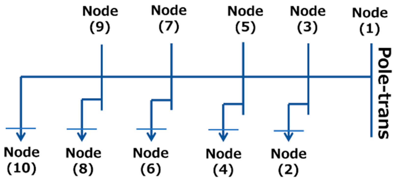
2.1. Model and Premises

Figure 1 shows an example of load variation in a specific network in which meter readings recorded between 1 p.m. and 1:15 p.m. are missing. Node(2) in Figure 1 is the missing meter node that fails to transfer its meter readings to the servers. This study considers a case in which only one node in the network failed to transmit its data during a specific interval. The neighbors of the missing meter node, whose meter readings are correctly received at the servers during the same period, are Node(1) and Node(3). In general, to reduce the amount of data transmitted, smart meters transfer only their total energy consumption, as indicated by the grayed-out area in Figure 1. The received meter readings related to each customer’s information are then stored in the database on the server. The procedure for detecting and estimating missing readings is as follows:

(1)

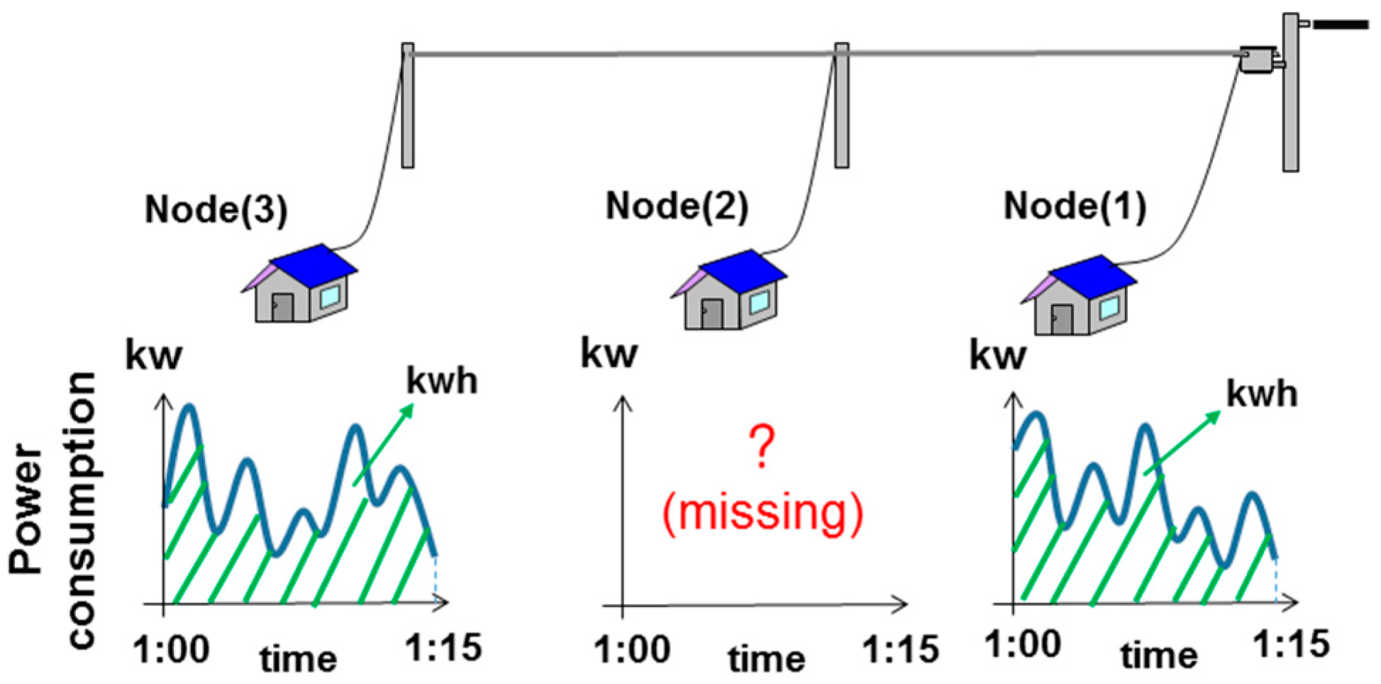
Detection: Servers receive meter readings every 15 min. If the servers do not receive a reading, the servers log the details of the missing meter node that fails to transfer the reading.

(2)

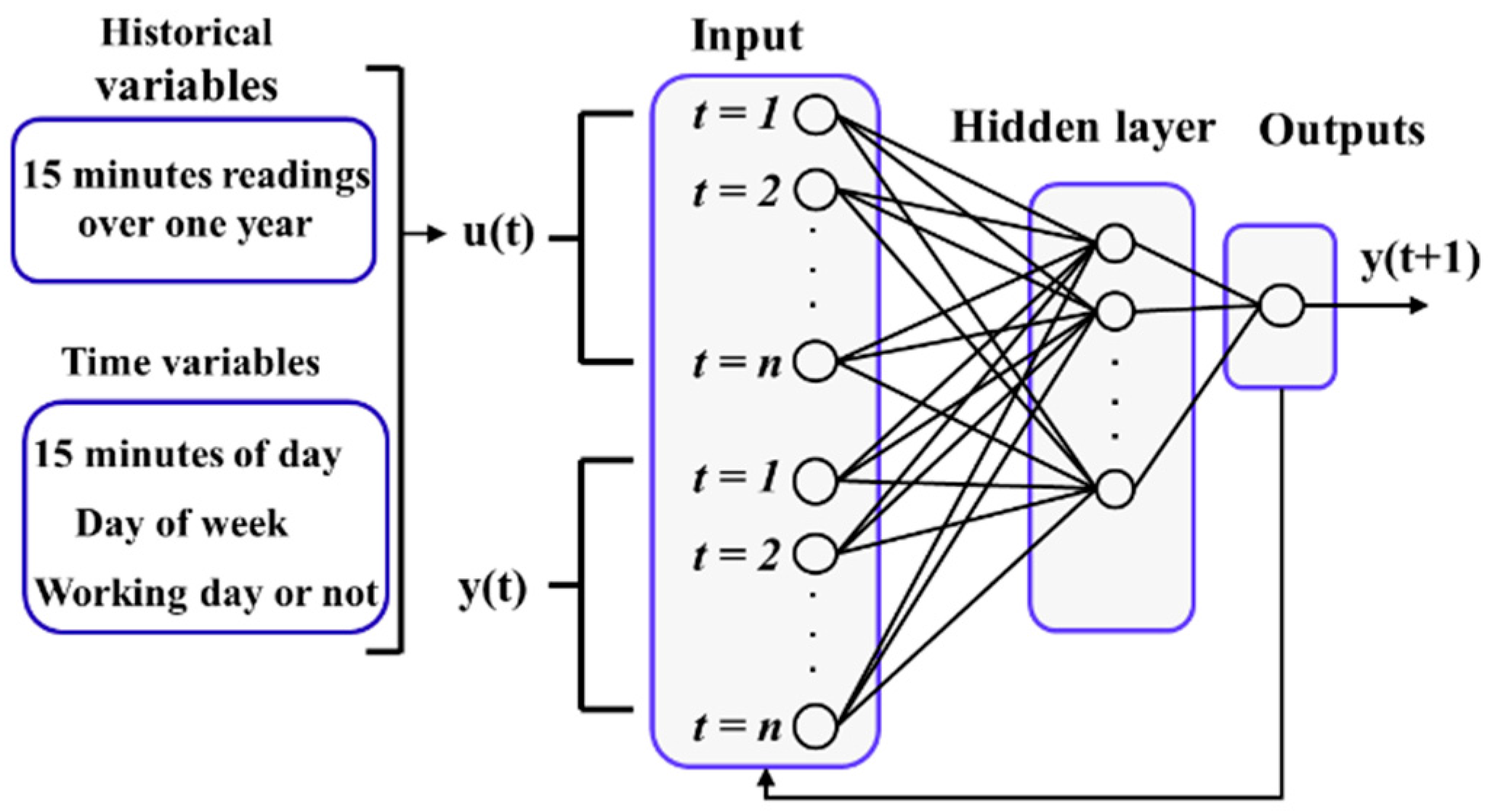
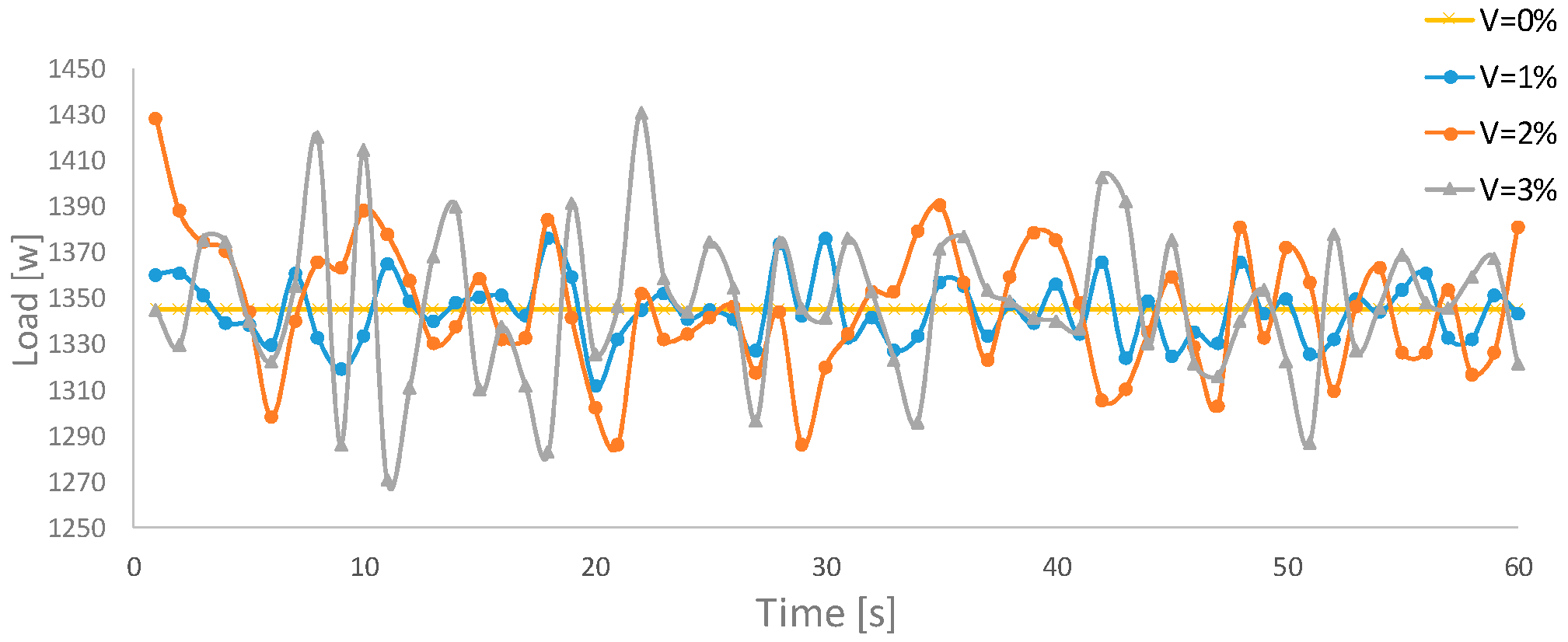
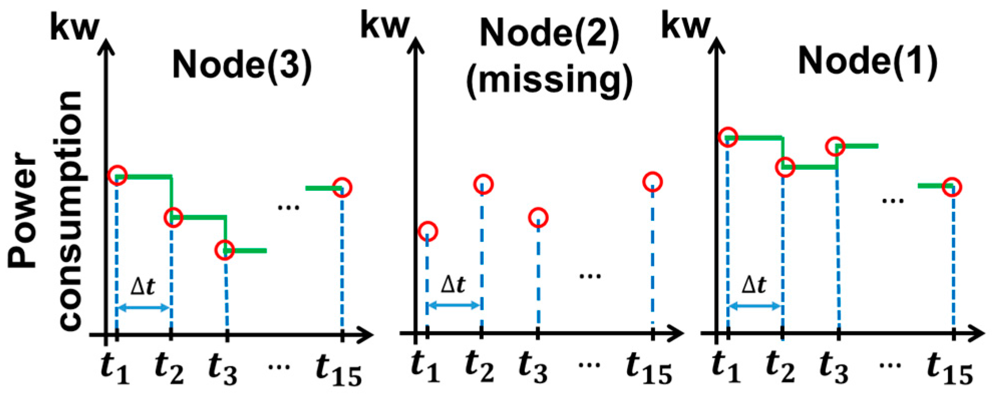
Operation: Once the servers detect the missing meter node, the servers request the neighboring nodes to send voltage, current, and power factor data for instances during the period coinciding with the missing reading. These data from the neighbors are used to estimate the missing reading. The resolution of the time instance data is assumed to be 1 min. All smart meters store time instance data for the immediate past 15 min.

(3)

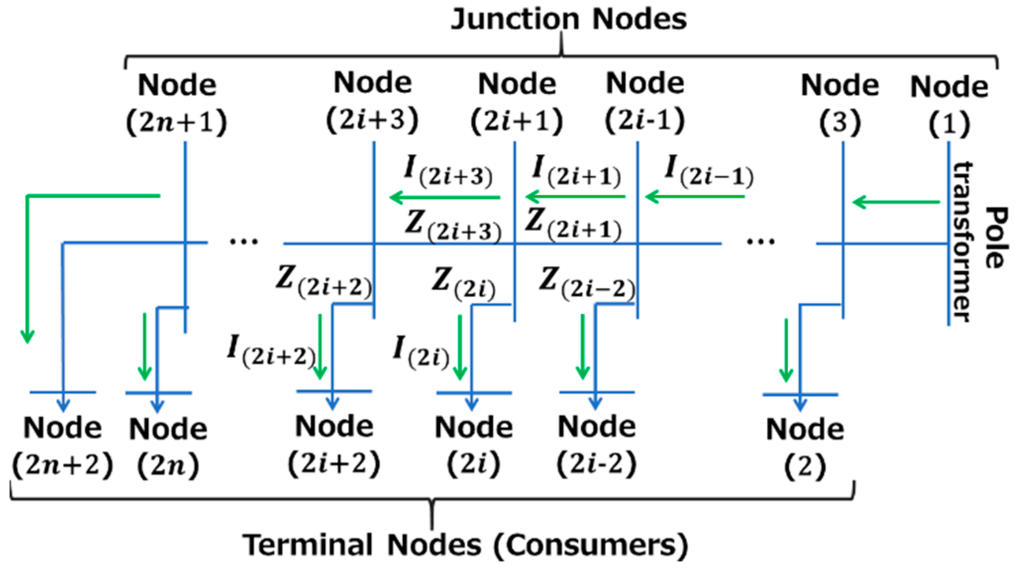
Estimation: The span of 15 min is divided into even periods of ∆t as shown in Figure 2. In this study, ∆t is assumed to be one minute and active power consumption is assumed to be fixed during ∆t. The power consumption for the time instances indicated with circles in Figure 2 are defined along with $t_1$, $t_2$, $t_3,$ …, $t_{15}$. The missing load variation at Node(2) is estimated according to the following procedure. Based on the measured values for current, voltage, and energy consumption at Node(1) and Node(3) at time $t_1$, the values for the missing voltage and current data at Node(2) at time $t_1$ are calculated by utilizing circuit theory principles as shown in Section 3. The active power instances at $t_1$ followed by $t_2$, $t_3$, …, $t_{15}$ are also estimated in the same way as at $t_1$. Estimation of the 15 active power instances at Node(2) enables the energy consumption at the instances between $t_1$ and $t_{15}$ to be obtained for Node(2).

The smart meters distributed in each region have different specification and work under various policies. In some countries, the regulatory framework does not allow the distribution system operator to collect and use current and voltage parameters. In this paper, we discuss estimation of missing meter readings from the view point of technique. To implement the proposed method on a real-time grid network, system operator needs to collecting current and voltage parameters from each customer. The process of collecting such parameters should take into consideration privacy and security while conforming to set policy.

The generalized network model of the proposed method, which is derived from that in Figure 1, is indicated in Figure 3. The terminal nodes (T-nodes) are the consuming nodes. The junction nodes (J-nodes) are common nodes and do not have energy sources. The number of consumers is expressed as n, which is assumed to be larger than three. The flow of current is indicated by the direction of the arrows. It is noted that the J-nodes are not equipped with smart meters, and therefore, the current injected into this distribution network cannot be measured.

In this study, the network topology and the order of the T-nodes are assumed to be given. Circuit parameters such as the impedance and topology are known to be ambiguous, especially in the secondary distribution network. However, collecting and updating the impedance and topology manually is not feasible in terms of the cost; thus, it is necessary to estimate both of these parameters automatically without human intervention. The impedance can also be estimated based on the meter readings [26]. Regarding the topology, secondary distribution networks are known to be mainly composed of a radial network [27,28]. Therefore, the proposed method focuses on the radial structure. AMI systems actually may be able to approximate the time synchronization to within a few seconds in terms of specification. Because different meters are asynchronous within a few seconds or less than one minute, the phasor difference between measurements recorded by different smart meters is not available. Therefore, the proposed method utilizes only the root mean square (RMS) current, voltage, and power factor at each node. The proposed method can accept the time difference between smart meters without changing the RMS values. In this work, the RMS values at each node are assumed not to change during a period of one minute.

2.2. Formulation

This section presents the construction of nonlinear simultaneous equations of which the unknown variables are the missing current, voltage, and power factor. Once the equations are composed, the missing data are obtained as solutions for these equations. The missing readings at the missing node are represented using the RMS voltage and current measured at both adjacent nodes. The end T-node is Node(2n + 2) in Figure 3, whereas the initial T-node is Node(2). All T-nodes other than the end and initial T-node are denoted middle T-nodes. In case the node with missing readings is located at the end of a network, the measured RMS voltage and current at one adjacent node are required. Similarly, in case the node with missing readings is the initial node, the RMS voltage at the pole-transformer is required. Because the voltage of the pole-transformer is not actually stable, the extent to which the voltage fluctuation at the pole-transformer affects the estimation of the missing readings is evaluated in Section 4.

The following formulation relates to the case in which the missing node is located at the end of the network. The formulation for the cases in which the other nodes have missing readings is presented in the Appendix A. In the following equations, variables that cannot be directly measured with a smart meter are indicated with “^”. For example, the voltage at Node(2i − 1) is unmeasurable because Node(2i − 1) does not have a smart meter. Therefore, the voltage of Node(2i − 1) is expressed with “^” in the term ${\widehat{V}}_{(2i-1)}$. If the phase reference for all variables is the voltage at Node(2i + 2), the voltage at Node(2i − 2) is expressed as ${\widehat{V}}_{(2i-2)}$ even though Node(2i − 2) has a smart meter, because the phase difference between these two nodes is unmeasurable. The RMS voltage at Node(2i − 2) is expressed without “^” as $|V_{(2i-2)}|$, because at all T-nodes, the RMS voltage values excluding the phase difference information are measurable. The voltage and current at a missing meter node are also expressed with “^”. To infer the validation curve of active power along with the missing readings during a specific period at a missing meter node, two cost functions are formulated. These cost functions relate to the voltage at Node(2n + 1) and Node(2n − 1), respectively. The voltage at Node(2n + 1) is expressed based on the following measurable information at Node(2n + 2):

$${\widehat{V}}_{(2n+1)}=V_{(2n+2)}+I_{(2n+2)}{Z}_{(2n+2)}$$

(1)

The phase reference is considered $V_{(2n+2)}$ in Equation (1). The voltage at Node(2n + 1) can also be expressed based on the unknown information at the missing meter node Node(2n) as follows:

$${\widehat{V}}_{(2n+1)}={\widehat{V}}_{(2n)}+{\widehat{I}}_{(2n)}{Z}_{(2n)}$$

(2)

The phase reference in (2) is also considered $V_{(2n+2)}$. The first cost function is derived from Equations (1) and (2), which should be equal.

$$f_1({\widehat{V}}_{(2n)},{\widehat{I}}_{(2n)})\equiv V_{(2n+2)}+I_{(2n+2)}{Z}_{(2n+2)}-{\widehat{V}}_{(2n)}-{\widehat{I}}_{(2n)}{Z}_{(2n)}=0$$

(3)

The other cost function is formulated regarding the voltage at Node(2n − 1). The voltage at Node(2n − 1) is expressed based on the measurable information at Node(2n − 2) as follows:

$${\widehat{V}}_{(2n-1)}=V_{(2n-2)}+I_{(2n-2)}{Z}_{(2n-2)}$$

(4)

The phase reference in Equation (4) is $V_{(2n-2)}$. The voltage at Node(2n − 1) can also be expressed based on the information at Node(2n + 1) as follows:

$${\widehat{V}}_{(2n-1)}={\widehat{V}}_{(2n+1)}+(I_{(2n+2)}+{\widehat{I}}_{(2n)})Z_{(2n+1)}$$

(5)

The phase reference in Equation (5) is $V_{(2n+2)}$, and in this equation, ${\widehat{V}}_{(2n+1)}$ is already expressed by the measurable values as Equation (1). From Equations (4) and (5), the second cost function is obtained as follows:

$$f_2({\widehat{V}}_{(2n)},{\widehat{I}}_{(2n)})\equiv |V_{(2n-2)}+I_{(2n-2)}{Z}_{(2n-2)}|-|{\widehat{V}}_{(2n+1)}+(I_{(2n+2)}+{\widehat{I}}_{(2n)})Z_{(2n+1)}|=0$$

(6)

In Equation (6), only the absolute values of the first and second terms on the right-hand side are taken to avoid taking the phase difference into consideration. The phase reference of ${\widehat{V}}_{(2n-1)}$ is expressed in Equation (4) in terms of $V_{(2n-2)}$. On the other hand, the phase reference of ${\widehat{V}}_{(2n-1)}$ is expressed in Equation (5) in terms of $V_{(2n+2)}$. To compare two voltages with different phase references, it is necessary to take the absolute value. Now, Equations (3) and (6) are the nonlinear simultaneous equations with the unknown variables of ${\widehat{V}}_{(2n)}$ and ${\widehat{I}}_{(2n)}$, which represent the missing voltage and current data. Our primary goal is to find the values of these unknown parameters that satisfy both equations. Because the equations are nonlinear, it is generally not possible to find the solution analytically. Instead, a numerical approach can be utilized to seek solutions. We incorporate an optimization scheme to seek the unknown variables with the following objective function.

$$Min(\Vert f_1({\widehat{V}}_{(2n)},{\widehat{I}}_{(2n)}),f_2{({\widehat{V}}_{(2i)},{\widehat{I}}_{(2i)})\Vert }_{\infty })$$

(7)

Note that other types of objective functions such as the Euclidian norm can be utilized as well to find solutions for the equations. In this work, we chose the infinity norm experimentally, as it showed the best performance with the iterative optimization method known as particle swarm optimization. This method was employed for the case study in Section 3. The actual power factor measured at households in South Korea, which was provided by the electricity supplier KEPCO, generally ranges from 0.97 to 1.00. Therefore, the constraint regarding the power factor at each T-node is adopted as follows:

$$0.97<\frac{Real({\widehat{S}}_{(2n)})}{\sqrt{Real{({\widehat{S}}_{(2n)})}^2+Imag{({\widehat{S}}_{(2n)})}^2}}<1.00$$

(8)

where

$${\widehat{S}}_{(2n)}={\widehat{V}}_{(2n)}{\widehat{I}}_{(2n)}^{*}$$

(9)

where ${\widehat{I}}_{(2n)}^{*}$ signifies the conjugate of ${\widehat{I}}_{(2n)}$.

Regarding the T-nodes in the middle, and the initial T-node, the objective functions are analogically formulated, and is explained in the Appendix A.

3. Case Study

This section, which presents the case study, is composed of two parts: Section 3.1 and Section 3.2. In Section 3.1, a simulation is described that was performed to validate the accuracy of the proposed method. The case study was designed to prove that the proposed method can estimate missing readings when successive meter readings are missing from data recorded during an entire day and when the load variation (missing readings) contains unpredictable phenomena such as demand responses and outages. The simulation result of the proposed method is compared with other major methods: a neural network (NN)-based method and the average method. Subsequently, various load patterns were adopted as missing meter readings, as discussed in the case study in Section 3.2. The objective of the latter case study was to determine whether the proposed method would be effective regardless of the type of load patterns observed in the actual measurement data.

In both of the case studies in Section 3.1 and Section 3.2, when the initial node has the missing readings, the RMS voltage of the pole-transformer is assumed to be a known parameter based on its specifications or measurement sensors. Other than for the initial node, this assumption is unnecessary. Additional practical cases, such as the voltage fluctuations at the pole-transformer in the specified range, are discussed in Section 4.

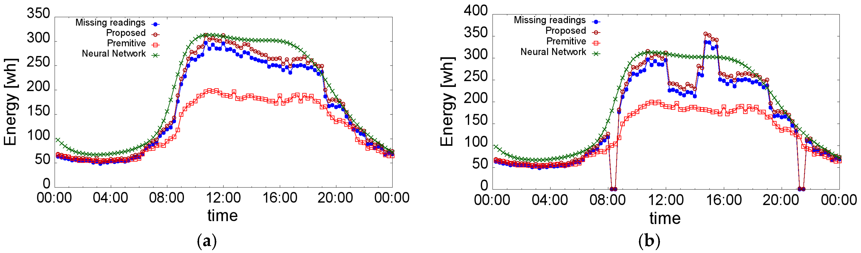
3.1. Performance Validation Compared with Other Methods

As shown in Figure 4, the model in this case study has five consumers in a secondary distribution network. Figure 5a shows data that was actually generated by and measured in a household in Korea on 2 January 2014 for the duration of the entire day, and which we consider for determining the missing readings in our case study. The missing load curve in Figure 5b contains outliers that are artificially produced from the load curve in Figure 5a. In Figure 5b, it is assumed that outages are observed from 8:00 to 8:30 and from 21:00 to 21:30. Demand response is also assumed from 12:00 to 14:00 and from 14:30 to 15:30. The proposed method is compared with two popular methods: the NN-based method presented in [15,20] and the average method adapted in [12,13].

• Proposed method

The proposed method is based on circuit theory as explained in Section 3; therefore, the position of the missing meter node can affect the accuracy of estimation. Five cases, in which the missing meter node is located at Node(2), Node(4), Node(6), Node(8), and Node(10), respectively, were examined to validate the accuracy of the proposed method in terms of the varying location of the missing meter node.

• NN-based regression method

A design based on one-hidden-layer multilayer perceptrons (MLPs), which are known as universal approximators [29], was adapted as the NN-based method. Therefore, in this case study, one-hidden-layer MLPs are adapted as in [15]. The problem presented by building the NN model is to select the input variables. Existing studies regarding load forecasting at the MV or substation level in [15,17,19] could be referenced to decide the relevant variables for this case study. These previous studies used past load data (30 min resolution), temperature data, and calendar variables [15], past load data, day of the week, and forecasted weather [19], and hourly past load data, past daily temperature, daily forecasted temperature, and day of the week [17], respectively. Considering these studies, the following variables were chosen as input values for this case study: past load data for a year (15 min resolution), 15 min section of the day (from 1 to 96), day of the week (from 1 to 7), working day or not (0 or 1). Weather-related data such as the humidity or temperature is not available for these load data; therefore, this case study did not consider weather factors. The structure of the NN model is illustrated by way of a diagram in Figure 6. Meter readings (15-min interval data in kWh) recorded during the entire year of 2013 were utilized as historical variables to train the learner. The number of neurons in the hidden layer also needed to be adjusted. A suitable number of hidden neurons were determined by estimating the usual load curve shown in Figure 7a by varying the number of hidden neurons. This number was varied from one to ten because typically a count smaller than ten hidden neurons is common for smart meter level forecasting [15,20]. In the case study using this NN-based model, a structure containing six neurons was adapted to realize the best performance and the delay was set as two.

• Average method

The average method was implemented by using the average data from the day preceding and the day following the missing day. In this case study, the missing day was 2 January 2014. The average estimation load curve was produced by taking the average data for 1 January and 3 January 2014. In this year, 1 January was a holiday in Korea, but 2 and 3 January were weekdays. Therefore, the result of the average method was considered as one of the worst cases.

Figure 7a,b indicate the load variations without and with outliers and their estimation accuracy, respectively. Figure 7b shows the results of the estimation based on the proposed method, the average method, and the NN-based method. In this study, the mean average percentage error (MAPE) and root-mean-square error (RMSE) are taken as evaluation criteria. A lower value of these criteria represent that the method contains a smaller error and is, hence, more accurate. Figure 8 summarizes the values obtained for MAPE and RMSE between the missing and estimated meter readings for the average, the NN-based, and the proposed methods, respectively. In Figure 8, the average and NN-based methods do not rely on the location of the missing meter node; therefore, the result is shown as one graph. On the other hand, regarding the proposed method, the five cases for each location of the missing meter node are shown. According to Figure 7a,b, the average method contains considerable errors that would not be acceptable in practice. The RMSE obtained for the NN-based method, shown in Figure 8, is smaller than that of the average method because the curve produced by the NN-based method approximately reproduces curve representing the missing readings between 9:00 and 19:00 as shown in Figure 7b. As shown in Figure 8a,b, the proposed method is superior to the NN-based and average methods in terms of both the MAPE and RMSE in both load variation cases. Even though the load variation contains outliers, the proposed method realizes almost the same accuracy as the situation with load variation without outliers. This is because the proposed method accurately follows the outages and perturbations as shown in Figure 7. Further, Figure 8 indicates the extent to which the location of the missing meter node affects the accuracy of estimation of the proposed method; however, the error rate of the proposed method in determining the varying location of a missing meter node would be acceptable compared to the accuracy of the average and NN-based methods.

The results in

Table 1. Comparison of accuracy for the estimation of missing smart meter readings.

	Proposed Method										Load Forecasting		Data Cleansing
	Node(2)		Node(4)		Node(6)		Node(8)		Node(10)
	(a)	(b)	(a)	(b)	(a)	(b)	(a)	(b)	(a)	(b)	[19]	[20]	[25]
MAPE (%)	6.8	6.7	7.1	7.2	6.7	6.6	3.9	4.0	5.2	5.0	37–105	20–30	6–8

cannot be exactly compared with each other because every method uses a different data set and prerequisites. The results in Table 1 show that the proposed method demonstrates the same or higher accuracy than the existing methods even though the missing readings are successive and contain outliers.

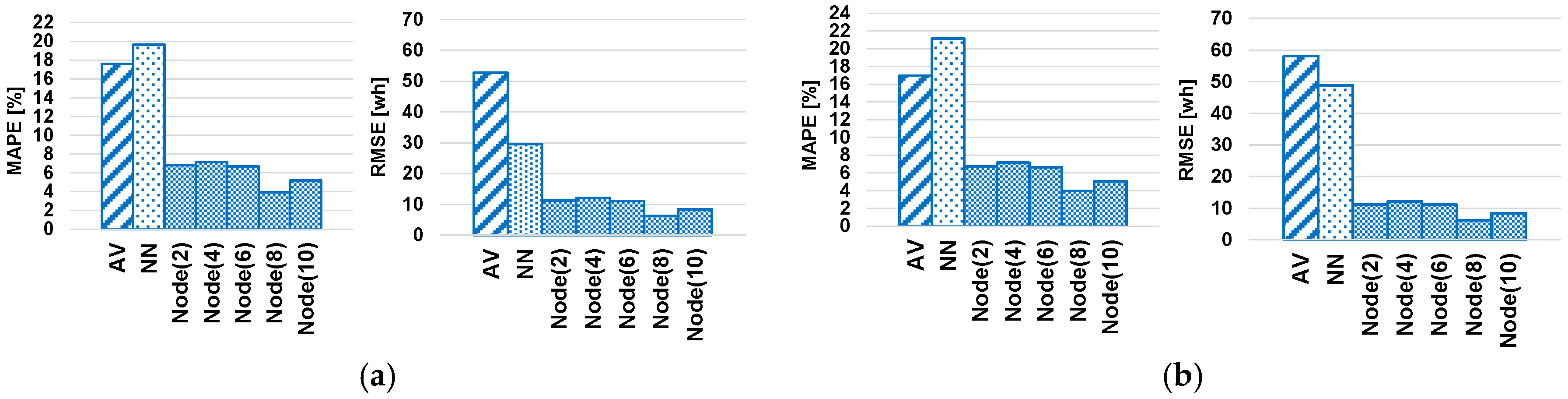
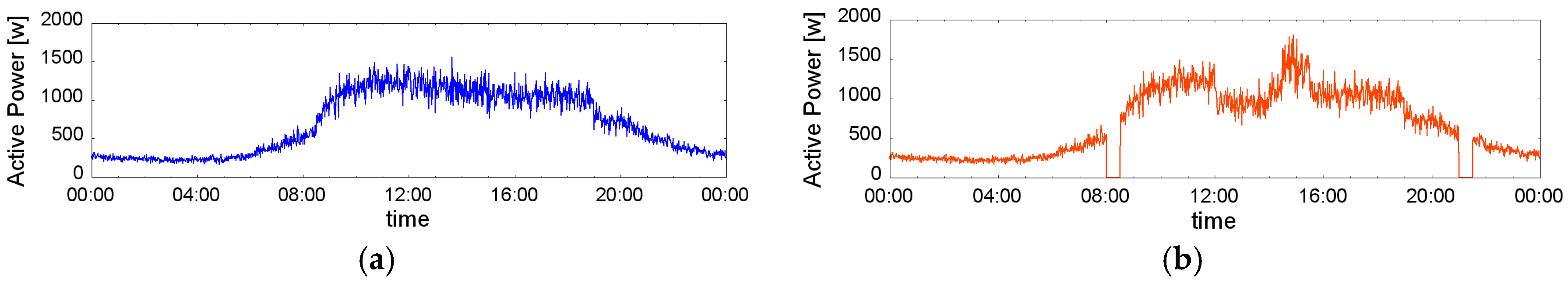
3.2. Performance Validation with Various Load Patterns

This section describes the validation of the proposed method using classified load data from an entire year, as shown in Figure 9, to confirm the effectiveness of the proposed method with various load patterns. Similar daily load patterns in the data set are classified into groups as shown in Figure 10. Then, one load pattern is selected from each group and these groups are shown in Figure 11. The selected patterns as representative of each group are taken to be missing readings to be estimated by the proposed method. The effect of these load patterns on the accuracy of estimation is validated.

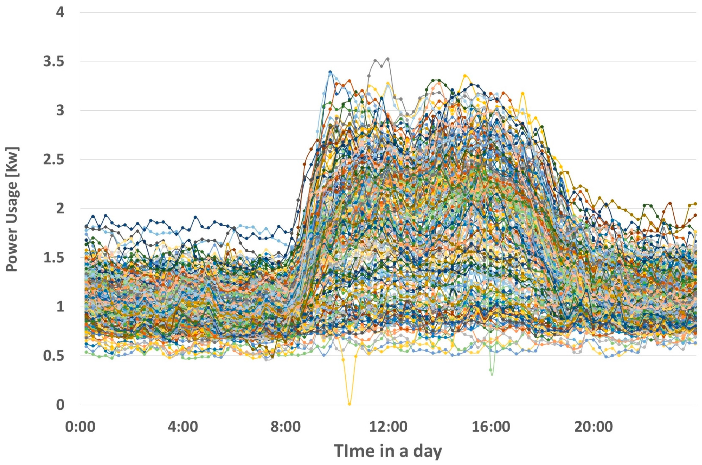
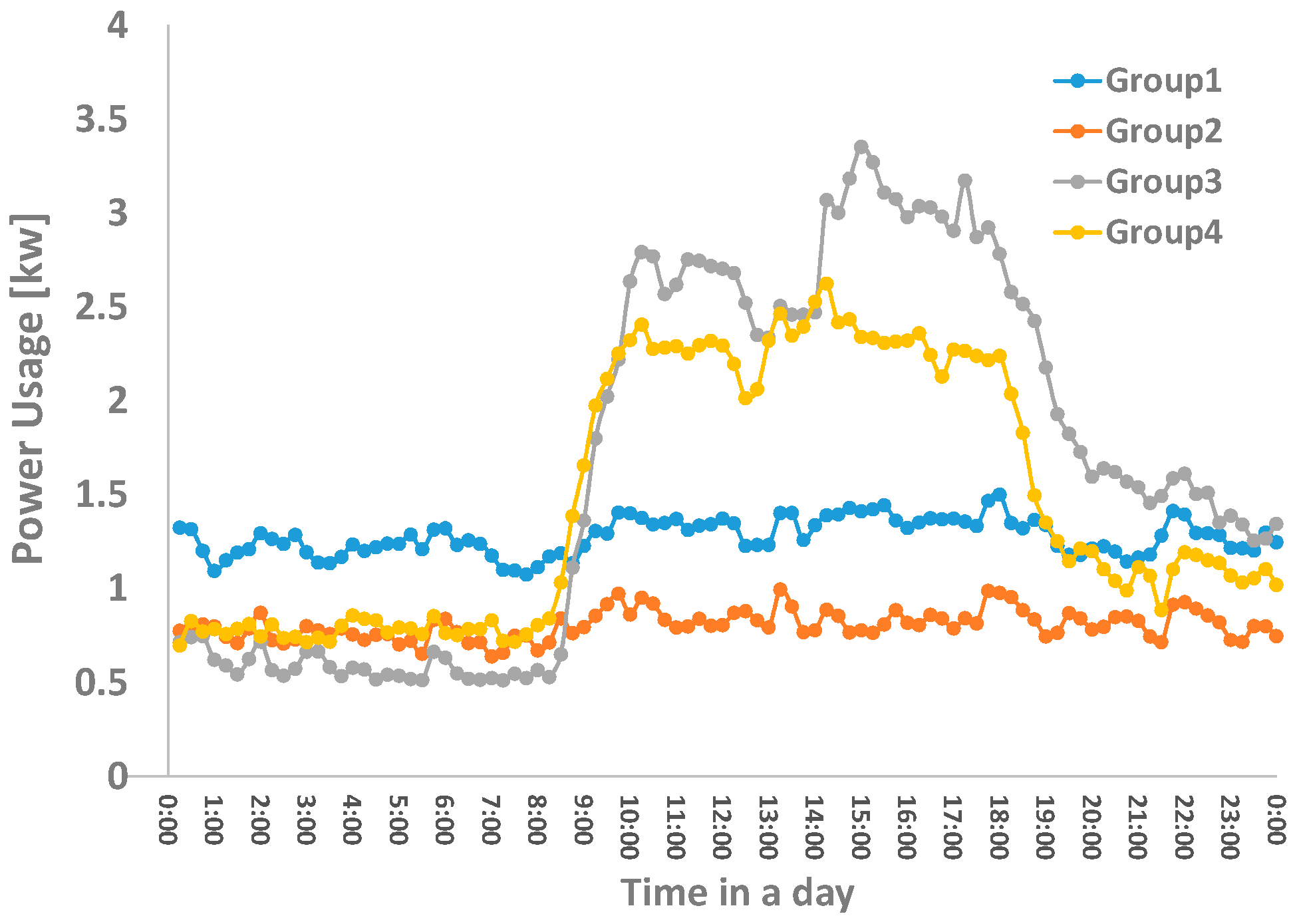
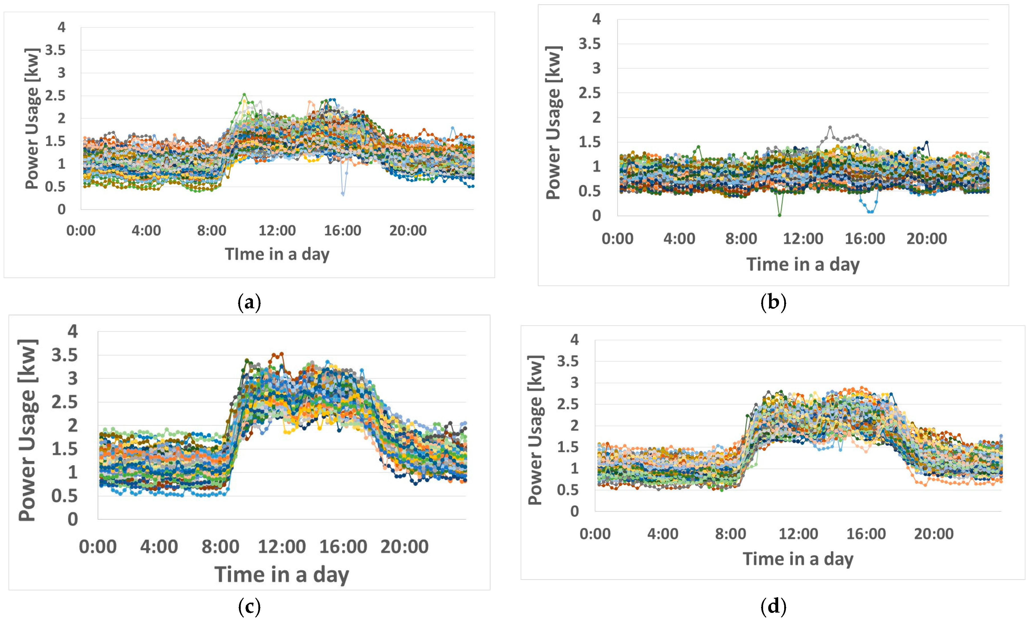
3.2.1. Classification of One-Year Data

An entire year of power usage data from one building in Korea was prepared. The load patterns are shown in Figure 9. This data set is composed of data recorded at 15-min intervals. k-means classification was adopted to classify similar days in a year. The number of classes k was chosen as four. Each group in Figure 10 is a good representation of the characteristic of load patterns to evaluate whether the proposed method would be able to effectively process various missing load patterns.

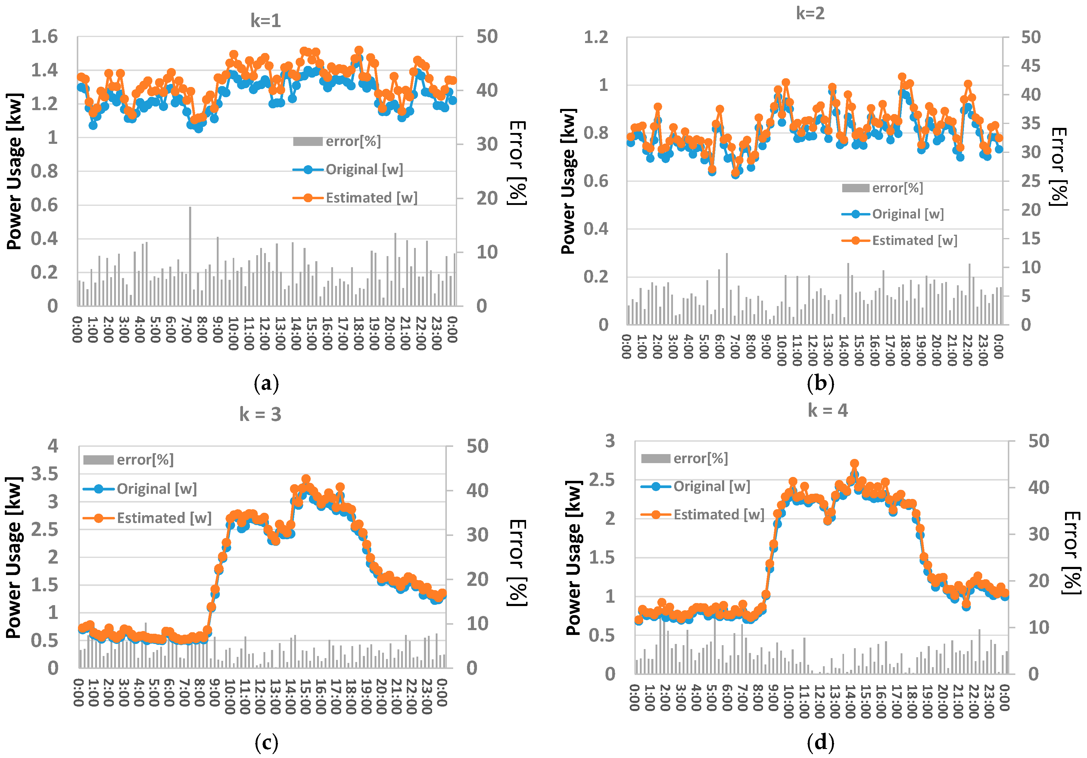
3.2.2. Validation of Estimation for Missing Meter Readings with Classified Load Data

The ability of the proposed method to process various load patterns was validated by extracting one of the classified load patterns from each group as representative of typical load patterns. The representative load patterns are shown in Figure 11. Figure 12 shows the result of the estimation for each group when the missing node is Node(2) in Figure 4. In every figure from (a) to (d) in Figure 12, the vertical axis on the left indicates the power usage missing from the data recorded on a day and estimated in this case study. The vertical axis on the right indicates the error rate of estimation, which is described by the bar graphs on the horizontal axis. Regarding all patterns from group1 to group4, the estimation error is approximately between 5% and 10%. In Figure 12, group3 and group4 have a relatively smaller error than group1 and group2. This is because more power usage data is missing from group3 and group4 than from group1 and group2. The other cases in which a missing meter node is located at the other T-nodes such as Node(4) and Node(10) are also validated. The estimation error throughout a day is summarized in

Table 2. MAPE of the estimation result for each estimation method.

	Group1			Group2			Group3			Group4
	Node(2)	Node(4)	Node(10)	Node(2)	Node(4)	Node(10)	Node(2)	Node(4)	Node(10)	Node(2)	Node(4)	Node(10)
MAPE (%)	4.46	6.77	4.88	5.32	5.21	5.32	4.20	4.35	4.82	3.91	4.45	4.85

. The estimation error of each group and missing node is approximately 5%, which indicates that the proposed method can estimate the missing readings regardless of the load patterns and location of the missing meter node.

4. Discussion

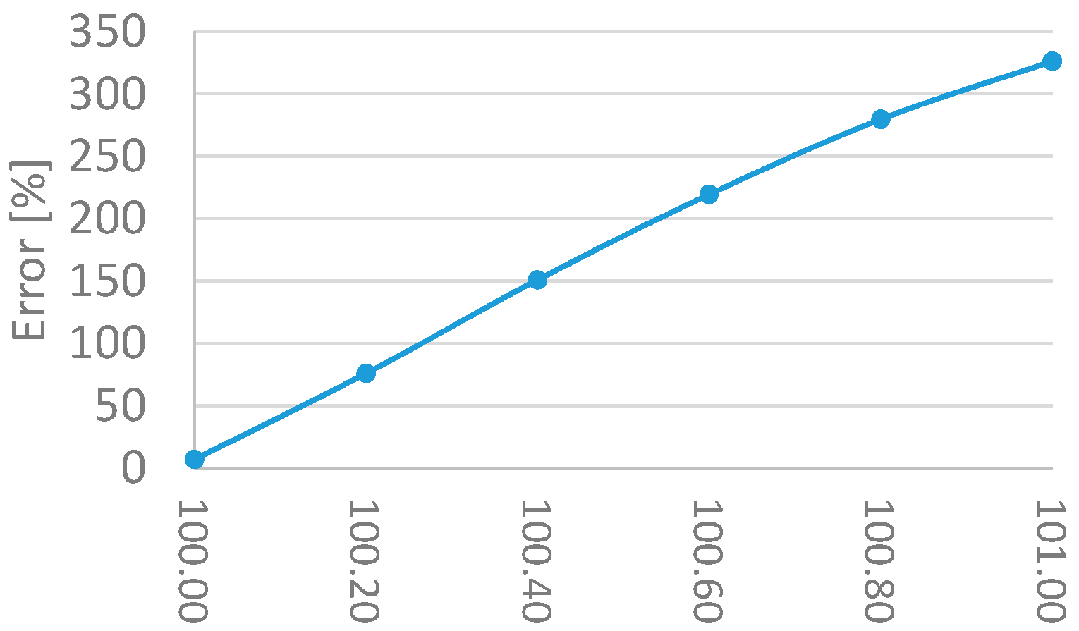
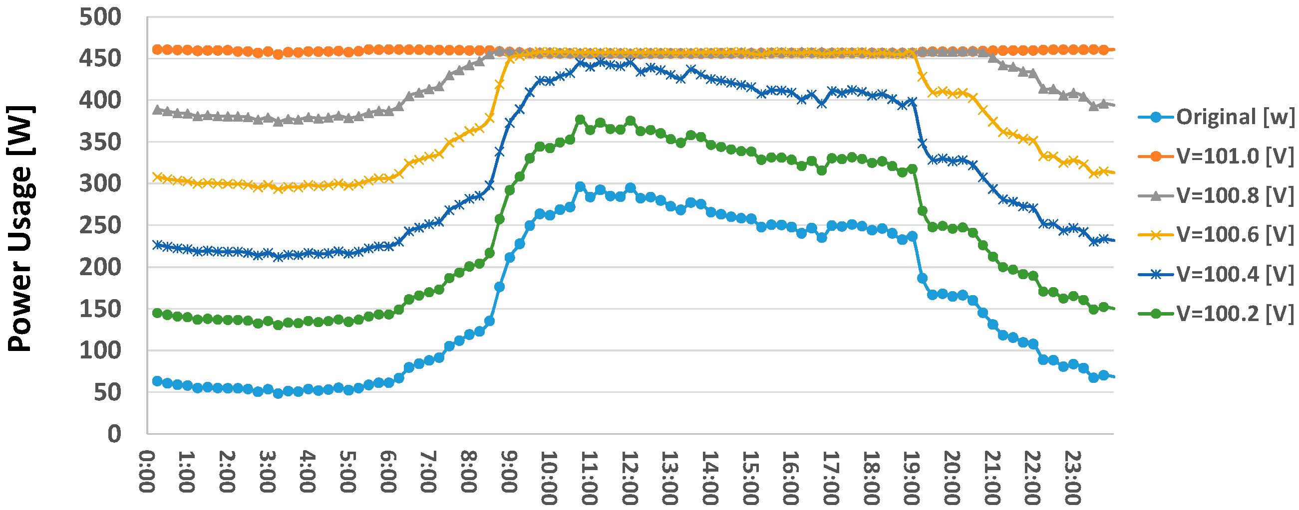
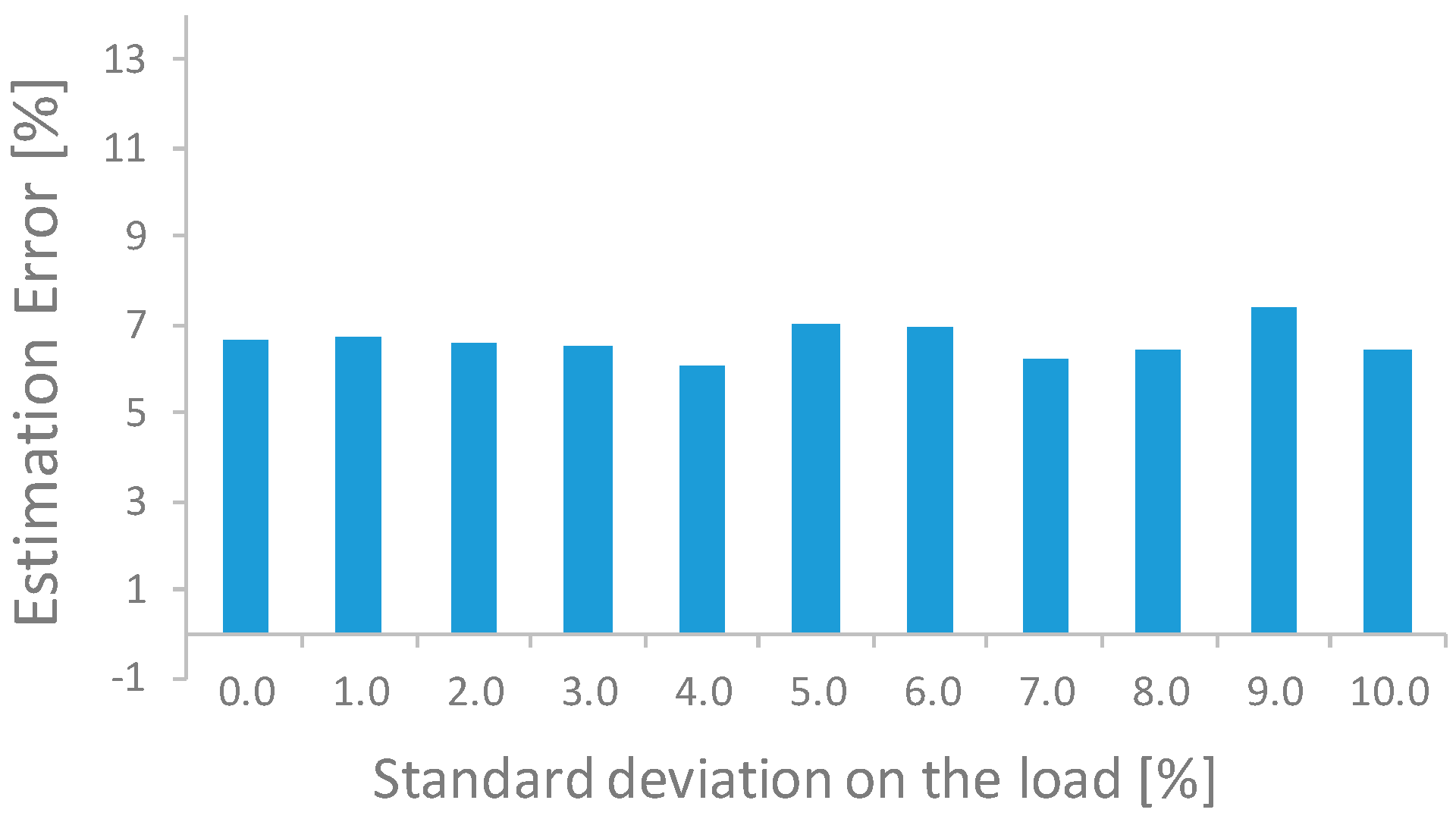
4.1. Evaluation of Robustness for Measurement Error

Especially, when the missing readings are observed at Node(2), as in Figure 4, the RMS voltage of the pole-transformer $V_{pole}$ should be known to calculate the missing readings. However, in the actual field at present, each pole-transformer cannot be expected to have a measurement device capable of measuring voltage and current. The secondary voltage of a pole-transformer is specified, e.g., 100 V or 200 V, which is not reliable as the real voltage because the primary side also has voltage fluctuations and the fluctuation affects the secondary side voltage. In this situation, state estimation in a high-voltage distribution network, which is on the primary side of a pole-transformer, can contribute to estimating the RMS voltage of the pole-transformer $|V_{pole}|$. Distribution system state estimators were proposed [30,31] and their robustness against the measurement error was evaluated. In these studies, the voltage of nodes containing the nodes at which the pole-transformer is located is estimated with various error rates. The assumed estimation error rate was found to be less than 1% when the aggregated power flow has a 3% measurement error [30]. Other researchers evaluated the voltage estimation error in a more realistic network along with load fluctuations [31]. The result shows that, with 1% measurement noise, the estimation error of the voltage magnitude is less than 1%. Therefore, in the following simulation, the accuracy of estimation of missing meter readings is evaluated while the estimated $|V_{pole}|$ has an error ranging from 0% to 1%. In this simulation, the true value of $|V_{pole}|$ is 100 V, but the true value is assumed to be unknown. It is assumed that $|V_{pole}|$ is estimated with an error such as 100.2, 100.4, …, 101.0 V. Figure 13 shows the estimation result of missing meter readings with the estimated value of $|V_{pole}|$. The original plot in the figure represents the missing readings to be estimated with the true value of $|V_{pole}|$. As shown in Figure 13, the estimated missing readings are as far as the estimated $|V_{pole}|$ from 100 V. When $|V_{pole}|=101.0$, the estimated missing meter readings closely approximate 450 W because of the current limitation. The error rate throughout a day is shown in Figure 14. The estimation error drastically increases as the estimated error with $|V_{pole}|$ increases. As shown in Figure 14, the error in the estimated $|V_{pole}|$ severely affects the accuracy of estimation of missing readings at the initial node. This relationship between the error in the estimated $|V_{pole}|$ and the estimation of missing readings is explained by the following equations.

$$V_{T2}+I_{T2}{Z}_{T2}-({\widehat{V}}_{T1}+{\widehat{I}}_{T1}{Z}_{T1})=0$$

(10)

$$|V_{pole}|-|V_{J2}+({\widehat{I}}_{T1}+I_{T2})Z_{J2}|=0$$

(11)

From Equation (11), the error in the estimated $|V_{pole}|$ is brought to ${\widehat{I}}_{T1}$ by multiplying with $Z_{J2}$, the value of which is generally assumed to be approximately 0.01. Therefore, even though the error contained in $|V_{pole}|$ is small, the error is multiplied by 100 and affects ${\widehat{I}}_{T1}$. A missing reading is calculated as ${\widehat{I}}_{T1}{\widehat{V}}_{T1}$. When ${\widehat{I}}_{T1}$ has an error that is 100 times larger, the estimated missing reading is also affected by an error that is 100 times larger. This is why even a small error in $|V_{pole}|$ causes a very large error with an estimated missing meter reading as shown in Figure 14. This problem remains a challenge as shown by the results presented in this paper.

4.2. Effect of Taking Average of One Minute

Here, the proposed method regards the load during one minute to be constant for the purpose of estimating the missing readings. However, strictly speaking, the actual load at every customer node (T-node) experiences variance even during a period of one minute. The following simulation evaluates the extent to which the load variance in one minute affects the estimation of missing readings. In the case of missing meter readings at Node(2), 10 fluctuated load patterns with standard deviations ranging from 0% to 10% are generated. Examples of these patterns for standard deviations ranging from 0% to 3% are shown in Figure 15. Figure 16 shows the result of missing reading estimation in terms of wh with respect to various fluctuating loads. As shown in Figure 16, the estimation error of wh during one minute is not significantly affected by the variance of the load.

5. Conclusions

This paper proposes a model-based method to infer missing smart meter readings by using the voltage and current information of neighboring nodes. Existing studies based on statistical inference methods such as data cleansing and NN-based methods cannot guarantee accuracy in the case in which readings are missing for longer periods and are not periodic. Case studies were used to estimate missing readings with and without outliers using the proposed method, the average method, and the NN-based method. In both of these case studies, the accuracy of the proposed method is superior to that of the other two methods. In addition, the proposed method was used with various load patterns. The simulation results confirmed that the proposed method can estimate the missing meter readings regardless of the missing load patterns. As for future works, estimation of missing readings under uncertainty from a network information perspective is considered. The topology of the lines in the low voltage distribution network is often not known. It is more prudent that the missing readings are estimated after an ambiguous topology is corrected with smart meter data.

References

1. Liang, X.; Li, X.; Lu, R.; Lin, X.; Shen, X. UDP: Usage-based dynamic pricing with privacy preservation for smart grid. IEEE Trans. Smart Grid 2013, 4, 141–150. [Google Scholar] [CrossRef]
2. Yoon, J.H.; Member, S.; Baldick, R.; Novoselac, A. Dynamic Demand Response Controller Based on Real-Time Retail Price for Residential Buildings. IEEE Trans. Smart Grid 2014, 5, 121–129. [Google Scholar] [CrossRef]
3. Hayes, B.; Melatti, I.; Mancini, T.; Prodanovic, M.; Tronci, E. Residential Demand Management using Individualised Demand Aware Price Policies. IEEE Trans. Smart Grid 2016, 8, 1284–1294. [Google Scholar] [CrossRef]
4. Chen, H.H.; Member, S.; Li, Y.; Member, S.; Louie, R.H.Y. Autonomous Demand Side Management Based on Energy Consumption Scheduling and Instantaneous Load Billing: An Aggregative Game Approach. IEEE Trans. Smart Grid 2014, 5, 1744–1754. [Google Scholar] [CrossRef]
5. Wei, C.; Member, S.; Fadlullah, Z. GT-CFS: A Game Theoretic Coalition Formulation Strategy for Reducing Power Loss in Micro Grids. IEEE Trans. Parallel Distrib. Syst. 2014, 25, 2307–2317. [Google Scholar] [CrossRef]
6. Peppanen, J.; Grimaldo, J.; Reno, M.J.; Grijalva, S.; Harley, R.G. Increasing Distribution System Model Accuracy with Extensive Deployment of Smart Meters. In Proceedings of the 2014 IEEE PES General Meeting, Conference & Exposition, National Harbor, MD, USA, 27–31 July 2014; pp. 1–5. [Google Scholar]
7. Alejandro, L.; Blair, C.; Bloodgood, L.; Khan, M.; Lawless, M. Global Market for Smart Electricity Meters: Government Policies Driving Strong Growth; Office of Industries U.S. International Trade Commission: Washington, DC, USA, 2014.
8. Sioshansi, F.P. Smart Grid: Integrating Renewable, Distributed and Efficient Energy, 1st ed.; Academic Press: New York, NY, USA, 2011. [Google Scholar]
9. Peppanen, J.; Reno, M.J.; Thakkar, M.; Grijalva, S.; Harley, R.G. Leveraging AMI Data for Distribution System Model Calibration and Situational Awareness. IEEE Trans. Smart Grid 2015, 6, 2050–2059. [Google Scholar] [CrossRef]
10. Haben, S.; Singleton, C.; Grindrod, P. Analysis and clustering of residential customers energy behavioral demand using smart meter data. IEEE Trans. Smart Grid 2016, 7, 136–144. [Google Scholar] [CrossRef]
11. Kavousian, A.; Rajagopal, R.; Fischer, M. Determinants of residential electricity consumption: Using smart meter data to examine the effect of climate, building characteristics, appliance stock, and occupants’ behavior. Energy 2013, 55, 184–194. [Google Scholar] [CrossRef]
12. Blair, S.M.; Booth, C.D.; Williamson, G.; Poralis, A.; Turnham, V. Automatically Detecting and Correcting Errors in Power Quality Monitoring Data. IEEE Trans. Power Deliv. 2016, 32, 1005–1013. [Google Scholar] [CrossRef]
13. Quilumba, F.L.; Lee, W.J.; Huang, H.; Wang, D.Y.; Szabados, R.L. Using smart meter data to improve the accuracy of intraday load forecasting considering customer behavior similarities. IEEE Trans. Smart Grid 2015, 6, 911–918. [Google Scholar] [CrossRef]
14. Wang, Y.; Zhang, N.; Chen, Q.; Kirschen, D.S.; Li, P.; Xia, Q. Data-Driven Probabilistic Net Load Forecasting with High Penetration of Invisible PV. IEEE Trans. Power Syst. 2017. [Google Scholar] [CrossRef]
15. Ding, N.; Benoit, C.; Foggia, G.; Bésanger, Y.; Member, S.; Wurtz, F. Neural Network-Based Model Design for Short-Term Load Forecast in Distribution Systems. IEEE Trans. Power Syst. 2016, 31, 72–81. [Google Scholar] [CrossRef]
16. Al-Wakeel, A.; Wu, J.; Jenkins, N. k-Means based load estimation of domestic smart meter measurements. Appl. Energy 2016, 194, 333–342. [Google Scholar] [CrossRef]
17. Xu, Y.; Dong, Z.Y.; Meng, K.; Wong, K.P.; Zhang, R. Short-term load forecasting of Australian National Electricity Market by an ensemble model of extreme learning machine. IET Gener. Transm. Distrib. 2013, 7, 391–397. [Google Scholar]
18. Li, S.; Wang, P.; Goel, L. A novel wavelet-based ensemble method for short-term load forecasting with hybrid neural networks and feature selection. IEEE Trans. Power Syst. 2016, 31, 1788–1798. [Google Scholar] [CrossRef]
19. Sun, X.; Luh, P.B.; Cheung, K.W.; Guan, W.; Michel, L.D.; Venkata, S.S.; Miller, M.T. An Efficient Approach to Short-Term Load Forecasting at the Distribution Level. IEEE Trans. Power Syst. 2016, 31, 2526–2537. [Google Scholar] [CrossRef]
20. Hayes, B.; Gruber, J.; Prodanovic, M. Short-Term Load Forecasting at the Local Level using Smart Meter Data. In Proceedings of the 2015 IEEE Eindhoven PowerTech, Eindhoven, The Netherlands, 29 June–2 July 2015. [Google Scholar]
21. Lork, C.; Zhou, Y.; Batchu, R.; Yuen, C.; Pindoriya, N.M. An Adaptive data driven approach to single unit residential air-conditioning prediction and forecasting using regression trees. In Proceedings of the 6th International Conference on Smart Cities and Green ICT Systems SMARTGREENS 2017, Porto, Portugal, 22–24 April 2017; pp. 67–76. [Google Scholar]
22. Weng, Y.; Negi, R.; Faloutsos, C.; Ilic, M.D. Robust Data-Driven State Estimation for Smart Grid. IEEE Trans. Smart Grid 2017, 8, 1956–1967. [Google Scholar] [CrossRef]
23. Barbeiro, P.N.P.; Teixeira, H.; Pereira, J.; Bessa, R. An ELM-AE State Estimator for real-time monitoring in poorly characterized distribution networks. In Proceedings of the 2015 IEEE Eindhoven PowerTech, Eindhoven, The Netherlands, 29 June–2 July 2015. [Google Scholar]
24. Chen, J.; Li, W.; Lau, A.; Cao, J.; Wang, K. Automated load curve data cleansing in power systems. IEEE Trans. Smart Grid 2010, 1, 213–221. [Google Scholar] [CrossRef]
25. Mateos, G.; Giannakis, G.B. Load Curve Data Cleansing and Imputation Via Sparsity and Low Rank. IEEE Trans. Smart Grid 2013, 4, 2347–2355. [Google Scholar] [CrossRef]
26. Han, S.; Kodaira, D.; Han, S.; Kwon, B.; Hasegawa, Y.; Aki, H. An Automated Impedance Estimation Method in Low-Voltage Distribution Network for Coordinated Voltage Regulation. IEEE Trans. Smart Grid 2016, 7, 1012–1020. [Google Scholar] [CrossRef]
27. Molina-Garcia, A.; Mastromauro, R.; Garcia-Sanchez, T.; Pugliese, S.; Liserre, M.; Stasi, S. Reactive Power Flow Control for PV Inverters Voltage Support in LV Distribution Networks. IEEE Trans. Smart Grid 2016, 8, 447–456. [Google Scholar] [CrossRef]
28. Demirok, E.; Sera, D.; Teodorescu, R.; Rodriguez, P.; Borup, U. Clustered PV inverters in LV networks: An overview of impacts and comparison of voltage control strategies. In Proceedings of the 2009 IEEE Electrical Power & Energy Conference (EPEC), Montreal, QC, Canada, 22–23 October 2009; pp. 1–6. [Google Scholar]
29. Hornik, K.; Stinchcombe, M.; White, H. Multilayer feedforward networks are universal approximators. Neural Netw. 1989, 2, 359–366. [Google Scholar] [CrossRef]
30. Nanchian, S.; Majumdar, A.; Pal, B.C. Ordinal Optimization Technique for Three Phase Distribution Network State Estimation Including Discrete Variables. IEEE Trans. Sustain. Energy 2017, 8, 1528–1535. [Google Scholar] [CrossRef]
31. Jia, Z.; Chen, J.; Liao, Y. State estimation in distribution system considering effects of AMI data. In Proceedings of the IEEE Southeastcon, Jacksonville, FL, USA, 4–7 April 2013. [Google Scholar]
Figure 1. Example of a missing reading in a secondary network.
Energies 11 00224 g001
Figure 2. Example of time-series active power data.
Energies 11 00224 g002
Figure 3. Generalized network model of a secondary distribution network.
Energies 11 00224 g003
Figure 4. Network consisting of five consuming nodes.
Energies 11 00224 g004
Figure 5. Load curve recorded during an entire day at a node with missing readings: (a) without outliers (b) with outliers.
Energies 11 00224 g005
Figure 6. Structure of estimation model based on NN.
Energies 11 00224 g006
Figure 7. Missing load curves recorded during an entire day and estimation results at Node(2): (a) Load without outliers; (b) Load with outliers.
Energies 11 00224 g007
Figure 8. MAPE and RMSE of the estimation result for each estimation method, where AV and NN denote the average and NN-based methods, respectively: (a) Load without outliers; (b) Load with outliers.
Energies 11 00224 g008
Figure 9. Load data from one building recorded in 2013, Korea.
Energies 11 00224 g009
Figure 10. Classified day loads of one building in 2013, Korea. (a) Group1, (b) Group2, (c) Group3 and (d) Group4 were generated by k-means clustering with k = 4 which provided the best accuracy for predicting the load data of 2014 for the same building.
Energies 11 00224 g010
Figure 11. Representative load patterns from each group classified by k-means classification.
Energies 11 00224 g011
Figure 12. Estimation result of missing meter readings at T-node(2) for each representative (a) Group1; (b) Group2; (c) Group3; and (d) Group4.
Energies 11 00224 g012
Figure 13. Estimation error of missing readings in initial part with respect to the error in the estimated voltage at the pole-transformer.
Energies 11 00224 g013
Figure 14. Estimation error of missing readings in initial part with respect to the error in the estimated voltage at the pole-transformer.
Energies 11 00224 g014
Figure 15. Examples of load fluctuations in one minute at Node(2).
Energies 11 00224 g015
Figure 16. Estimation error of missing readings with respect to variances.
Energies 11 00224 g016