Dynamic Strategies for Yaw and Induction Control of Wind Farms Based on Large-Eddy Simulation and Optimization


Abstract
1. Introduction
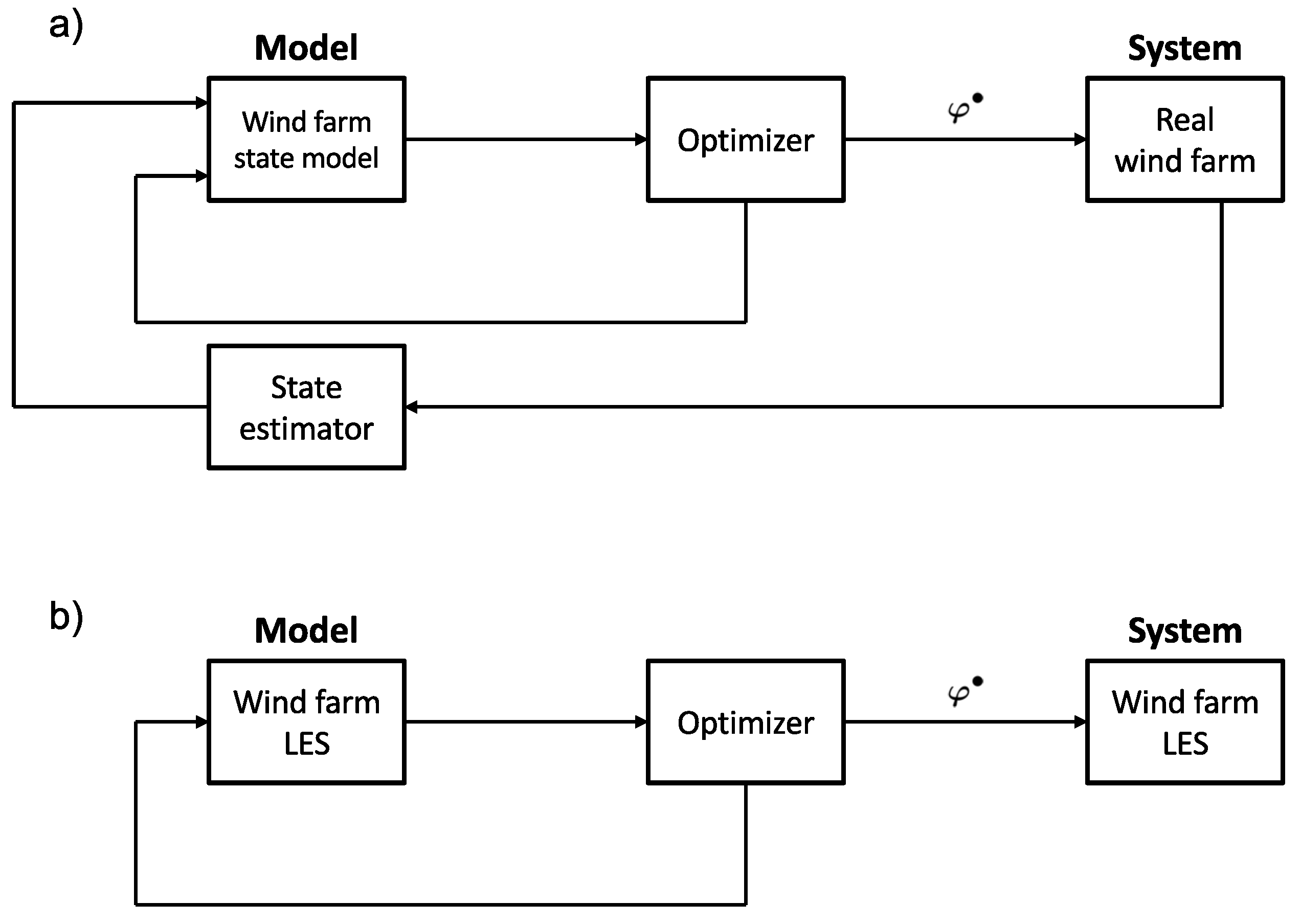
2. Methodology
3. Numerical Setup and Case Description
3.1. Simulation Setup
3.2. Control Cases
4. Results and Discussion
4.1. Convergence Behavior
4.2. Uniform Inflow
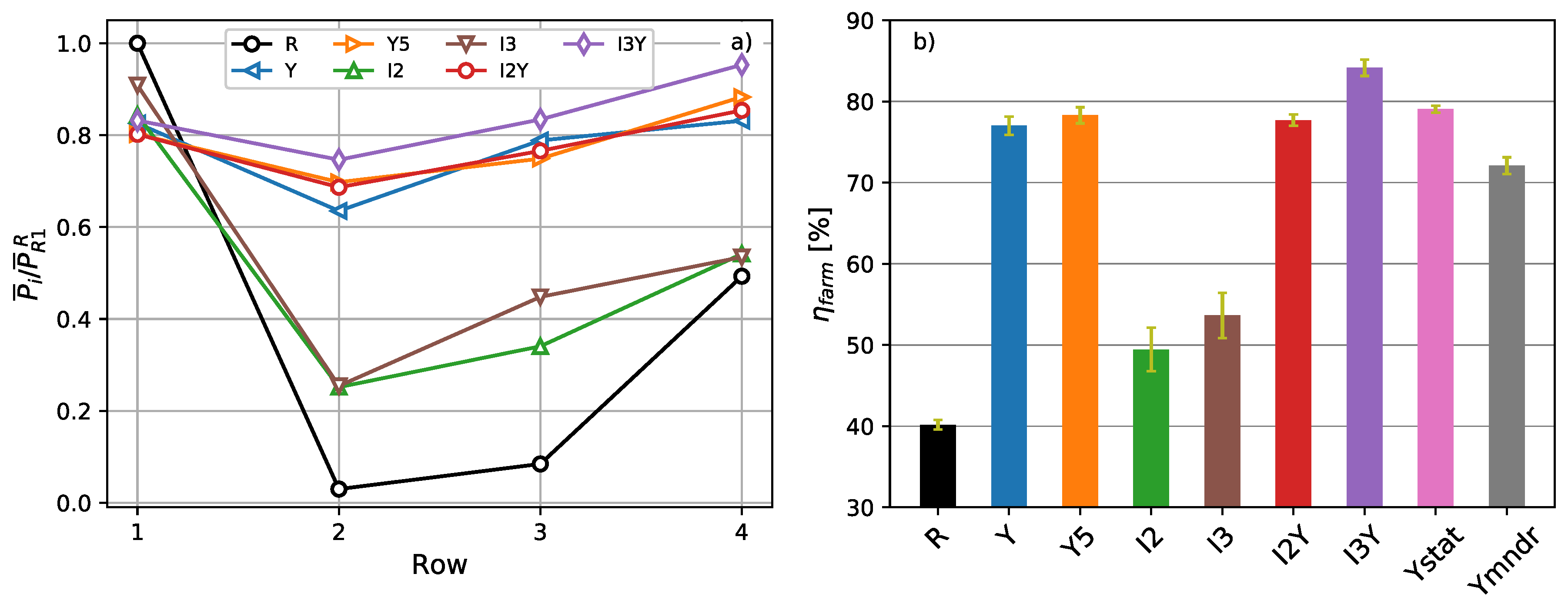
4.2.1. Power Extraction and Wind-Farm Efficiency
4.2.2. Yaw Characteristics
Static Yaw Regime—Wake Redirection
Dynamic Yaw Regime—Wake Meandering
4.2.3. Induction Characteristics
4.3. Turbulent Inflow
4.3.1. Power Extraction and Wind-Farm Efficiency
4.3.2. Yaw Characteristics
4.3.3. Induction Characteristics
4.4. Discussion
5. Conclusions and Future Work
Acknowledgments
Author Contributions
Conflicts of Interest
Appendix A. Derivation and Verification of the Adjoint Yaw Angle Equation and the Adjoint Gradient
Appendix A.1. Definition of Inner Products and Functional Gradients
Appendix A.2. Definition of Lagrangian Functional
Appendix A.3. Derivation of Adjoint Gradient
Appendix A.4. Derivation of Adjoint Yaw Angle Equation
Appendix A.4.1. Adjoint Disk Velocity Equation
Appendix A.4.2. Adjoint Rotor Footprint Equation
Appendix A.4.3. Adjoint Rotor-Perpendicular Vector Equation
Appendix A.4.4. Adjoint Yaw Angle Equation

Appendix A.5. Verification of Adjoint Gradient


References
- Boersma, S.; Doekemeijer, B.; Gebraad, P.; Fleming, P.; Annoni, J.; Scholbrock, A.; Frederik, J.; van Wingerden, J. A tutorial on control-oriented modeling and control of wind farms. In Proceedings of the 2017 IEEE American Control Conference (ACC), Seattle, WA, USA, 24–26 May 2017; pp. 1–18. [Google Scholar]
- Knudsen, T.; Bak, T.; Svenstrup, M. Survey of wind farm control—Power and fatigue optimization. Wind Energy 2015, 18, 1333–1351. [Google Scholar] [CrossRef]
- Annoni, J.; Gebraad, P.M.O.; Scholbrock, A.K.; Fleming, P.A.; Wingerden, J.W. Analysis of axial-induction-based wind plant control using an engineering and a high-order wind plant model. Wind Energy 2016, 19, 1135–1150. [Google Scholar] [CrossRef]
- Steinbuch, M.; de Boer, W.; Bosgra, O.; Peters, S.; Ploeg, J. Optimal control of wind power plants. J. Wind Eng. Ind. Aerodyn. 1988, 27, 237–246. [Google Scholar] [CrossRef]
- Horvat, T.; Spudić, V.; Baotić, M. Quasi-stationary optimal control for wind farm with closely spaced turbines. In Proceedings of the MIPRO, 2012 35th International Convention, Opatija, Croatia, 21–25 May 2012; pp. 829–834. [Google Scholar]
- Johnson, K.E.; Fritsch, G. Assessment of extremum seeking control for wind farm energy production. Wind Eng. 2012, 36, 701–715. [Google Scholar] [CrossRef]
- Gebraad, P.; Van Wingerden, J. Maximum power-point tracking control for wind farms. Wind Energy 2015, 18, 429–447. [Google Scholar] [CrossRef]
- Nilsson, K.; Ivanell, S.; Hansen, K.S.; Mikkelsen, R.; Sørensen, J.N.; Breton, S.P.; Henningson, D. Large-eddy simulations of the Lillgrund wind farm. Wind Energy 2015, 18, 449–467. [Google Scholar] [CrossRef]
- Campagnolo, F.; Petrović, V.; Bottasso, C.L.; Croce, A. Wind tunnel testing of wake control strategies. In Proceedings of the 2016 IEEE American Control Conference (ACC), Boston, MA, USA, 6–8 July 2016; pp. 513–518. [Google Scholar]
- Bartl, J.; Sætran, L. Experimental testing of axial induction based control strategies for wake control and wind farm optimization. J. Phys. Conf. Ser. 2016, 753, 032035. [Google Scholar] [CrossRef]
- Goit, J.P.; Meyers, J. Optimal control of energy extraction in wind-farm boundary layers. J. Fluid Mech. 2015, 768, 5–50. [Google Scholar] [CrossRef]
- Goit, J.P.; Munters, W.; Meyers, J. Optimal Coordinated Control of Power Extraction in LES of a Wind Farm with Entrance Effects. Energies 2016, 9, 29. [Google Scholar] [CrossRef]
- Munters, W.; Meyers, J. Effect of wind turbine response time on optimal dynamic induction control of wind farms. J. Phys. Conf. Ser. 2016, 753, 052007. [Google Scholar] [CrossRef]
- Munters, W.; Meyers, J. An optimal control framework for dynamic induction control of wind farms and their interaction with the atmospheric boundary layer. Philos. Trans. R. Soc. A 2017, 375. [Google Scholar] [CrossRef] [PubMed]
- Fleming, P.A.; Gebraad, P.M.; Lee, S.; van Wingerden, J.W.; Johnson, K.; Churchfield, M.; Michalakes, J.; Spalart, P.; Moriarty, P. Evaluating techniques for redirecting turbine wakes using SOWFA. Renew. Energy 2014, 70, 211–218. [Google Scholar] [CrossRef]
- Bossanyi, E. Individual blade pitch control for load reduction. Wind Energy 2003, 6, 119–128. [Google Scholar] [CrossRef]
- Fleming, P.; Gebraad, P.M.; Lee, S.; van Wingerden, J.W.; Johnson, K.; Churchfield, M.; Michalakes, J.; Spalart, P.; Moriarty, P. Simulation comparison of wake mitigation control strategies for a two-turbine case. Wind Energy 2015, 18, 2135–2143. [Google Scholar] [CrossRef]
- VerHulst, C.; Meneveau, C. Altering kinetic energy entrainment in large eddy simulations of large wind farms using unconventional wind turbine actuator forcing. Energies 2015, 8, 370–386. [Google Scholar] [CrossRef]
- Clayton, B.; Filby, P. Measured effects of oblique flows and change in blade pitch angle on performance and wake development of model wind turbines. In Proceedings of the 4th BWEA Wind Energy Conference, Stockholm, Sweden, 21–24 September 1982; Volume 13, pp. 559–572. [Google Scholar]
- Grant, I.; Parkin, P.; Wang, X. Optical vortex tracking studies of a horizontal axis wind turbine in yaw using laser-sheet, flow visualisation. Exp. Fluids 1997, 23, 513–519. [Google Scholar] [CrossRef]
- Medici, D.; Alfredsson, P.H. Measurements behind model wind turbines: Further evidence of wake meandering. Wind Energy 2008, 11, 211–217. [Google Scholar] [CrossRef]
- Bastankhah, M.; Porté-Agel, F. Experimental and theoretical study of wind turbine wakes in yawed conditions. J. Fluid Mech. 2016, 806, 506–541. [Google Scholar] [CrossRef]
- Jiménez, Á.; Crespo, A.; Migoya, E. Application of a LES technique to characterize the wake deflection of a wind turbine in yaw. Wind Energy 2010, 13, 559–572. [Google Scholar] [CrossRef]
- Howland, M.F.; Bossuyt, J.; Martínez-Tossas, L.A.; Meyers, J.; Meneveau, C. Wake structure in actuator disk models of wind turbines in yaw under uniform inflow conditions. J. Renew. Sustain. Energy 2016, 8, 043301. [Google Scholar] [CrossRef]
- Gebraad, P.; Teeuwisse, F.; Wingerden, J.; Fleming, P.A.; Ruben, S.; Marden, J.; Pao, L. Wind plant power optimization through yaw control using a parametric model for wake effects—A CFD simulation study. Wind Energy 2016, 19, 95–114. [Google Scholar] [CrossRef]
- Quick, J.; Annoni, J.; King, R.; Dykes, K.; Fleming, P.; Ning, A. Optimization Under Uncertainty for Wake Steering Strategies. J. Phys. Conf. Ser. 2017, 854, 012036. [Google Scholar] [CrossRef]
- Campagnolo, F.; Petrović, V.; Schreiber, J.; Nanos, E.M.; Croce, A.; Bottasso, C.L. Wind tunnel testing of a closed-loop wake deflection controller for wind farm power maximization. J. Phys. Conf. Ser. 2016, 753, 032006. [Google Scholar] [CrossRef]
- Park, J.; Kwon, S.D.; Law, K. A Data-Driven, Cooperative Approach for Wind Farm Control: A Wind Tunnel Experimentation. Energies 2017, 10, 852. [Google Scholar] [CrossRef]
- Soleimanzadeh, M.; Wisniewski, R.; Brand, A. State-space representation of the wind flow model in wind farms. Wind Energy 2014, 17, 627–639. [Google Scholar] [CrossRef]
- Fleming, P.; Annoni, J.; Shah, J.J.; Wang, L.; Ananthan, S.; Zhang, Z.; Hutchings, K.; Wang, P.; Chen, W.; Chen, L. Field test of wake steering at an offshore wind farm. Wind Energy Sci. 2017, 2, 229–239. [Google Scholar] [CrossRef]
- Gebraad, P.M.; Fleming, P.A.; van Wingerden, J.W. Wind turbine wake estimation and control using FLORIDyn, a control-oriented dynamic wind plant model. In Proceedings of the 2015 IEEE American Control Conference (ACC), Chicago, IL, USA, 1–3 July 2015; pp. 1702–1708. [Google Scholar]
- Park, J.; Law, K.H. Cooperative wind turbine control for maximizing wind farm power using sequential convex programming. Energy Convers. Manag. 2015, 101, 295–316. [Google Scholar] [CrossRef]
- Park, J.; Law, K.H. A data-driven, cooperative wind farm control to maximize the total power production. Appl. Energy 2016, 165, 151–165. [Google Scholar] [CrossRef]
- Delport, S.; Baelmans, M.; Meyers, J. Constrained optimization of turbulent mixing-layer evolution. J. Turbul. 2009, 10, N18. [Google Scholar] [CrossRef]
- Nita, C.; Vandewalle, S.; Meyers, J. On the efficiency of gradient based optimization algorithms for DNS-based optimal control in a turbulent channel flow. Comput. Fluids 2016, 125, 11–24. [Google Scholar] [CrossRef]
- Mehta, D.; van Zuijlen, A.H.; Koren, B.; Holierhoek, J.G.; Bijl, H. Large Eddy Simulation of wind farm aerodynamics: A review. J. Wind Eng. Ind. Aerodyn. 2014, 133, 1–17. [Google Scholar] [CrossRef]
- Sanderse, B.; van der Pijl, S.P.; Koren, B. Review of computational fluid dynamics for wind turbine wake aerodynamics. Wind Energy 2011, 14, 799–819. [Google Scholar] [CrossRef]
- Stevens, R.J.; Meneveau, C. Flow Structure and Turbulence in Wind Farms. Ann. Rev. Fluid Mech. 2017, 49, 311–339. [Google Scholar] [CrossRef]
- Munters, W.; Meneveau, C.; Meyers, J. Turbulent Inflow Precursor Method with Time-Varying Direction for Large-Eddy Simulations and Applications to Wind Farms. Bound. Layer Meteorol. 2016, 159, 305–328. [Google Scholar] [CrossRef]
- Meyers, J.; Sagaut, P. Evaluation of Smagorinsky variants in large-eddy simulations of wall-resolved plane channel flows. Phys. Fluids 2007, 19, 095105. [Google Scholar] [CrossRef]
- Meyers, J.; Meneveau, C. Large eddy simulations of large wind-turbine arrays in the atmospheric boundary layer. In Proceedings of the 48th AIAA Aerospace Sciences Meeting Including the New Horizons Forum and Aerospace Exposition, Orlando, FL, USA, 4–7 January 2010. [Google Scholar]
- Calaf, M.; Meneveau, C.; Meyers, J. Large eddy simulation study of fully developed wind-turbine array boundary layers. Phys. Fluids 2010, 22, 015110. [Google Scholar] [CrossRef]
- Byrd, R.H.; Lu, P.; Nocedal, J.; Zhu, C. A limited memory algorithm for bound constrained optimization. SIAM J. Sci. Comput. 1995, 16, 1190–1208. [Google Scholar] [CrossRef]
- Wolfe, P. Convergence conditions for ascent methods. SIAM Rev. 1969, 11, 226–235. [Google Scholar] [CrossRef]
- Jameson, A. Aerodynamic design via control theory. J. Sci. Comput. 1988, 3, 233–260. [Google Scholar] [CrossRef]
- Giles, M.B.; Pierce, N.A. An introduction to the adjoint approach to design. Flow Turbul. Combus. 2000, 65, 393–415. [Google Scholar] [CrossRef]
- Tröltzsch, F. Optimal control of partial differential equations. Grad. Stud. Math. 2010, 112. [Google Scholar] [CrossRef]
- Borzì, A.; Schulz, V. Computational Optimization of Systems Governed by Partial Differential Equations; Society for Industrial and Applied Mathematics (SIAM): Philadelphia, PA, USA, 2011. [Google Scholar]
- Bewley, T.R.; Moin, P.; Temam, R. DNS-based predictive control of turbulence: An optimal benchmark for feedback algorithms. J. Fluid Mech. 2001, 447, 179–225. [Google Scholar] [CrossRef]
- Choi, H.; Hinze, M.; Kunisch, K. Instantaneous control of backward-facing step flows. Appl. Numer. Math. 1999, 31, 133–158. [Google Scholar] [CrossRef]
- Munters, W.; Meneveau, C.; Meyers, J. Shifted periodic boundary conditions for simulations of wall-bounded turbulent flows. Phys. Fluids 2016, 28, 025112. [Google Scholar] [CrossRef]
- Martínez-Tossas, L.A.; Churchfield, M.J.; Meneveau, C. Large eddy simulation of wind turbine wakes: Detailed comparisons of two codes focusing on effects of numerics and subgrid modeling. J. Phys. Conf. Ser. 2015, 625, 012024. [Google Scholar] [CrossRef]
- Sarlak, H.; Meneveau, C.; Sørensen, J.N. Role of subgrid-scale modeling in large eddy simulation of wind turbine wake interactions. Renew. Energy 2015, 77, 386–399. [Google Scholar] [CrossRef]
- Troldborg, N.; Zahle, F.; Réthoré, P.; Sørensen, N. Comparison of wind turbine wake properties in non-sheared inflow predicted by different computational fluid dynamics rotor models. Wind Energy 2014, 18, 1239–1250. [Google Scholar] [CrossRef]
- Sarlak, H.; Pierella, F.; Mikkelsen, R.; Sørensen, J.N. Comparison of two LES codes for wind turbine wake studies. J. Phys. Conf. Ser. 2014, 524, 012145. [Google Scholar] [CrossRef]
- Ciri, U.; Rotea, M.; Santoni, C.; Leonardi, S. Large eddy simulation for an array of turbines with extremum seeking control. In Proceedings of the 2016 IEEE American Control Conference (ACC), Boston, MA, USA, 6–8 July 2016; pp. 531–536. [Google Scholar]
- Larsen, G.; Larsen, T.; Aagaard Madsen, H.; Mann, J.; Pena Diaz, A.; Barthelmie, R.; Jensen, L. The dependence of wake losses on atmospheric stability characteristics. In Extended Abstracts; Crespo, A., Larsen, G., Migoya, E., Eds.; Universidad Politecnica de Madrid: Madrid, Spain, 2009; pp. 35–37. [Google Scholar]
- Machefaux, E.; Larsen, G.C.; Koblitz, T.; Troldborg, N.; Kelly, M.C.; Chougule, A.; Hansen, K.S.; Rodrigo, J.S. An experimental and numerical study of the atmospheric stability impact on wind turbine wakes. Wind Energy 2016, 19, 1785–1805. [Google Scholar] [CrossRef]
- Jonkman, J.; Butterfield, S.; Musial, W.; Scott, G. Definition of a 5-MW Reference Wind Turbine for Offshore System Development; Technical Report Technical Report NREL/TP-500-38060; National Renewable Energy Laboratory: Golden, CO, USA, 2009.
- Kooijman, H.; Lindenburg, C.; Winkelaar, D.; van der Hooft, E. DOWEC 6 MW PRE-DESIGN: Aero-Elastic Modelling of the DOWEC 6 MW Pre-Design in PHATAS; Technical Report; Energy Research Center of the Netherlands (ECN): Petten, The Netherlands, 2003. [Google Scholar]
- Kim, M.G.; Dalhoff, P.H. Yaw Systems for wind turbines—Overview of concepts, current challenges and design methods. J. Phys. Conf. Ser. 2014, 524, 012086. [Google Scholar] [CrossRef]
- Munters, W. Large-Eddy Simulations and Optimal Coordinated Control of Wind-Farm Boundary Layers. Ph.D. Thesis, KU Leuven, Leuven, Belgium, 2017. [Google Scholar]
- Howard, K.B.; Singh, A.; Sotiropoulos, F.; Guala, M. On the statistics of wind turbine wake meandering: An experimental investigation. Phys. Fluids 2015, 27, 075103. [Google Scholar] [CrossRef]
- Allaerts, D.; Meyers, J. Boundary-layer development and gravity waves in conventionally neutral wind farms. J. Fluid Mech. 2017, 814, 95–130. [Google Scholar] [CrossRef]
- Cal, R.B.; Lebrón, J.; Castillo, L.; Kang, H.S.; Meneveau, C. Experimental study of the horizontally averaged flow structure in a model wind-turbine array boundary layer. J. Renew. Sustain. Energy 2010, 2, 013106. [Google Scholar] [CrossRef]
- Barthelmie, R.; Hansen, O.F.; Enevoldsen, K.; Hojstrup, J.; Frandsen, S.; Pryor, S.; Larsen, S.; Motta, M.; Sanderhoff, P. Ten years of meteorological measurements for offshore wind farms. J. Sol. Energy Eng. Trans. ASME 2005, 127, 170–176. [Google Scholar] [CrossRef]
- Barthelmie, R.J.; Hansen, K.; Frandsen, S.T.; Rathmann, O.; Schepers, J.; Schlez, W.; Phillips, J.; Rados, K.; Zervos, A.; Politis, E.; et al. Modelling and measuring flow and wind turbine wakes in large wind farms offshore. Wind Energy 2009, 12, 431–444. [Google Scholar] [CrossRef]
- Hinze, M.; Pinnau, R.; Ulbrich, M.; Ulbrich, S. Optimization with PDE Constraints; Springer Science & Business Media: Berlin, Germany, 2008; Volume 23. [Google Scholar]


| Simulation Parameters | ||||
| Domain size | km | |||
| Turbine dimensions | m | |||
| Turbine spacing | ||||
| Windfarm layout | turbines = 4 rows × 4 columns | |||
| Grid size | ||||
| Cell size | m | |||
| Time step | s | |||
| Uniform inflow | ||||
| Hub height | = 0.5 | |||
| Inflow velocity | = 8 m s | |||
| Turbulent inflow | ||||
| Hub height | = 0.1 | |||
| Precursor pressure gradient | m s | |||
| Surface roughness | m | |||
| Optimization Parameters | ||||
| Optimization method | L–BFGS–B | |||
| Hessian correction pairs | ||||
| BFGS iterations | ( PDE) | |||
| Optimization time window | s | |||
| Flow advancement time window | s | |||
| Total operation time | s (6 windows) | |||
| Cases | [] | |||
| Reference | (R) | 2 | 2 | 0 |
| Yaw control | (Y) | 2 | 2 | 0.3 |
| Fast yaw control | (Y5) | 2 | 2 | 5 |
| Underinduction control | (I2) | 0 | 2 | 0 |
| Overinduction control | (I3) | 0 | 3 | 0 |
| Underinduction + yaw control | (I2Y) | 0 | 2 | 0.3 |
| Overinduction + yaw control | (I3Y) | 0 | 3 | 0.3 |
| Control case | Abbreviation | ||
|---|---|---|---|
| Greedy control | |||
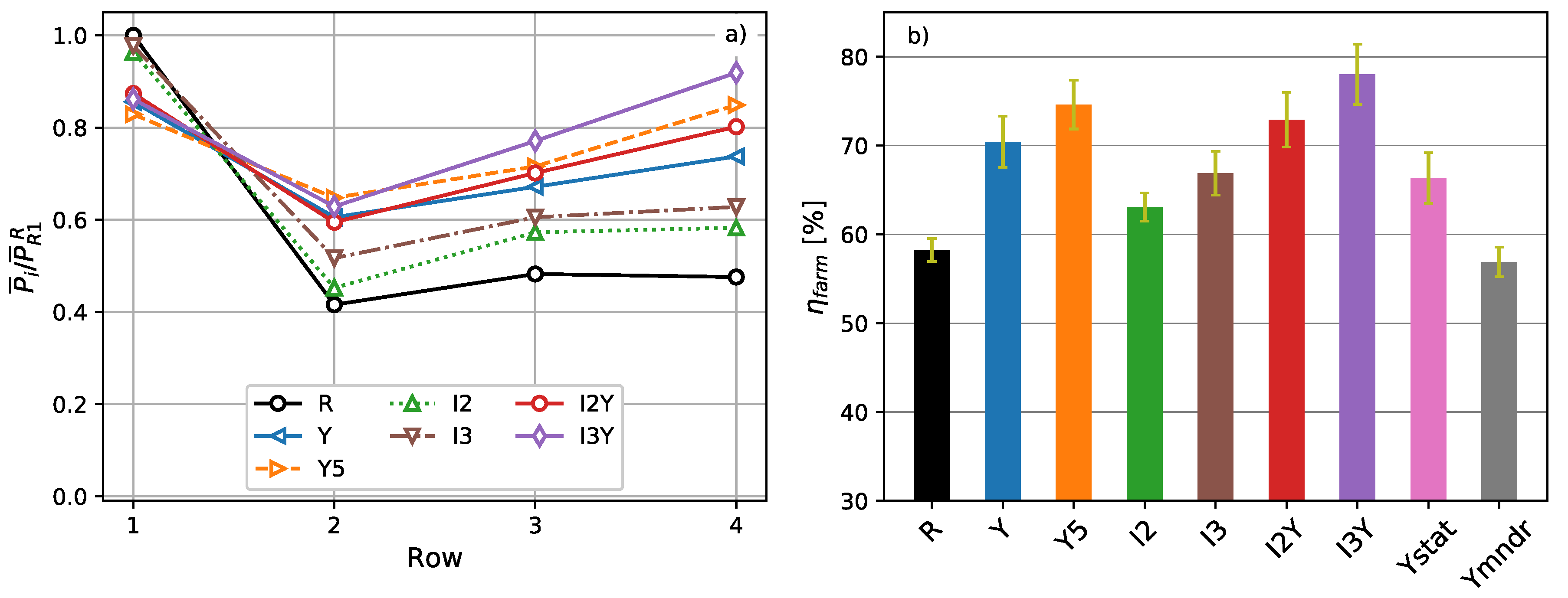
| Reference | R | 0.40 | 0.58 |
| Optimal control | |||
| Underinduction | I2 | 0.49 [+23%] | 0.63 [+8%] |
| Overinduction | I3 | 0.53 [+34%] | 0.67 [+15%] |
| Yaw | Y | 0.77 [+92%] | 0.70 [+21%] |
| Underinduction + yaw | I2Y | 0.77 [+93%] | 0.73 [+25%] |
| Fast yaw | Y5 | 0.78 [+95%] | 0.75 [+28%] |
| Overinduction + yaw | I3Y | 0.84 [+110%] | 0.78 [+34%] |
| Simplified control | |||
| Steady yaw | Ystat | 0.79 [+97%] | 0.66 [+14%] |
| Meandering yaw | Ymndr | 0.72 [+79%] | 0.57 [–2%] |
© 2018 by the authors. Licensee MDPI, Basel, Switzerland. This article is an open access article distributed under the terms and conditions of the Creative Commons Attribution (CC BY) license (http://creativecommons.org/licenses/by/4.0/).
Share and Cite
Munters, W.; Meyers, J. Dynamic Strategies for Yaw and Induction Control of Wind Farms Based on Large-Eddy Simulation and Optimization. Energies 2018, 11, 177. https://doi.org/10.3390/en11010177
Munters W, Meyers J. Dynamic Strategies for Yaw and Induction Control of Wind Farms Based on Large-Eddy Simulation and Optimization. Energies. 2018; 11(1):177. https://doi.org/10.3390/en11010177
Chicago/Turabian StyleMunters, Wim, and Johan Meyers. 2018. "Dynamic Strategies for Yaw and Induction Control of Wind Farms Based on Large-Eddy Simulation and Optimization" Energies 11, no. 1: 177. https://doi.org/10.3390/en11010177
APA StyleMunters, W., & Meyers, J. (2018). Dynamic Strategies for Yaw and Induction Control of Wind Farms Based on Large-Eddy Simulation and Optimization. Energies, 11(1), 177. https://doi.org/10.3390/en11010177