Thermal Impact Assessment of Groundwater Heat Pumps (GWHPs): Rigorous vs. Simplified Models

Abstract

Groundwater Heat Pumps (GWHPs) are increasingly adopted for air conditioning in urban areas, thus reducing CO₂ emissions, and this growth needs to be managed to ensure the sustainability of the thermal alteration of aquifers. However, few studies have addressed the propagation of thermal plumes from open-loop geothermal systems from a long-term perspective. We provide a comprehensive sensitivity analysis, performed with numerical finite-element simulations, to assess how the size of the thermally affected zone is driven by hydrodynamic and thermal subsurface properties, the vadose zone and aquifer thickness, and plant setup. In particular, we focus the analysis on the length and width of thermal plumes, and on their time evolution. Numerical simulations are compared with two simplified methods, namely (i) replacing the time-varying thermal load with its yearly average and (ii) analytical formulae for advective heat transport in the aquifer. The former proves acceptable for the assessment of plume length, while the latter can be used to estimate the width of the thermally affected zone. The results highlight the strong influence of groundwater velocity on the plume size and, especially for its long-term evolution, of ground thermal properties and of subsurface geometrical parameters.

1. Introduction

Ground Source Heat Pumps (GSHPs) utilize the ground as a heat source or sink, respectively, for the heating or cooling of buildings. At moderate depths (5 to 20 m), the ground has an almost constant temperature, with a value close to the yearly average air temperature [1]; hence, GSHPs have a higher energy efficiency (coefficient of performance, COP) compared to Air Source Heat Pumps (ASHPs) [2], and their potential for the reduction of the carbon intensity of building air conditioning is widely acknowledged [3].

The energy efficiency of a GSHP strongly depends on site-specific properties of the ground, for both Borehole Heat Exchangers (BHEs) [4,5,6,7,8] and Ground Water Heat Pumps (GWHPs) [9,10,11,12]. GWHPs exchange heat with groundwater extracted through one or multiple water wells, and are increasingly employed as an air conditioning system, especially for large commercial and public buildings [13,14,15,16]. Groundwater is usually reinjected through wells into the same aquifer to avoid its depletion [17], but this leads to the formation of thermally altered zones, called thermal plumes. Thermal plumes pose two sustainability issues: the upstream propagation of the plume, which can reach the abstraction well (thermal short-circuit) [9,18,19], thus reducing the COP of the heat pump, and the downstream propagation of the plume, which can impair drinking water wells or other GWHPs. Assessing the subsurface thermal impact of open-loop geothermal systems is therefore essential for their design.

Temperature changes in aquifers induced by open-loop well doublets have been extensively investigated in past decades [20,21]. Simple cases can be solved using analytical formulae, while numerical models are used to obtain more reliable estimations of thermal plume size in more complex scenarios, although they are more expensive and time consuming. Banks [22] derived 2D analytical solutions for thermal plume estimation in the case of a well doublet aligned with the groundwater flow direction, starting from the general solutions provided by Shan [23] and by Luo and Kitanidis [24]. Milnes and Perrochet [25] defined thermal recycling and feedback, and derived mathematical formulae for the calculation of the maximum thermal alteration of the abstracted groundwater. Lippmann [21] provided an analytical solution for thermal feedback, while Casasso and Sethi [9] developed the numerical code TRS (Thermal Recycling Simulator) and an empirical formula for the estimation of thermal recycling in open-loop well doublets. A number of numerical models of thermal plume propagation are also available in the literature, applied to both single plants [14,26,27,28] and systems at an urban scale for the resolution of territorial planning issues [29,30,31].

These papers deal with specific case studies, but few works assess the influence of thermal, hydrogeological, and operational parameters on thermal plumes in a general way. Lo Russo et al. [32] performed a sensitivity analysis on an open-loop system in the aquifer of Turin (Northern Italy) considering a ±20% variation on the design values of various aquifer thermal and hydrodynamic parameters, with a one-year simulation time. They found that the dimensions of the thermal plume are most sensitive to the hydraulic conductivity, the hydraulic gradient and, to a lesser extent, the thermal capacity of the aquifer. Bridger and Allen [27] studied an Aquifer Thermal Energy Storage (ATES) in a layered geological setup, concluding that anisotropy of the hydraulic conductivity and of the hydraulic gradient exert the greatest influence on the propagation of the thermal plume. The main limitations of these studies are the narrow variation ranges considered for these parameters and the short simulated operating times, relative to the time scales of thermal plume evolution.

The purpose of the first part of this work is to fill this gap by comparing, by means of a parametric sweep study, the relative influence of hydrodynamic, thermal, and geometrical parameters of the aquifer and technical-operating parameters of the plant on the long-term propagation of the thermal plumes generated by an open-loop well doublet.

The second part of the paper is devoted to the evaluation of different methods to estimate the size of the thermal plume. Three different approaches for plume estimation were tested and, by comparing the results, we defined the conditions for which errors introduced by approximated numerical and analytical solutions are acceptable. The first, and most accurate, method used in this study is a finite element numerical flow and heat-transport simulation with a sinusoidal heating and cooling thermal load to reproduce the typical trend of a building’s energy demand through the year. The second method involves the simplifying assumption of a constant thermal load, derived from the balance between the yearly heating and cooling demand. This is a common approach adopted, for instance, by the software GED (Groundwater Energy Designer) [33]. The third method is based on 2D analytical formulae provided by Banks [22], which allow for a rough estimation of the magnitude of thermally affected areas. This method is expected to be the least accurate, as the effects of many parameters involved in underground heat transfer are neglected.

The well doublet considered in our analysis is aligned with the large-scale groundwater flow direction, which is the best well arrangement to avoid or limit thermal recycling [18]. Starting from a default configuration, a parametric sweep was performed, determining the plume size for each simulation. Unlike most of the aforementioned studies, a long simulation time (50 years) was chosen to study the long-term response of the aquifer. The variations in the thermal plume’s length and width allow to assess the relative importance of each subsurface parameter, and to define the margins of error deriving from their approximate estimation.

2. Methods

2.1. Flow and Heat-Transport in Porous Media

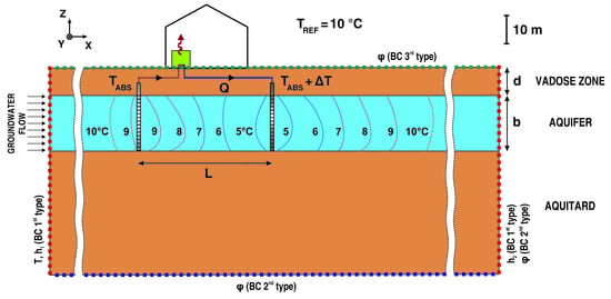
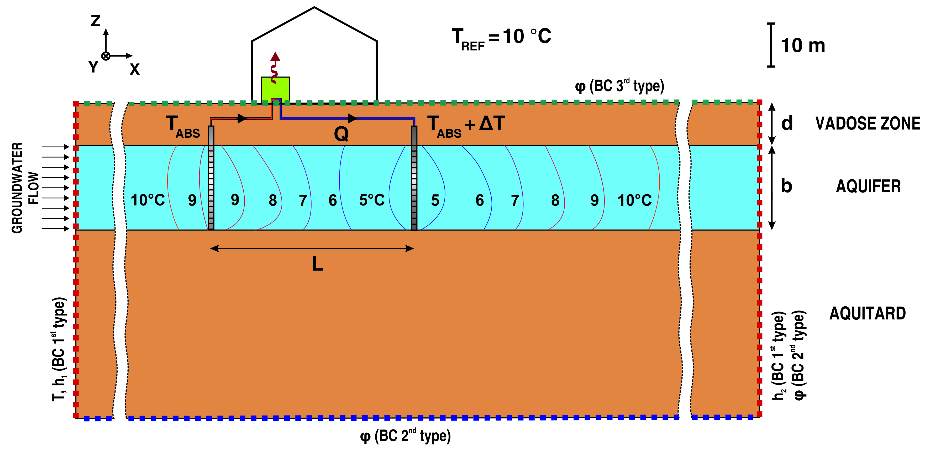
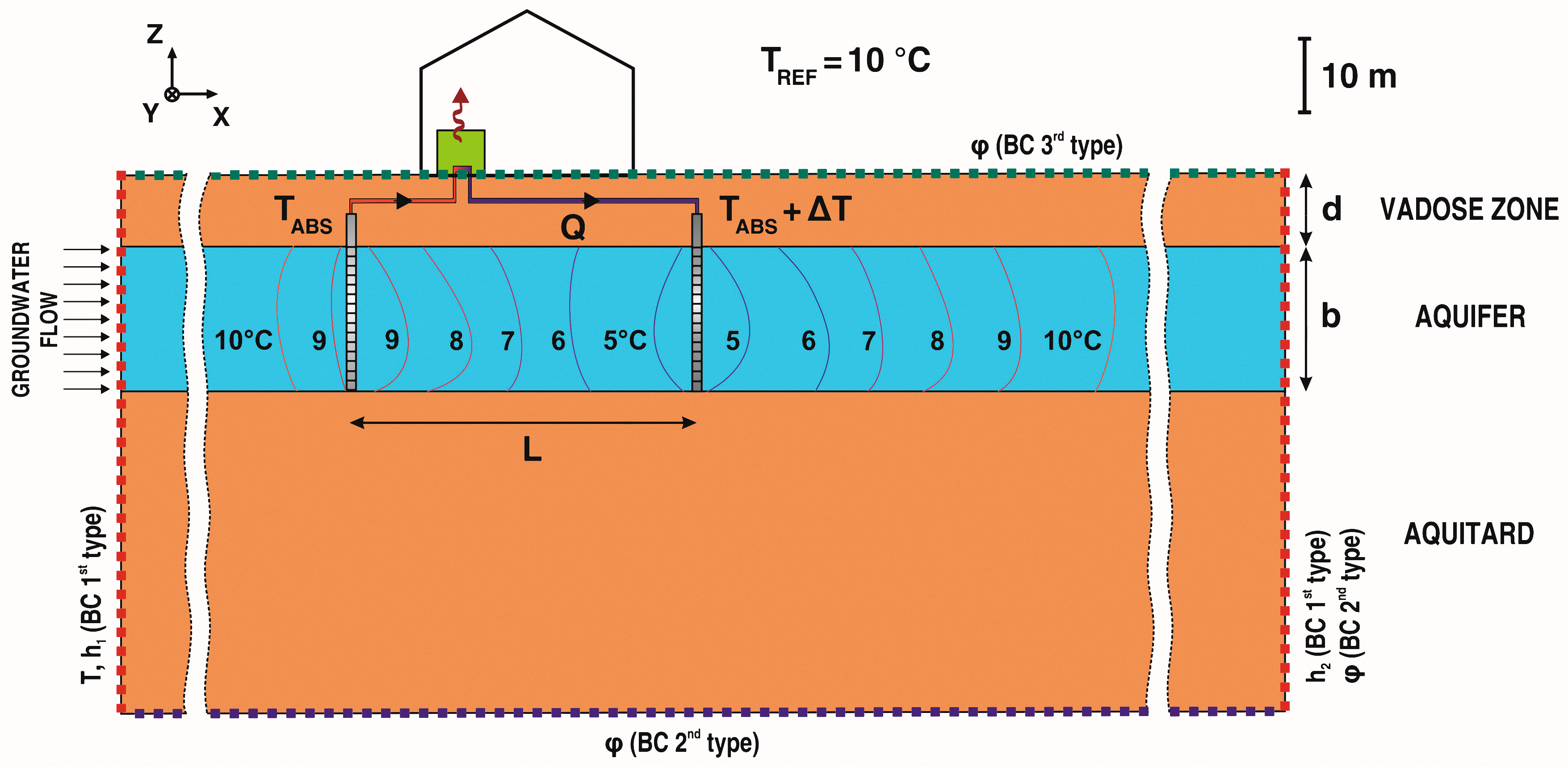
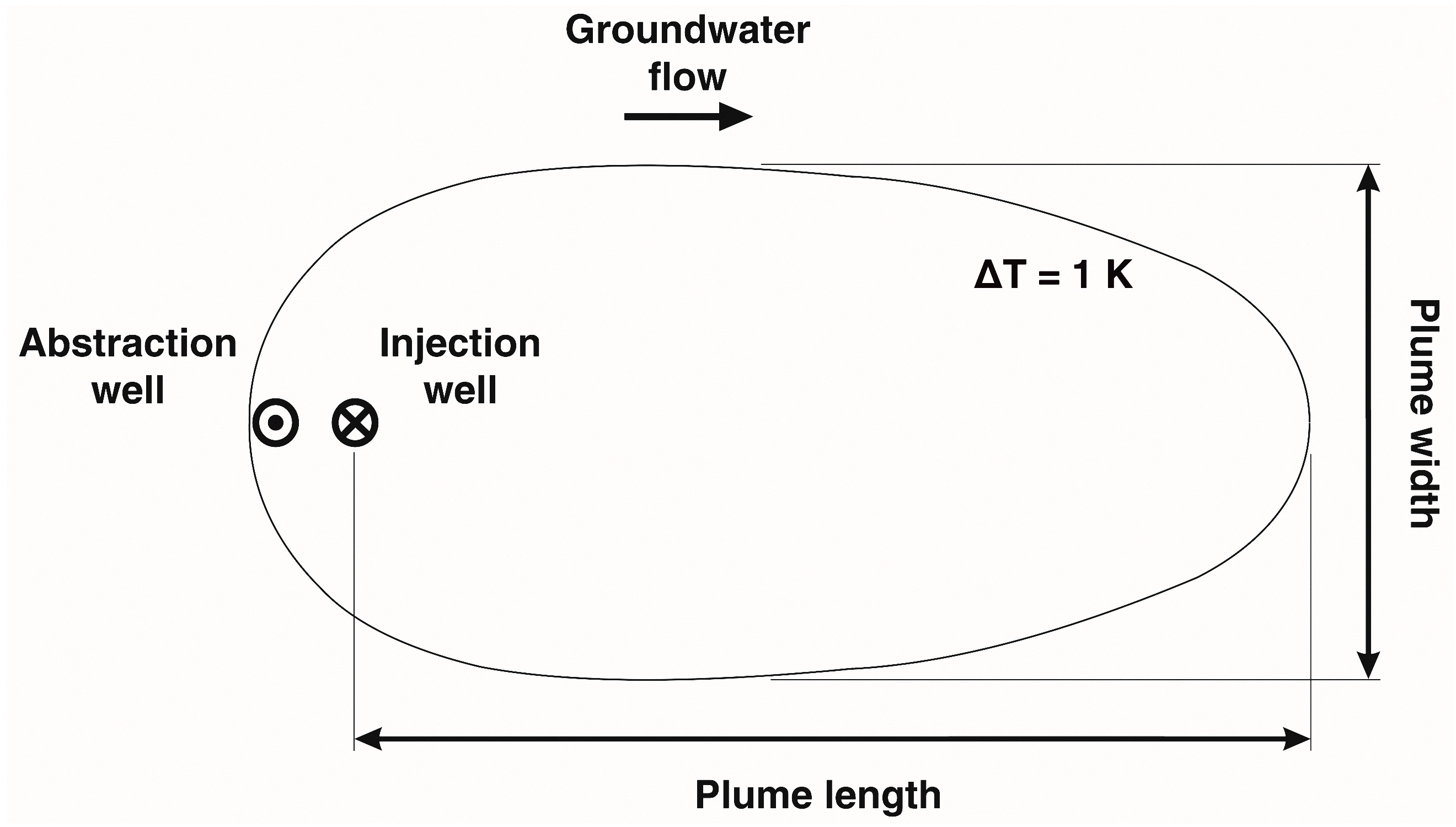
Heat transport in saturated porous media occurs by conduction (driven by temperature gradient), advection (due to the flow of the fluid phase), and dispersion (induced by the heterogeneity of the groundwater velocity field).

These mechanisms are described by the heat conservation equation in a two-phase (solid and liquid) medium [34], with the assumption of a groundwater flow aligned with the x-axis:

$$\rho c\frac{\partial T}{\partial t}+{\rho }_w{c}_w{v}_D\frac{\partial T}{\partial x}+\left(\lambda +{\rho }_w{c}_w{v}_D{\alpha }_L\right)\frac{{\partial }^{2}T}{\partial x^2}+\left(\lambda +{\rho }_w{c}_w{v}_D{\alpha }_T\right)\left(\frac{{\partial }^{2}T}{\partial y^2}+\frac{{\partial }^{2}T}{\partial z^2}\right)=H$$

(1)

where $\rho c$ and ${\rho }_w{c}_w$ are the thermal capacities (J·m⁻³·K⁻¹) of the porous medium and of the liquid phase, respectively; $T$ is the temperature (K), considered equal for the solid and the liquid phases (i.e., the thermal equilibrium is considered instantaneous); $v_D$ is the Darcy velocity (m·s⁻¹); ${\alpha }_L$ and ${\alpha }_T$ are, respectively, the longitudinal and transverse dispersivities (m) relative to the groundwater flow direction; $\lambda$ is the thermal conductivity of the porous medium (W·m⁻¹·K⁻¹); and $H$ is the heat source/sink (W·m⁻³).

The first term of Equation (1) is the temperature variation over time, which depends on the volume-averaged (bulk) heat capacity of the porous medium ($\rho c$):

$$\rho c=n_e{\rho }_w{c}_w+\left(1-n_e\right){\rho }_s{c}_s$$

(2)

where ${\rho }_s{c}_s$ is the thermal capacity (J·m⁻³·K⁻¹) of the solid phase.

The second term describes the advection, which is function of the Darcy velocity ($v_D$):

$$v_D=-K\frac{\partial h}{\partial x}=-Ki$$

(3)

where $K$ is the hydraulic conductivity (m·s⁻¹), $h$ is the hydraulic head (m), and $i$ is the hydraulic gradient along the x direction (dimensionless).

Conduction depends on the bulk thermal conductivity in the third term of Equation (1):

$$\lambda =\left(1-n_e\right){\lambda }_s+n_e{\lambda }_w$$

(4)

where ${\lambda }_s$ and ${\lambda }_w$ are the thermal conductivities (W·m⁻¹·K⁻¹) of, respectively, the solid matrix and the groundwater, and $n_e$ is the effective porosity (dimensionless).

Thermal dispersion is described in Equation (1) by the corresponding coefficients ${\alpha }_L$ and ${\alpha }_T$. Dividing Equation (1) by $\rho c$, we get:

$$\frac{\partial T}{\partial t}+\frac{v_e}{R_{th}}\frac{\partial T}{\partial x}+D_x\frac{{\partial }^{2}T}{\partial x^2}+D_y\frac{{\partial }^{2}T}{\partial y^2}+D_z\frac{{\partial }^{2}T}{\partial z^2}=\frac{H}{\rho c}$$

(5)

where $v_e$ is the effective velocity of groundwater through the pores, calculated as:

$$v_e=\frac{v_D}{n_e}$$

(6)

Since heat is exchanged between the fluid and the solid phase, the advective velocity of the thermal plume is lower than the groundwater flow velocity [19]. This phenomenon is similar to solute sorption in porous media with linear kinetics. By analogy, it is therefore possible to define the thermal retardation coefficient of Equation (5) as the ratio between the effective velocity of groundwater ($v_e$) and heat front ($v_{th}$):

$$R_{th}=\frac{v_e}{v_{th}}=\frac{\left(1-n_e\right){\rho }_s{c}_s+n_e{\rho }_w{c}_w}{n_e{\rho }_w{c}_w}=\frac{\rho c}{n_e{\rho }_w{c}_w}$$

(7)

${\mathrm{D}}_x$, ${\mathrm{D}}_y$, and ${\mathrm{D}}_z$ are the longitudinal and transversal thermal dispersion coefficients (m²/s):

$${\mathrm{D}}_x=\frac{\lambda }{\rho c}+\frac{v_e}{R_{th}}{\alpha }_L$$

(8)

$${\mathrm{D}}_y={\mathrm{D}}_z=\frac{\lambda }{\rho c}+\frac{v_e}{R_{th}}{\alpha }_T$$

(9)

2.2. Model Setup

The objective of the first part of this work is to evaluate and compare the influence of thermal and hydrogeological subsurface properties (i.e., hydraulic conductivity of the aquifer, $K$; hydraulic gradient, $i$; effective porosity, $n_e$; aquifer and vadose zone thickness, $b$ and $d$, respectively; thermal capacity $\rho c$), as well as plant parameters (i.e., well spacing $L$), on the time evolution and spatial distribution of the thermal plume originated by a GWHP.

A simple but representative plant configuration was therefore adopted for the simulations, i.e., a well doublet in an unconfined aquifer, where the wells are aligned with the groundwater flow direction and the reinjection well is downstream of the abstraction well. The open-loop geothermal system was modelled with the finite-element code FEFLOW^® 6.2 (DHI-WASY, Berlin, Germany) [34], performing transient coupled flow and heat-transport simulations over an operating lifetime of 50 years. The default dimensions of the 3D modelling domain are 6000 m × 3000 m × 75 m, and variations were introduced only in the mesh thickness. The default vertical discretization is of 15 horizontal layers (16 slices), yielding a triangular mesh of 461,850 elements and 252,144 nodes for the default well configuration (Figure S1 in the Supplementary Materials), with slight variations for the others. A mesh density convergence study was performed (Figure S2 in the Supplementary Materials. The layers crossing the vadose zone, the aquifer, and the upper part of the underlying aquitard (layers 1 to 13) have a constant thickness of 2.5 m. The bottom two layers are thicker (10 m and 30 m, respectively), since this portion is deemed to be negligibly affected by the GWHP.

A simplified 2D cross-section of the model is shown in Figure 1.

The regional groundwater flow was reproduced by assigning constant hydraulic head values (hydraulic boundary condition (BC) of the first kind) on the western (upgradient) and eastern (downgradient) domain borders, based on both the aquifer thickness and the hydraulic gradient. Hydraulic head initial conditions were then assigned by running the model in steady state conditions and flow-only mode, without pumping wells. Two water wells, one for abstraction and one for reinjection, were implemented in the model as a Multi-layer Well (flow BC of the fourth kind, according to [34]) screened over the total aquifer thickness. The abstraction well was placed at coordinates x, y (1000; 1500) m, in order to allow the thermal plume to propagate entirely inside the domain, while the reinjection well was located downgradient at a selected distance from the abstraction wells. The well radius was set equal to 0.25 m, a typical value for wells operating at the flow rates considered in this work.

The thermal balance of the aquifer was reproduced by imposing the undisturbed aquifer temperature (assumed equal to 10 °C) on the upstream side of the domain (first kind BC). On the top slice, the heat exchange with the external air was reproduced imposing a Cauchy boundary condition of the third kind [35], i.e., a heat flux proportional to the difference relative to the above-mentioned reference temperature (10 °C). The geothermal temperature gradient was not taken into account, since its effect is usually negligible at depths between 30 m and 50 m [36,37,38,39]; hence, a null heat flux (second kind BC) was imposed on the lowest slice. The same BC was applied to the remaining domain borders. Consistently with the heat boundary conditions, an initial temperature of 10 °C was assigned to the whole domain.

The operation of the GWHP was simulated by imposing a constant temperature difference ($\Delta T=T_{inj}-T_{abs}$) of ±4 °C between the injection and abstraction wells (negative when heating and positive when cooling). The flow rate $Q\left(t\right)$ varies with the thermal load $P\left(t\right)$ exchanged with the groundwater according to the following equation:

$$P\left(t\right)={\rho }_w{c}_w·Q\left(t\right)·\Delta T$$

(10)

The yearly evolution of $P\left(t\right)$ follows a sinusoidal trend, as shown in Figure 2. The thermal load is negative when heat is extracted from groundwater, and positive when heat is injected. Details on the model validation are available in the Supplementary Materials.

Using this model setup, a parametric sweep study was performed starting from a default setup and varying one parameter value per simulation.

Table 1. Parameter values assigned in the simulations.

Parameter	Symbol	Unit	Adopted Values	Default Value
Aquifer hydraulic conductivity	$K_{xx};K_{yy}$	m·s−1	5 × 10−4, 10−3, 5 × 10−3, 10−2	10−3
	$K_{zz}=0.1K_{xx}$		5 × 10−5, 10−4, 5 × 10−4, 10−3	10−4
Hydraulic gradient	$i$	10−3	1, 2, 4, 6, 10	2
Darcy velocity	$v_D$	m·s−1	10−6, 2 × 10−6, 5 × 10−6, 10−5, 2 × 10−6	2 × 10−6
Effective porosity	$n_e$	-	0.1, 0.2, 0.3	0.2
Thermal dispersivity	${\alpha }_L$	m	0.5, 2, 10, 50	10
	${\alpha }_T=0.1{\alpha }_L$		0.05, 0.2, 1, 5
Solid phase thermal conductivity	$\lambda$s	W·m−1·K−1	1.5, 2, 2.5, 3	3
Solid phase volumetric heat capacity	${\rho }_s{c}_s$	106·J·m−3·K−1	1.5, 2, 2.5	2
Aquifer thickness	$b$	m	10, 20, 40	20
Vadose zone thickness	$d$	m	10, 20, 30	10
Well distance	$L$	m	20, 50, 100	50
Annual maximum injected water flow rate	$Q_{max}$	l/s	50, 25, 12, 5	25
Ratio of heating over total energy demand	$\raisebox{1ex}{$E_H$}\!\left/ \!\raisebox{-1ex}{$E_{TOT}$}\right.$	-	0.6, 0.7, 0.75, 0.8, 0.9, 1	0.75

reports the complete parameter set, including default values and the ranges considered in this analysis. These parameters are representative of aquifers in which the application of the geothermal system hypothesised in this work could be considered [9,10,11].

The relative weight of each parameter was assessed by calculating the “sensitivity index” (SI), as suggested by Heiselberg et al. [40], defined as:

$$SI=\frac{Y_{max}-Y_{min}}{Y_{max}}$$

(11)

where $Y_{max}$ and $Y_{min}$ are the maximum and the minimum values, respectively, of the output variable considered in the analysis, obtained by varying the parameter over the defined range. The output variables considered in our analysis are the length and the width of the thermal plume, as explained later in this section.

We assigned a homogenous horizontal hydraulic conductivity value: values adopted for the aquifer are shown in Table 1, while the conductivity of the aquitard was set to $K_{xx}=K_{yy}={10}^{-7}\mathrm{m}·{\mathrm{s}}^{-1}$. The vertical hydraulic conductivity is usually lower than the horizontal one, and $K_{zz}=0.1K_{xx}$ was used, as suggested in [12].

The thermal conductivity of groundwater was kept equal to ${\lambda }_w=0.6\mathrm{W}·{\mathrm{m}}^{-1}·{\mathrm{K}}^{-1}$, while four different values were considered for the solid phase conductivity ${\lambda }_s$. Such values were calculated with Equation (4), in order to obtain bulk values of thermal conductivity that are consistent with those reported in the VDI 4640 guidelines for saturated sedimentary lithologies [41].

A similar approach was adopted for the volumetric heat capacity ($\rho c$) of the aquifer, which was assigned using Equation (2) and literature reference values for water-saturated sand and/or gravel [11]. As for the thermal conductivity, a fixed value was set for the fluid phase (${\rho }_w{c}_w=4.2\mathrm{M}·\mathrm{J}·{\mathrm{m}}^{-3}·{\mathrm{K}}^{-1}$), while three different values were adopted for the solid phase.

Thermal dispersivity in aquifers has scarcely been studied in the literature. According to De Marsily [41], its value depends on the spatial scale of the observed phenomenon, and several empirical formulae are available in the literature [42]. Therefore, a wide range of longitudinal (${\alpha }_L$) and transverse (${\alpha }_T$) dispersivities were employed in the analysis, assuming ${\alpha }_T=0.1{\alpha }_L$.

Besides thermal and hydrogeological parameters, the plant setup also significantly influences the propagation of thermal plumes. The effect of the distance between the two wells ($L$) and of the maximum injected flow rate ($Q_{max}$) were investigated, considering three values of well spacing and four values of the maximum annual water flow rate. The analysed range of total thermal power exchanged through the heat pump was 80–800 kW, thus covering most of the building heating and cooling applications for GWHPs.

Subsequently, further simulations were run to understand how the propagation of thermal plumes differs if time-varying thermal loads ($P\left(t\right)$) are considered, compared to their yearly average $P_{avg}$, calculated as follows:

$$P_{avg}=\frac{{\int }_0^{t_y}P\left(t\right)dt}{t_y}=\frac{{\rho }_w{c}_w{\int }_0^{t_y}Q\left(t\right)\Delta T\left(t\right)dt}{t_y}$$

(12)

where $t_y$ is the time span considered (365 days).

Different levels of unbalance between the heating and cooling demand were studied, ranging from heating-only to almost perfectly balanced, with the default demand being heating-dominated (Table 1). The ratio of the yearly heating need $E_H$ over the total heat exchanged with the aquifer each year ($E_{TOT}=1820\mathrm{MWh}·{\mathrm{y}}^{-1}$) ranges between 0.6 and 1, with a default value of 0.75, as depicted in Figure 2. This means that, as a default configuration, the heat extracted in the heating season is 75% of the total heat exchanged; hence, three times the heat injected in the cooling season, which is the remaining 25%. For each of these combinations, a simulation imposing the constant yearly average of the thermal load (i.e., a net heat extraction) was run for comparison. This approximation, which is adopted by software such as Groundwater Energy Designer (GED) [33], allows one to drastically reduce the computational time required for the simulations. A perfectly balanced thermal demand ($E_H=0.5E_{TOT}$) was not considered because the equivalent yearly average load is null, and would therefore lead to a null thermal impact on the ground.

Finally, the previous results of plume size for different configurations were compared with those obtained using the analytical formulae for 2D plume evolution problems provided by Banks [22]. Plume length for long distances can be approximated as:

$$x=v_{th}t=\frac{v_e}{R_{th}}t=\frac{v_D}{n_e{R}_{th}}t$$

(13)

where $x$ is the downstream distance (m) from the reinjection well; $v_{th}$ is the thermal advective velocity, as defined in Equation (7); $v_e$ is the groundwater effective flow velocity (m·s⁻¹); and $t$ is the simulation time (s). The width of the plume can be calculated with [22]:

$$y=\frac{Q_{pl}}{b{v}_D}$$

(14)

where $y$ is the asymptotic plume width (m) perpendicular to the groundwater flow direction, i.e., the maximum width of the well release front, which depends on the maximum flow rate escaping down-gradient $Q_{pl}$ (m³·s⁻¹), the aquifer thickness $b$ (m), and the Darcy velocity $v_D$ (m·s⁻¹). $Q_{pl}$ is the fraction of the maximum annual injected flow rate ($Q_{max}$) which is not recirculated to the abstraction well and which, therefore, travels down-gradient; it depends on the intensity of thermal recycling between the wells:

$$\frac{Q_{pl}}{Q_{max}}=\frac{2}{\pi }\left[{\tan }^{-1}\left(\frac{1}{\sqrt{X-1}}\right)+\frac{\sqrt{X-1}}{X}\right]$$

(15)

The parameter $X$ of Equation (15) allows one to assess whether thermal recycling occurs (if $X>1$) and, in this case, how strong it is:

$$X=\frac{2Q_{max}}{\pi b{v}_{D}L}$$

(16)

If $X\le 1$, no thermal recycling occurs and Equation (15) can be simplified to:

$$Q_{pl}=Q_{max}$$

(17)

In our simulations, the plume dimensions were determined considering the isotherm of alteration equal to 1 °C compared to the initial temperature ($T_0$ = 10 °C), i.e., the isotherm at 9 °C, since heating-dominated thermal loads are used. The plume length was calculated as the downstream distance (m) from the reinjection well, while the width was defined as the maximum extension of the 9 °C isotherm perpendicular to the groundwater flow direction (Figure 3).

Both the length and the width of the thermal plume were calculated at half the depth of the aquifer, where the strongest thermal alterations are observed, as verified for each simulation. Since the flow rate of injected water varies on an annual basis, and the plume size is subjected to oscillations throughout the simulation time, the maximum annual values of plume width and length are plotted to show the time evolution of the plume dimensions.

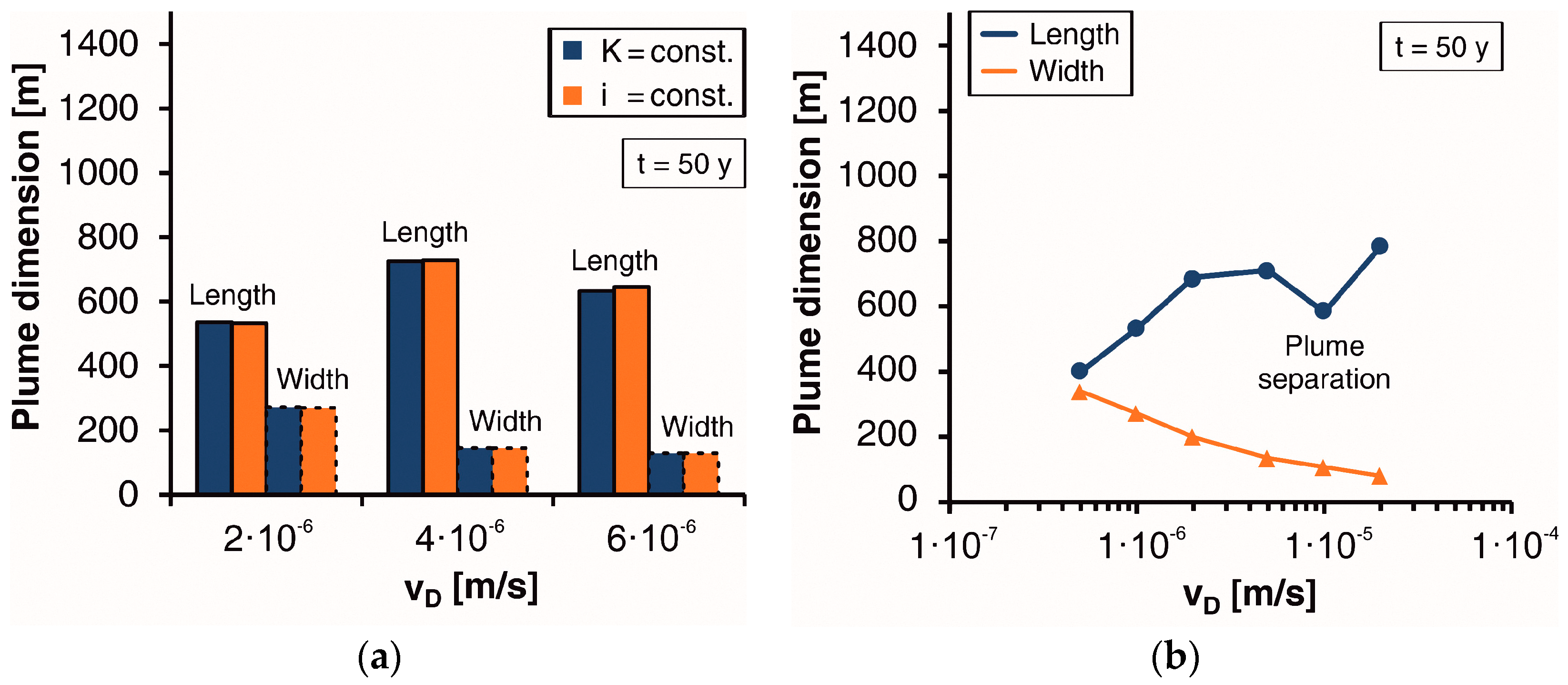
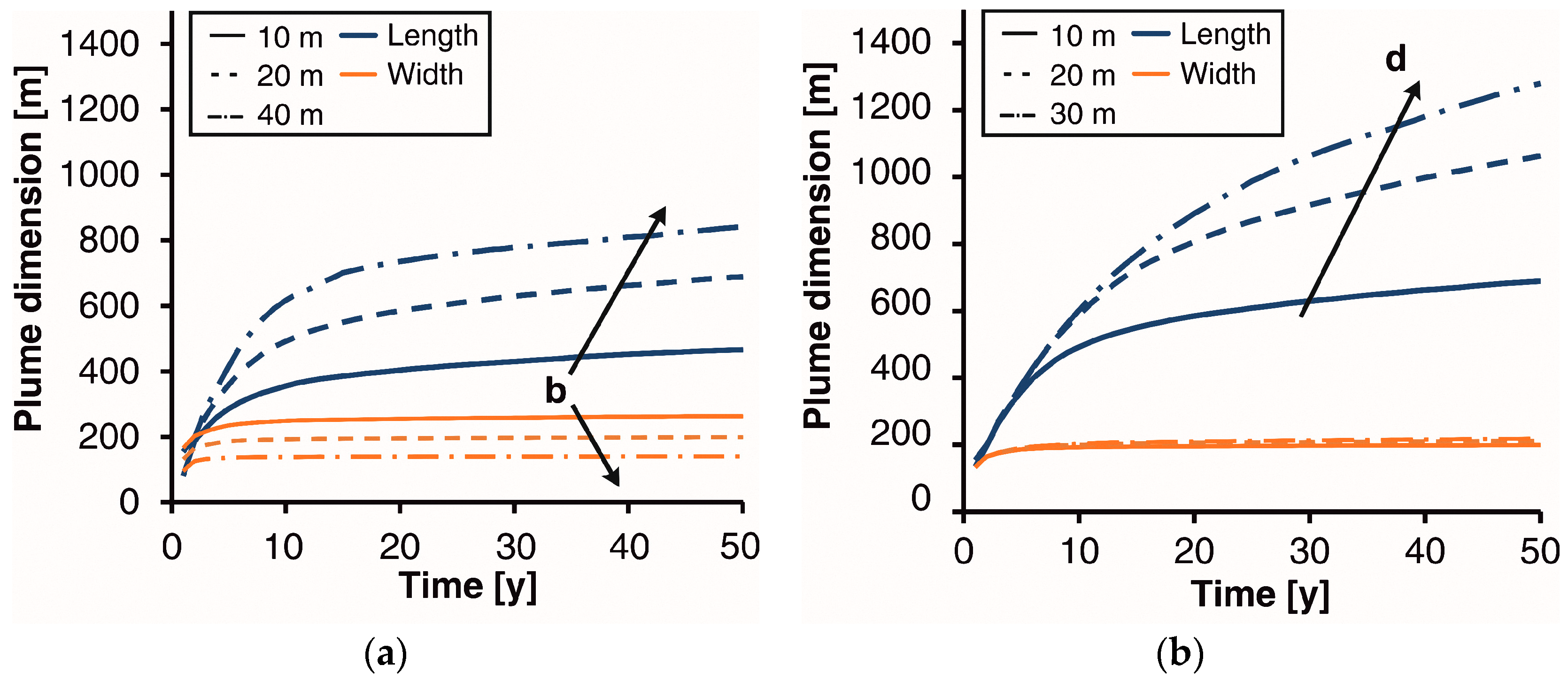
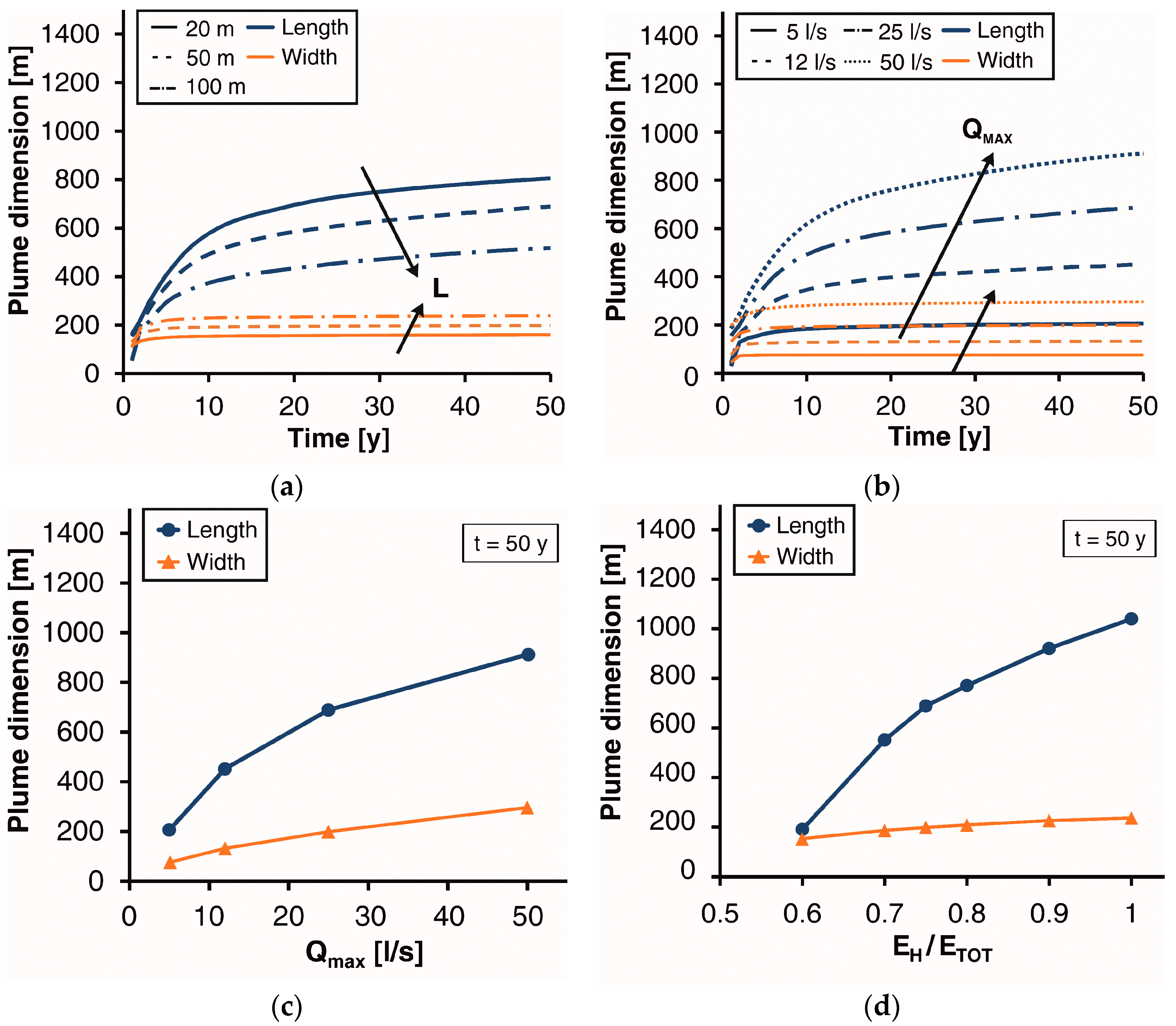
3. Results and Discussion

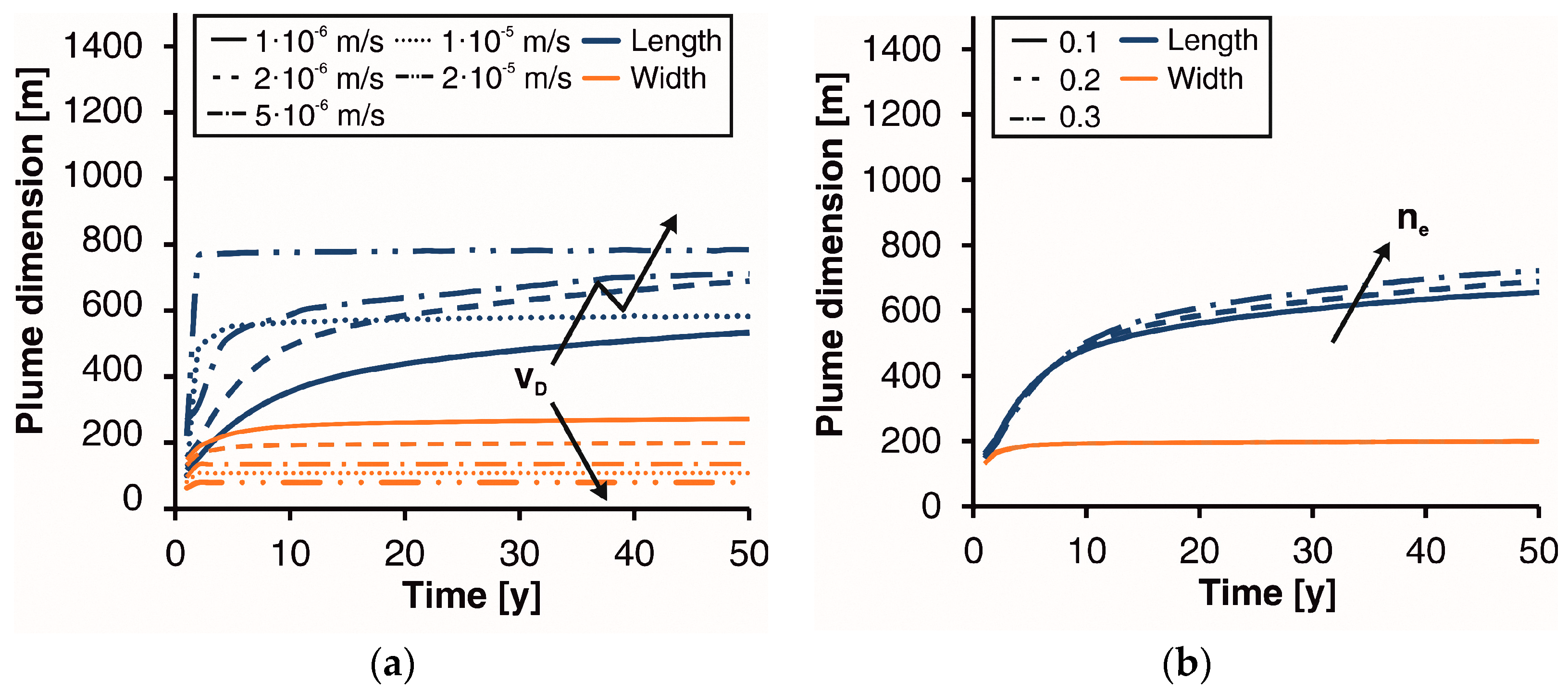
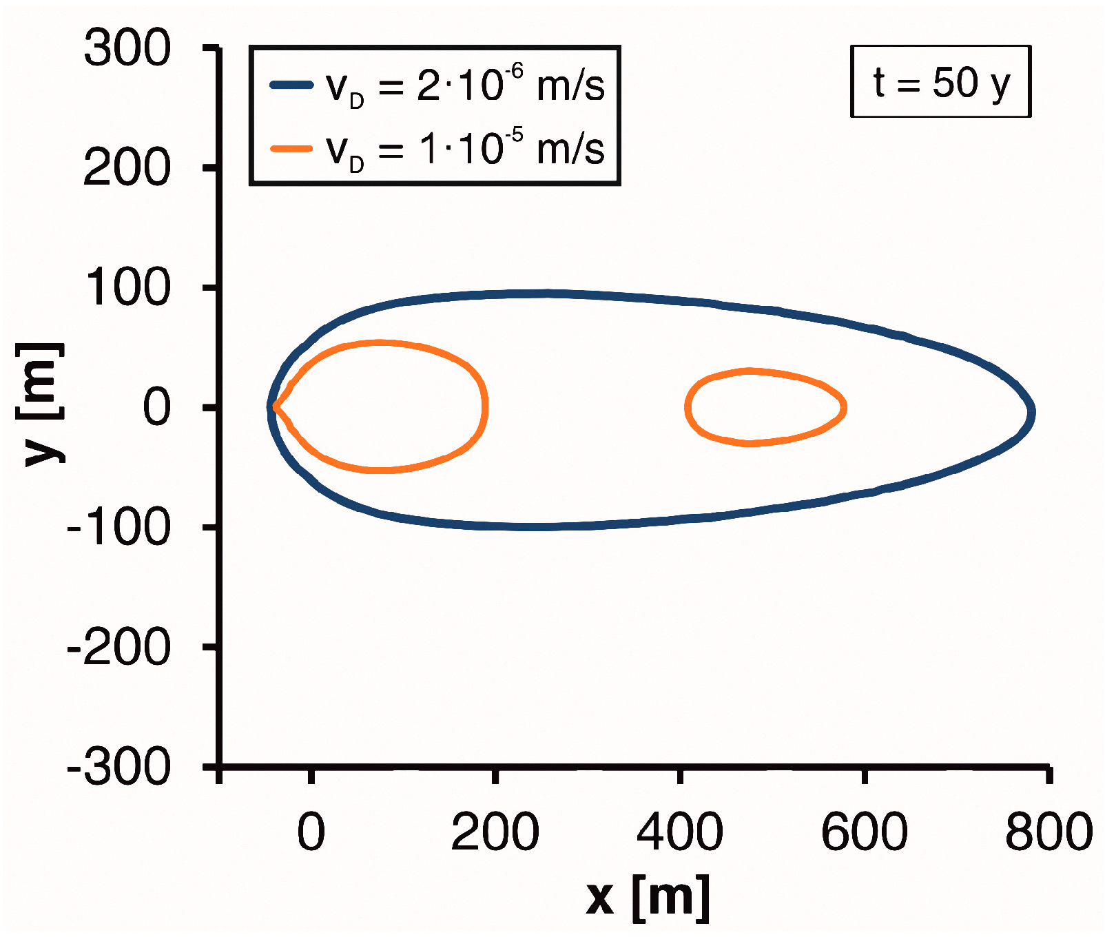
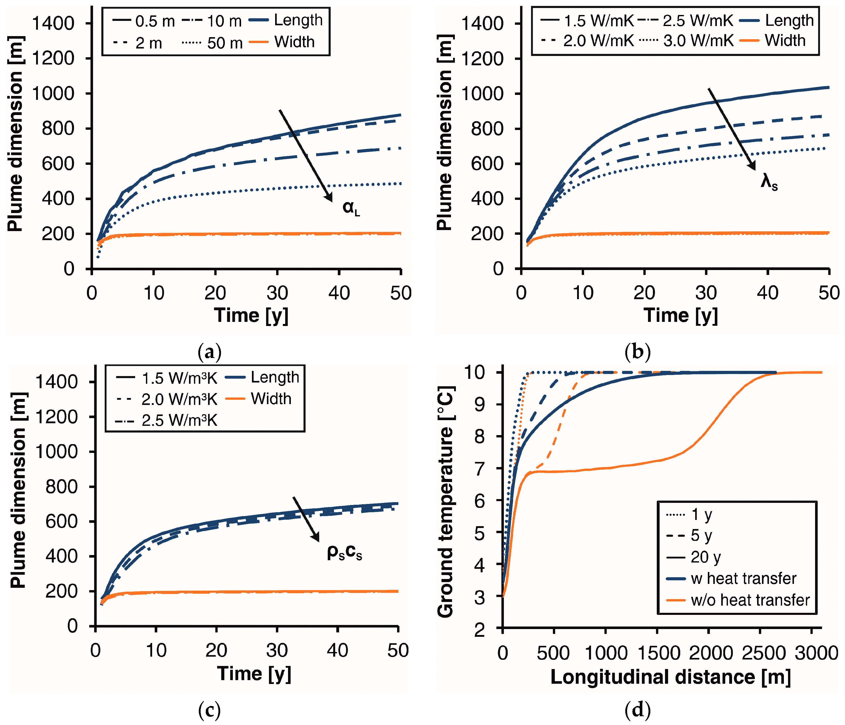
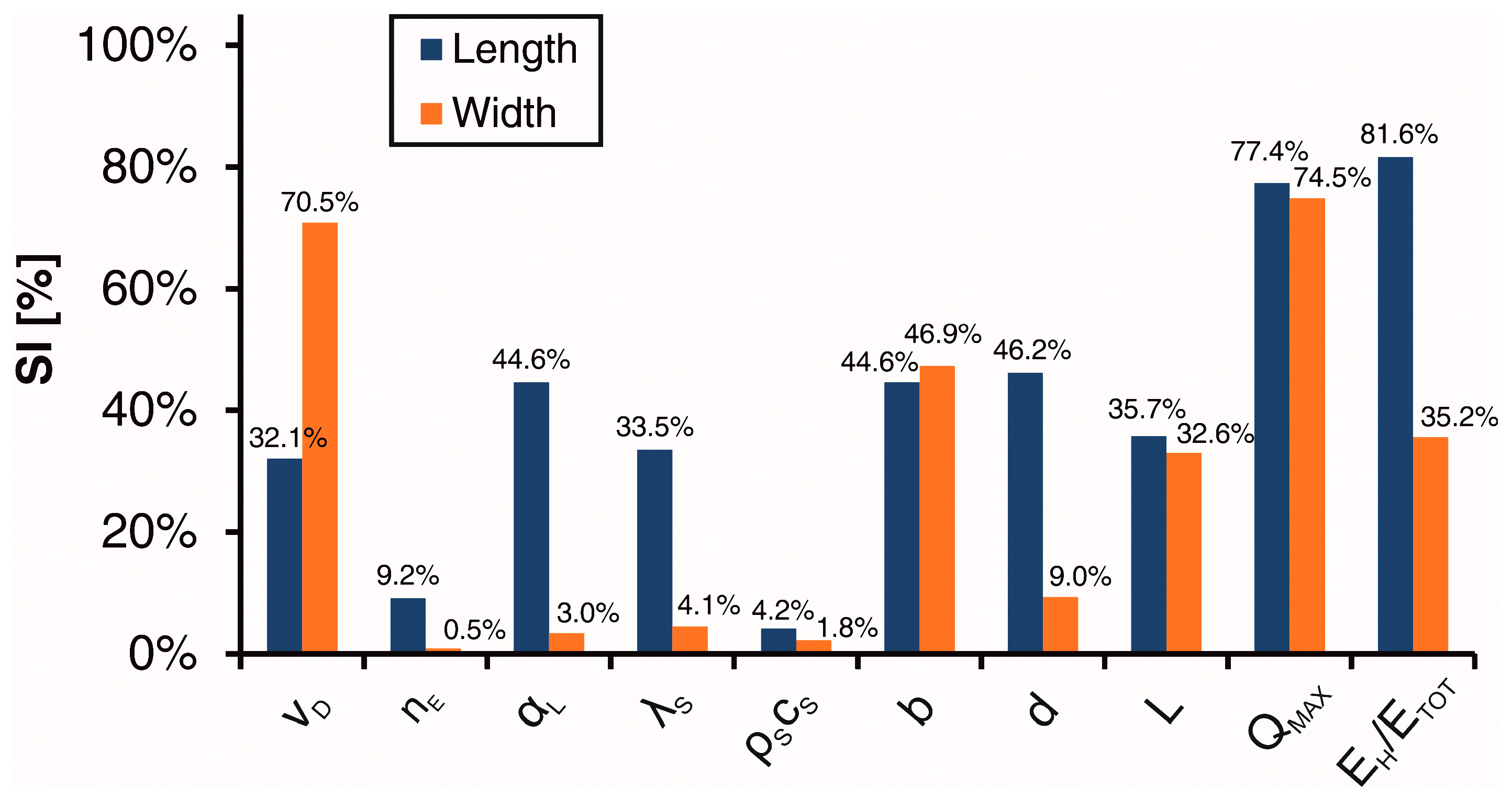
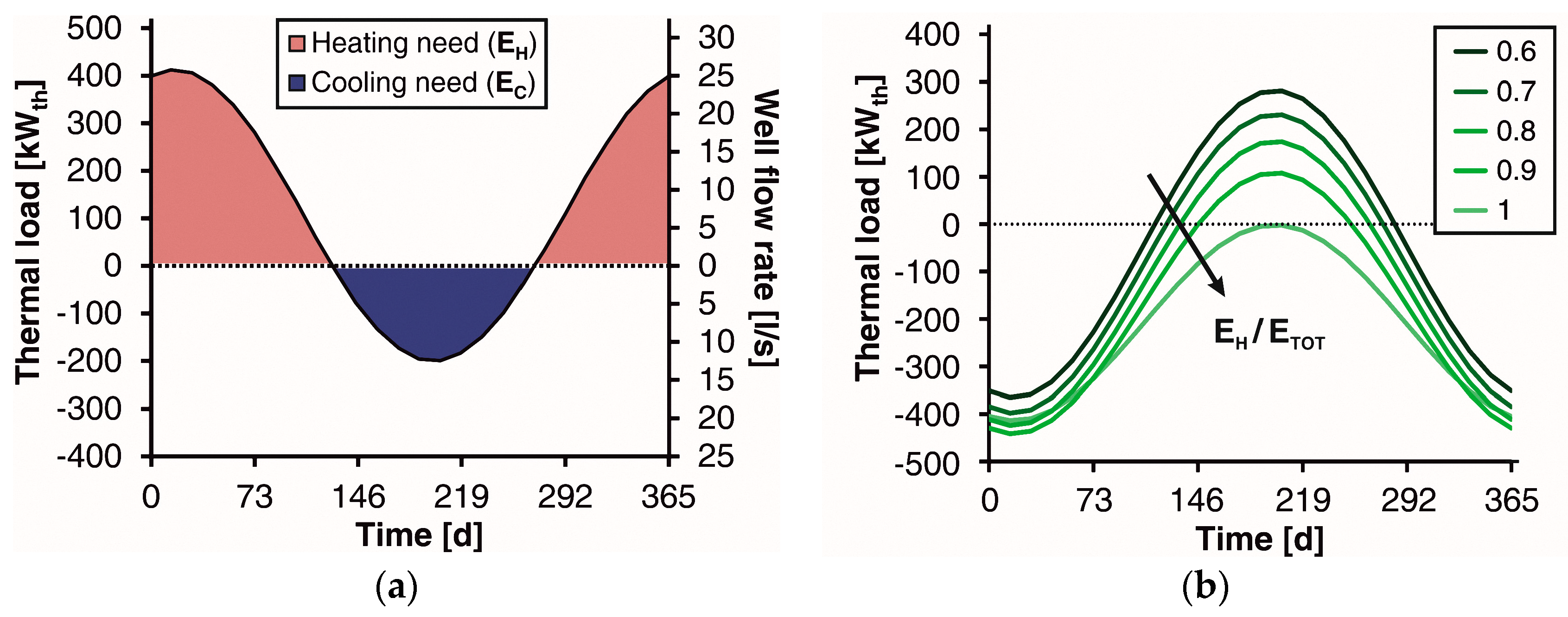
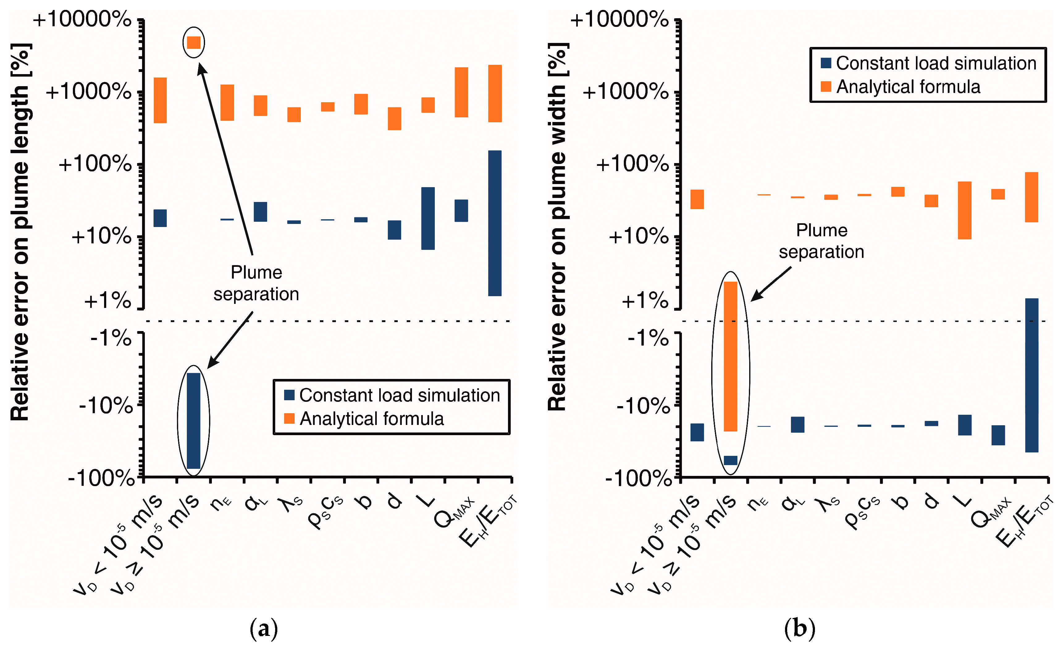
3.1. Sensitivity Analysis

The results of the sensitivity analysis aim at identifying the parameters that have the strongest influence on the dimensions of a thermal plume. Starting from the hydrodynamic parameters, hydraulic conductivity ($K$) and hydraulic gradient ($i$), we observe that plume propagation only depends on the thermal velocity ($v_{th}=Ki/\left(n_e{R}_{th}\right),$ from Equations (3), (6) and (7)). Conversely, the plume size is almost insensitive to the single values of $K$ and $i$ (Figure 4a). Indeed, the hydraulic conductivity only influences the spatial distribution of the hydraulic head and, consequently, of the flow field close to the abstraction and injection wells. This effect is negligible far downstream of the well doublet.

Based on this result, the successive parametric sweep focused on variations of the Darcy velocity $v_D$. As expected, higher values of $v_D$ lead to a considerable increase in the plume length and a dramatic decrease in its width (Figure 4b). A one order of magnitude increase in the regional groundwater velocity reduces the width of the thermal plume by more than 60%.

The plume extension also reaches a stationary value in a shorter time when the Darcy velocity increases (Figure 5a), with a trend similar to the Moving Infinite Line Source analytical solution [43]. It is also interesting to note that, as the regional groundwater flow velocity increases beyond a certain value ($v_D=1\times {10}^{-5}\mathrm{m}/\mathrm{s}$), the plume length suddenly drops (Figure 4b and Figure 5a). If the Darcy velocity value increases further, the plume length starts to increase again. Indeed, if the groundwater velocity is high enough, the thermal plumes produced in each heating and cooling season are separated into two or more smaller plumes which travel downgradient, while cold and warm plumes are merged at lower velocities (Figure 6). In this case, the farthest plume was considered for length determination.

The drop of the plume length at high groundwater velocities can be explained by the fact that the separation of cold and hot plumes results in a more efficient heat exchange with the neighbouring layers (the vadose zone and aquitard), and, hence, the total length of the plume is reduced. Our results confirm the conclusion drawn in previous studies that the hydrodynamic parameters of the aquifer have a very strong influence on thermal plume size [44,45,46,47]. Hydraulic conductivity is the parameter most subject to uncertainties, depending on the method of determination [12,48]; therefore, it strongly affects the thermal impact quantification of GWHPs.

Unlike the Darcy velocity, the effective porosity has little effect on the plume length, exerted only in the long term (Figure 5b), and does not affect the plume width. Understanding how effective porosity affects the plume dimensions is not straightforward, since different variations of heat transport parameters occur as $n_e$ varies. When the effective porosity increases, the thermal capacity of the porous medium $\rho c$ generally increases, since the thermal capacity is usually higher for groundwater than for the solid phase (${\rho }_w{c}_w>{\rho }_s{c}_s$).

An increment of $n_e$ results in a decrease in the effective velocity of groundwater ($v_e$); on the other hand, the thermal retardation factor ($R_{th}$) also decreases, according to Equation (7). This eventually results in a slight decrease in the thermal velocity $v_{th}=v_e/R_{th}$. Therefore, if we consider only advection, a slight decrease in the plume length would be expected. However, an increase in the effective porosity also causes a reduction of the total thermal conductivity of the porous medium (Equation (4)), since groundwater is usually less conductive than the solid phase (${\lambda }_{\mathrm{w}}<{\lambda }_s$), and this makes the plume length increase, as explained later in this section. These contrasting effects are reflected in plume propagation. As long as the plume is expanding in the aquifer and the propagation towards the unsaturated layers is negligible (i.e., at the onset of GWHP operation), the length of the thermally affected zone diminishes as the effective porosity increases. On the other hand, as the plume also starts to expand in the unsaturated layers, the reduction of the thermal conductivity of the porous medium above and below the saturated zone due to a higher porosity value results in a slight long-term increase in the thermal plume length (Figure 5b).

Thermal dispersivity is one of the most influential aquifer properties for the propagation of thermal plumes; however, the scarcity of information and reliable experimental data available on this topic causes significant design issues [49,50,51]. As is evident from Figure 7a, the thermal dispersivity has a considerable effect on plume length, while its effect on plume width is negligible, especially for low dispersivity values.

When the value of dispersivity increases, energy dissipation in the aquifer increases, so the plume propagates slower, along the groundwater flow direction. Furthermore, longitudinal thermal dispersivities below 2 m do not sensibly influence the extension of the plume: we observe a negligible difference between ${\alpha }_L=0.5\mathrm{m}$ and ${\alpha }_L=2\mathrm{m}$. This is an interesting finding for addressing the numerical modelling issue of oscillatory results, which arise when null or very low dispersivity values are adopted in the presence of strong advection [34]. Usually, in these cases, upwinding schemes are used to introduce a numerical dispersion, thus avoiding the oscillation of model results, but also altering them [34]. It is therefore possible to avoid using upwinding schemes by assigning thermal dispersivities of ${\alpha }_L<2\mathrm{m}$ and ${\alpha }_T<0.2\mathrm{m}$; this prevents both oscillatory results and the underestimation of the thermal impact on the aquifer. Values of dispersivity higher than 2 m should be set carefully, since they could lead to a strong reduction of the estimated plume length (e.g., −45% for ${\alpha }_L=50\mathrm{m}$ relative to ${\alpha }_L=2\mathrm{m}$), as shown in Figure 7a. Notably, variations in the longitudinal and transverse dispersivity do not affect the maximum plume width, which mainly depends on the hydrodynamic aquifer properties.

A few numerical simulation studies of open-loop plants in the long-term (in the order of tens of years) have been published. In previous studies, limited to the saturated layer [44] and usually considering a time span up to one year [32,44], the heat conduction mechanism is negligible compared to advection and dispersion. However, when a sufficiently long time is considered, the conductive propagation of heat in the ground also involves the vadose zone above the aquifer and the underlying layers [52].

Figure 7d depicts the effect of such a mechanism on the longitudinal temperature distribution, comparing the assumptions of a no-flux boundary condition (second kind) applied to the ground surface and of the aforementioned reference temperature (third kind BC). The effect of heat exchange with neighbouring layers gets stronger over time (Figure 7b,d) and is negligible in the short term; this explains why previous studies, which considered short operating periods (less than one year [32,44,46]), concluded that heat conduction is negligible in GWHPs.

Conversely, the plume width is mainly affected by the hydrodynamic parameters of the aquifer, while the heat exchange has a negligible effect.

The volumetric heat capacity of the solid matrix has a minor influence on the plume size in the long-term, as shown in Figure 7c. Both the plume width and length slightly decrease as the thermal capacity of the porous medium ($\rho c$) increases. This is due to the capability of a portion of the aquifer to store a greater amount of heat, given the same thermal alteration.

Long-term propagation of thermal plumes is also influenced by the thickness of the saturated and vadose zones, which both play a substantial role in the expansion of the thermal plume. As the saturated thickness increases (Figure 8a), the plume takes longer to reach the top of the aquifer and exchange heat with the unsaturated zone. Hence, the conductive exchange with neighbouring layers occurs later and heat remains confined for a longer period of time in the aquifer. This implies that the plume propagates considerably further along the groundwater flow direction, as confirmed by the analytical solutions of a 2D plane-symmetric transient heat transport problem reported by Tan et al. [53].

On the other hand, a higher saturated thickness ($b$) leads to larger aquifer transmissivity, which reduces the width of the plume. Therefore, within the range of saturated thicknesses commonly found in shallow alluvial aquifers (where most of the GWHPs are installed), plume size can vary substantially in the long term.

Similarly, an increase in the unsaturated thickness (d) above the aquifer causes a significant increase in the plume length, while the plume width is insensitive to the depth of the saturated zone (Figure 8b). Indeed, heat transport across the unsaturated layers towards the atmosphere is conductive, and a thicker vadose zone has a higher thermal resistance, which limits this heat transfer mechanism. Figure 8b shows that the effect of vadose zone thickness is visible as the thermal alteration approaches the ground surface. For example, after five years, the plume length curve for $d=10\mathrm{m}$ starts to diverge from the others, and the same occurs after 10 years for the curve with $d=20\mathrm{m}$. This study, therefore, confirms the importance of depth to water table and aquifer thickness on the migration of the thermal plume, as was previously reported [11,19].

To conclude the sensitivity analysis, some plant settings also have an appraisable influence on the propagation of thermal plumes in GWHPs.

The thermal alteration at the injection well depends on the temperature of the re-injected water, which in turn strongly depends on the distance $L$ between the injection and abstraction wells. As shown in Figure 9a, an increase in the distance $L$ results in a decrease in the plume length and an increase in its width. This is due to a reduction of the recycled flow rate (see Equations (15) and (16)), which results in a reduction of the thermal alteration at the reinjection well (which influences the length of the plume), and an increase in the flow rate released downstream of the well doublet ($Q_{pl}$), thus increasing the plume width (see Equation (14)). For the considered plant configuration, no thermal recycling occurs when the injection well is located 100 m downstream of the abstraction well: hence, no variations in the plume dimensions are expected over this value of $L$.

The injected-water flow rate and, therefore, the thermal power exchanged with the ground, has a very strong influence on thermal plume propagation (Figure 9d). The plume length has a roughly logarithmic correlation with the flow rate, and an increase in $Q_{max}$ by a factor of ten results in a fourfold increase in the plume length. On the other hand, the width of the thermally affected area increases almost linearly with the injected flow rate (Figure 9c), as expected from Equation (14). The thermal alteration induced downstream of the injection well during each heating season interacts with the plume generated during the previous cooling season, determining the temperature distribution in the ground. For this reason, keeping the same total heat exchanged ($E_{TOT}=E_H+E_C$) and varying the proportion between the heating ($E_H$) and cooling ($E_C$) demands results in different thermal plume dimensions. As expected, the higher the ratio $E_H/E_{TOT}$, the longer and the wider the cold thermal plume originated by the well doublet (Figure 9d).

Finally, the relative importance of the analysed parameters for thermal plume size after 50 years of plant operation was assessed by means of the Sensitivity Index described by Equation (11). Among the hydrogeological and thermal parameters of the ground, the Darcy velocity $v_D$ is the most influential for plume propagation, both in the longitudinal and the transversal direction (Figure 10). A strong impact on the plume length is also exerted by the dispersivity ${\alpha }_L$ and the thermal conductivity of the solid matrix ${\lambda }_s$, while the porosity $n_e$ and the volumetric heat capacity of the solid matrix ${\rho }_s{c}_s$ have a negligible effect on thermal plume size. Strong variations in the plume length and width were observed while varying geometry parameters, such as the aquifer thickness $b$ and the well spacing $L$, whereas the depth to the water table $d$ is only relevant for plume length. The most important parameter for plume propagation in the long term is the injected water flow rate $Q_{max}$, followed by the ratio of the yearly heating demand over the total demand of the heat pump $E_H/E_{TOT}.$

Detailed results of this parametric study for plume length and width are reported in Tables S1 and S2 of the Supplementary Materials.

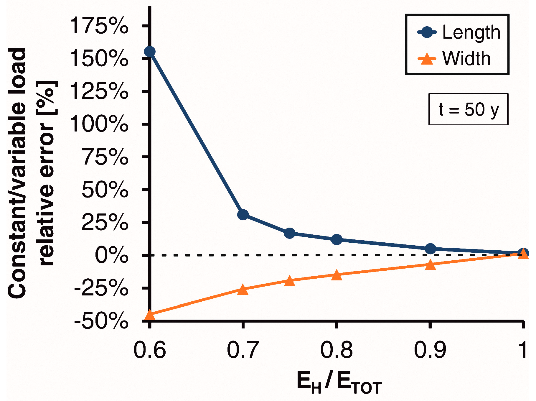
3.2. Comparison with Simplified Models

Transient numerical models are the most precise and rigorous tool for the simulation of the subsurface thermal alteration induced by a GWHP. However, the expense and the time required to perform such simulations are usually very large. Two alternative simplified methods were therefore assessed: numerical simulation with a constant thermal load (equal to the yearly average value, as from Equation (12)) and analytical formulae available for thermal plume length and width evaluation (Equations (13) and (14)) [22]. By imposing a constant thermal load, the computational time for the simulations can be reduced from several hours to a few minutes. Analytical formulae allow fast and inexpensive evaluations of the thermal impact of GWHPs, although they neglect thermal dispersion and conduction.

We used these two approaches to calculate plume length and width at time $t=50\mathrm{years}$, comparing the results with those of the numerical model reported in the previous paragraph in order to assess whether the approximations introduced by these methods are acceptable or not. As shown in Figure 11, simulations performed with a constant thermal load introduce an error in the values of both the plume length and width.

A remarkable result is that, for heating-only systems (i.e., $E_H/E_{TOT}=1$), the plume length is practically the same but, as the heating-cooling imbalance of the thermal load diminishes, the discrepancy increases (Figure 12) by up to about 30% for $E_H/E_{TOT}=70\%$ (which is a fairly acceptable error). As the thermal load approaches the perfect balance between heating and cooling, i.e., $E_H/E_{TOT}=0.5$, the error introduced by this approximation rapidly increases to unacceptable levels.

The yearly averaged load usually leads to an overestimation of the plume length, thus proving a conservative approach, but also to an underestimation of the plume width (Figure 11b). This is due to the fact that the effect of peak flow-rates on the width of the injection well release front is not considered. The tested analytical formula largely overestimates the long-term plume length (Figure 11a), since the advective model described by Equation (13) neglects thermal dispersion and conduction. On the other hand, the plume width can conservatively be estimated with Equation (14), with an acceptable overestimation of 30–60%. Underestimation of the plume width occurs only for the highest considered value of $v_D(2\times {10}^{-5}\mathrm{m}/\mathrm{s}$), because of the plume separation effect and the increased heat dispersion. Hence, the equations proposed by Banks ([22], from Equation (13) to (16)) provide a good and conservative estimation of the plume width, while they cannot be used to assess the longitudinal extension of the thermally affected area.

For detailed results of the methods comparison study, for simulations at 10 years and 50 years, we refer the reader to Tables S1 and S2 of the Supplementary Materials.

4. Conclusions

Assessing the long-term subsurface thermal impact of open-loop geothermal systems is of crucial importance for their design and their proper spatial planning. Various numerical models and analytical solutions can be used to estimate the thermal plume produced by a GWHP, each characterized by different costs, degrees of complexity, and precision.

This work presents a parametric study through numerical flow and heat transport simulations carried out to identify key parameters and compare their relative influence within their typical ranges of variation. Moreover, simplified numerical modelling with a constant thermal load and analytical solutions for 2D plume propagation in an aquifer were investigated to quantify the discrepancy compared to transient numerical modelling.

Among the hydraulic and thermal subsurface parameters, the most influential for both plume length and width is the Darcy velocity ($v_D$), i.e., the product of hydraulic conductivity ($K$) and gradient ($i$). In this light, it is very important to determine the hydraulic conductivity with reliable in-situ tests, in order to perform realistic simulations and avoid major errors in plume size estimations.

The thermal properties of the ground affect the plume length but have a negligible influence on its width. In particular, thermal conductivity ($\lambda$) and dispersivity ($\alpha$) of the ground play an important role in the long-term, while variations of heat capacity ($\rho c$) have minor effects on plume size.

Depth to water table ($d$) and aquifer thickness ($b$) are also key factors in the propagation of thermal plumes, thus confirming the necessity of a 3D modelling geometry. Plume length dramatically increases with the thickness of the saturated and unsaturated zones, as thermal exchange with air is reduced, and propagation of the thermal plume is confined to the saturated zone. On the other hand, an increase in the saturated thickness results in higher transmissivity and, consequently, in a reduction of the plume width with an almost linear inverse trend.

The distance between abstraction and injection wells ($L$) noticeably influences the width of the thermal plume, while its impact on its longitudinal extension is lower, though not negligible.

Regarding thermal loads, a logarithmic increase in the plume length with the abstracted/injected flow rate (and consequently with the thermal power) is observed, while the correlation is almost linear for the plume width. The balancing of the heating and cooling demand of the building sensibly affects the size of the thermal plume, which reaches its maximum for a fully heating-dominated (or cooling-dominated) demand and its minimum for a perfectly balanced load.

The assessment of the thermal plume adopting a constant thermal load (equal to its yearly average) is not reliable at high groundwater velocities, due to the separation of plumes originated during heating and cooling seasons. In such cases, a simulation with a time-varying thermal load is required.

On the other hand, for heating or cooling-dominated loads, constant load simulations provide a good approximation of the thermal plume lengths. In this way, the computational time is drastically reduced, and simpler and cheaper software can be used. For balanced or slightly unbalanced thermal loads, however, the length of the thermal plume is largely overestimated using the constant load approach.

Finally, analytical formulae for 2D advective propagation provided by Banks [22] can be used to quickly assess the width of thermal plumes, while they provide unrealistically high estimates of the plume length.

We provide useful insights for the evaluation of the thermal impact of GWHPs on aquifers, and hence for their planning in densely inhabited areas. The key parameters are identified, along with the error margins deriving from a poor characterisation of the site.

The effects of simplifying assumptions, such as using the yearly average of the thermal load or adopting available analytical solutions, are also analysed, thus defining under what conditions such methods can be used with acceptable accuracy.

References

1. Ouzzane, M.; Eslami-Nejad, P.; Badache, M.; Aidoun, Z. New correlations for the prediction of the undisturbed ground temperature. Geothermics 2015, 53, 379–384. [Google Scholar] [CrossRef]
2. Omer, A.M. Ground-source heat pumps systems and applications. Renew. Sustain. Energy Rev. 2008, 12, 344–371. [Google Scholar] [CrossRef]
3. Bayer, P.; Saner, D.; Bolay, S.; Rybach, L.; Blum, P. Greenhouse gas emission savings of ground source heat pump systems in Europe: A review. Renew. Sustain. Energy Rev. 2012, 16, 1256–1267. [Google Scholar] [CrossRef]
4. Chung, J.T.; Choi, J.M. Design and performance study of the ground-coupled heat pump system with an operating parameter. Renew. Energy 2012, 42, 118–124. [Google Scholar] [CrossRef]
5. Dehkordi, S.E.; Schincariol, R. Effect of thermal-hydrogeological and borehole heat exchanger properties on performance and impact of vertical closed-loop geothermal heat pump systems. Hydrogeol. J. 2014, 22, 189–203. [Google Scholar] [CrossRef]
6. Casasso, A.; Sethi, R. G.POT: A quantitative method for the assessment and mapping of the shallow geothermal potential. Energy 2016, 106, 765–773. [Google Scholar] [CrossRef]
7. Casasso, A.; Sethi, R. Sensitivity Analysis on the Performance of a Ground Source Heat Pump Equipped with a Double U-pipe Borehole Heat Exchanger. Energy Procedia 2014, 59, 301–308. [Google Scholar] [CrossRef]
8. Casasso, A.; Sethi, R. Territorial Analysis for the Implementation of Geothermal Heat Pumps in the Province of Cuneo (NW Italy). Energy Procedia 2015, 78, 1159–1164. [Google Scholar] [CrossRef]
9. Casasso, A.; Sethi, R. Modelling thermal recycling occurring in groundwater heat pumps (GWHPs). Renew. Energy 2015, 77, 86–93. [Google Scholar] [CrossRef]
10. Galgaro, A.; Cultrera, M. Thermal short circuit on groundwater heat pump. Appl. Therm. Eng. 2013, 57, 107–115. [Google Scholar] [CrossRef]
11. Stauffer, F.; Bayer, P.; Blum, P.; Molina-Giraldo, N.; Kinzelbach, W. Thermal Use of Shallow Groundwater; CRC Press—Taylor and Francis Group: Boca Raton, FL, USA, 2013; p. 250. [Google Scholar]
12. Di Molfetta, A.; Sethi, R. Ingegneria Degli Acquiferi; Springer: Berlin, Germany, 2012; p. 370. [Google Scholar]
13. Ampofo, F.; Maidment, G.G.; Missenden, J.F. Review of groundwater cooling systems in London. Appl. Therm. Eng. 2006, 26, 2055–2062. [Google Scholar] [CrossRef]
14. Beretta, G.P.; Coppola, G.; Pona, L.D. Solute and heat transport in groundwater similarity: Model application of a high capacity open-loop heat pump. Geothermics 2014, 51, 63–70. [Google Scholar] [CrossRef]
15. De Santoli, L.; Mancini, F.; Rossetti, S. The energy sustainability of Palazzo Italia at EXPO 2015: Analysis of an nZEB building. Energy Build. 2014, 82, 534–539. [Google Scholar] [CrossRef]
16. Piemonte, C.; Porro, A. Palazzo Lombardia—Geothermal Heat Pump Capacity World Record for a Single Building Conditioning. In Proceedings of the European Geothermal Conference, Pisa, Italy, 3–7 June 2013; pp. 1–4. [Google Scholar]
17. Bouwer, H. Artificial recharge of groundwater: Hydrogeology and engineering. Hydrogeol. J. 2002, 10, 121–142. [Google Scholar] [CrossRef]
18. Banks, D. Thermogeological assessment of open-loop well-doublet schemes: A review and synthesis of analytical approaches. Hydrogeol. J. 2009, 17, 1149–1155. [Google Scholar] [CrossRef]
19. Banks, D. An Introduction to Thermogeology: Ground Source Heating and Cooling; John Wiley & Sons: Hoboken, NJ, USA, 2012; p. 526. [Google Scholar]
20. Gringarten, A.C.; Sauty, J.P. A theoretical study of heat extraction from aquifers with uniform regional flow. J. Geophys. Res. 1975, 80, 4956–4962. [Google Scholar] [CrossRef]
21. Lippmann, M.J.; Tsang, C.F. Ground-Water Use for Cooling: Associated Aquifer Temperature Changes. Ground Water 1980, 18, 452–458. [Google Scholar] [CrossRef]
22. Banks, D. The application of analytical solutions to the thermal plume from a well doublet ground source heating or cooling scheme. Q. J. Eng. Geol. Hydrogeol. 2011, 44, 191–197. [Google Scholar] [CrossRef]
23. Shan, C. An analytical solution for the capture zone of two arbitrarily located wells. J. Hydrol. 1999, 222, 123–128. [Google Scholar] [CrossRef]
24. Luo, J.; Kitanidis, P.K. Fluid residence times within a recirculation zone created by an extraction–injection well pair. J. Hydrol. 2004, 295, 149–162. [Google Scholar] [CrossRef]
25. Milnes, E.; Perrochet, P. Assessing the impact of thermal feedback and recycling in open-loop groundwater heat pump (GWHP) systems: A complementary design tool. Hydrogeol. J. 2013, 21, 505–514. [Google Scholar] [CrossRef]
26. Bridger, D.W.; Allen, D.M. Heat transport simulations in a heterogeneous aquifer used for aquifer thermal energy storage (ATES). Can. Geotech. J. 2010, 47, 96–115. [Google Scholar] [CrossRef]
27. Bridger, D.W.; Allen, D.M. Influence of geologic layering on heat transport and storage in an aquifer thermal energy storage system. Hydrogeol. J. 2014, 22, 233–250. [Google Scholar] [CrossRef]
28. Nam, Y.; Ooka, R. Numerical simulation of ground heat and water transfer for groundwater heat pump system based on real-scale experiment. Energy Build. 2010, 42, 69–75. [Google Scholar] [CrossRef]
29. Ferguson, G.; Woodbury, A.D. Observed thermal pollution and post-development simulations of low-temperature geothermal systems in Winnipeg, Canada. Hydrogeol. J. 2006, 14, 1206–1215. [Google Scholar] [CrossRef]
30. Fry, V.A. Lessons from London: Regulation of open-loop ground source heat pumps in central London. Q. J. Eng. Geol. Hydrogeol. 2009, 42, 325–334. [Google Scholar] [CrossRef]
31. García-Gil, A.; Vázquez-Suñe, E.; Schneider, E.G.; Sánchez-Navarro, J.Á.; Mateo-Lázaro, J. The thermal consequences of river-level variations in an urban groundwater body highly affected by groundwater heat pumps. Sci. Total Environ. 2014, 485–486, 575–587. [Google Scholar]
32. Lo Russo, S.; Gnavi, L.; Roccia, E.; Taddia, G.; Verda, V. Groundwater Heat Pump (GWHP) system modeling and Thermal Affected Zone (TAZ) prediction reliability: Influence of temporal variations in flow discharge and injection temperature. Geothermics 2014, 51, 103–112. [Google Scholar] [CrossRef]
33. Poppei, J.; Mayer, G.; Schwarz, R. Groundwater Energy Designer (GED)—Computergestütztes Auslegungstool zur Wärme und Kältenutzung von Grundwasser [Computer Assisted Design Tool for the Use of Heat and Cold from Groundwater]; Bundesamt für Energie BFE: Ittigen, Switzerland, 2006; pp. 1–71. [Google Scholar]
34. Diersch, H.J.G. FEFLOW. Finite Element Modeling of Flow, Mass and Heat Transport in Porous and Fractured Media; Springer: Berlin/Heidelberg, Germany, 2014; p. 996. [Google Scholar]
35. Epting, J.; Huggenberger, P. Unraveling the heat island effect observed in urban groundwater bodies—Definition of a potential natural state. J. Hydrol. 2013, 501, 193–204. [Google Scholar] [CrossRef]
36. Kim, K.Y.; Chon, C.M.; Park, K.H.; Park, Y.S.; Woo, N.C. Multi-depth monitoring of electrical conductivity and temperature of groundwater at a multilayered coastal aquifer: Jeju Island, Korea. Hydrol. Process. 2008, 22, 3724–3733. [Google Scholar] [CrossRef]
37. Lee, J.-Y. Characteristics of ground and groundwater temperatures in a metropolitan city, Korea: Considerations for geothermal heat pumps. Geosci. J. 2006, 10, 165–175. [Google Scholar] [CrossRef]
38. Lee, J.-Y.; Hahn, J.-S. Characterization of groundwater temperature obtained from the Korean national groundwater monitoring stations: Implications for heat pumps. J. Hydrol. 2006, 329, 514–526. [Google Scholar] [CrossRef]
39. Bense, V.; Kooi, H. Temporal and spatial variations of shallow subsurface temperature as a record of lateral variations in groundwater flow. J. Geophys. Res. Solid Earth 2004, 109, B4. [Google Scholar] [CrossRef]
40. Heiselberg, P.; Brohus, H.; Hesselholt, A.; Rasmussen, H.; Seinre, E.; Thomas, S. Application of sensitivity analysis in design of sustainable buildings. Renew. Energy 2009, 34, 2030–2036. [Google Scholar] [CrossRef]
41. De Marsily, G. Quantitative Hydrogeology; Academic Press: San Diego, CA, USA, 1986; p. 464. [Google Scholar]
42. Schulze-Makuch, D. Longitudinal dispersivity data and implications for scaling behavior. Ground Water 2005, 43, 443–456. [Google Scholar] [CrossRef] [PubMed]
43. Molina-Giraldo, N.; Blum, P.; Zhu, K.; Bayer, P.; Fang, Z. A moving finite line source model to simulate borehole heat exchangers with groundwater advection. Int. J. Therm. Sci. 2011, 50, 2506–2513. [Google Scholar] [CrossRef]
44. Lo Russo, S.; Taddia, G.; Verda, V. Development of the thermally affected zone (TAZ) around a groundwater heat pump (GWHP) system: A sensitivity analysis. Geothermics 2012, 43, 66–74. [Google Scholar] [CrossRef]
45. Böttcher, F. Estimation of Characteristic Heat Flow Current Extents in the North of Münchener Schotterebene; TUM: Munich, Germany, 2014. [Google Scholar]
46. Park, B.-H.; Bae, G.-O.; Lee, K.-K. Importance of thermal dispersivity in designing groundwater heat pump (GWHP) system: Field and numerical study. Renew. Energy 2015, 83, 270–279. [Google Scholar] [CrossRef]
47. Angelotti, A.; Alberti, L.; La Licata, I.; Antelmi, M. Energy performance and thermal impact of a Borehole Heat Exchanger in a sandy aquifer: Influence of the groundwater velocity. Energy Convers. Manag. 2014, 77, 700–708. [Google Scholar] [CrossRef]
48. Butler, J.J., Jr.; Healey, J.M. Relationship between pumping-test and slug-test parameters: Scale effect or artifact? Ground Water 1998, 36, 305–313. [Google Scholar] [CrossRef]
49. Vandenbohede, A.; Lebbe, L. Parameter estimation based on vertical heat transport in the surficial zone. Hydrogeol. J. 2010, 18, 931–943. [Google Scholar] [CrossRef]
50. Gelhar, L.W.; Welty, C.; Rehfeldt, K.R. A critical review of data on field-scale dispersion in aquifers. Water Resour. Res. 1992, 28, 1955–1974. [Google Scholar] [CrossRef]
51. Ferguson, G. Heterogeneity and thermal modeling of ground water. Groundwater 2007, 45, 485–490. [Google Scholar] [CrossRef] [PubMed]
52. Barends, F. Complete solution for transient heat transport in porous media, following Lauwerier. In Proceedings of the SPE Annual Technical Conference and Exhibition, Florence, Italy, 19–22 September 2010. [Google Scholar]
53. Tan, H.; Cheng, X.; Guo, H. Closed Solutions for Transient Heat Transport in Geological Media: New Development, Comparisons, and Validations. Transp. Porous Media 2012, 93, 737–752. [Google Scholar] [CrossRef]
Figure 1. Simplified 2D cross-section of the GWHP plant 3D model in heating mode.
Energies 10 01385 g001
Figure 2. (a) Time series of the yearly-cyclic thermal load (left y-axis) and pumping/injection rates (right y-axis) applied in the well-doublet at default conditions (thick black line) and (b) for the heat-balance sensitivity analysis.
Energies 10 01385 g002
Figure 3. Plume dimensions considered in the sensitivity analysis.
Energies 10 01385 g003
Figure 4. Plume dimensions after a 50 years simulation for different combinations of hydraulic conductivity K and gradient i (a) and for different values of Darcy velocity v D (b); isotherm ∆T = 1 °C.
Energies 10 01385 g004
Figure 5. Time evolution of plume dimensions with Darcy velocity v D (a) and effective porosity n e (b); isotherm ∆T = 1 °C.
Energies 10 01385 g005
Figure 6. Thermal plume shape after a 50 years simulation, for different values of Darcy velocity v D ; isotherm ∆T = 1 °C.
Energies 10 01385 g006
Figure 7. Time evolution of plume dimensions with different values of longitudinal thermal dispersivity α L (a); solid matrix thermal conductivity λ s (b); and thermal capacity ρ s c s (c); longitudinal temperature profile downstream of the reinjection well with and without considering heat exchange with unsaturated layers, for the default simulation and at different times (d); isotherm ∆T = 1 °C.
Energies 10 01385 g007
Figure 8. Time evolution of plume dimensions with different values of aquifer thickness b (a) and vadose zone thickness d (b); isotherm ∆T = 1 °C.
Energies 10 01385 g008
Figure 9. Time evolution of plume dimensions with different values of well spacing L (a) and maximum annual injected flow rate Q m a x (b); plume dimensions after 50 years for different values of maximum annual injected flow rate Q m a x (c) and ratio of energy demand for heating over total demand E H / E T O T (d); isotherm ∆T = 1 °C.
Energies 10 01385 g009
Figure 10. Sensitivity index (SI) values for each parameter of the sensitivity analysis, for plume length and width after 50-year simulations.
Energies 10 01385 g010
Figure 11. Relative error on plume length (a) and width (b), evaluated with a constant thermal load simulation and analytical formulae, compared to a variable thermal load simulation, for the considered range of parameters; isotherm ∆T = 1 °C, t = 50 years.
Energies 10 01385 g011
Figure 12. Relative error on plume dimensions of constant thermal load simulations compared to variable load simulations, with different values of the ratio of heating over total demand E H / E T O T ; isotherm ∆T = 1 °C.
Energies 10 01385 g012