1. Introduction
The effective detection and diagnosis of coal-fired power plant furnace flames is required for the safe operation of power plant boilers. Various methods for flame detection and diagnosis have been reported [
1,
2,
3,
4,
5]. The laser spectroscopy method [
6] has high temporal and spatial resolution, and can be used to measure temperature and to determine the concentrations of many components during the combustion process. However, expensive equipment and complex optical systems are required; therefore, this approach is not easily applied to industrial furnaces. Image processing techniques, based on a tri-chromatic signal of the image and using the two-color method, have been widely used for temperature measurements of furnace flames [
7,
8,
9,
10]. The emission from emitters at two wavelengths is utilized to calculate the temperature and emissivity in image processing techniques. However, the radiation energy of the tri-chromatic signal is not exactly monochromatic and the wavelengths of the tri-chromatic signal may vary between different image acquisition systems [
11]. Additionally, the method fails to detect radical radiation in the flame. A fiber-optic spectrometer system with a simple structure, low data processing requirements, and an ability for gathering additional information may be more useful for flame diagnosis. At the same time, this method can achieve an online detection of temperature and emissivity, as well as radical radiation for certain components, such as CH*, C
2*, Na*, and K*.
Flame spectra are classified depending on the energy distribution of continuous and discontinuous spectra [
12]. For continuous spectra, the emitted or absorbed energy is distributed in a continuous spectrum over a wide wavelength region. The emitted or absorbed energy is mainly concentrated in a narrow band of the spectrum in discontinuous spectra [
13]. Usually, a continuous spectrum represents low-frequency components and the discontinuous emission is characterized by high-frequency components [
14]. The continuous spectrum of a coal-fired flame that is usually applied to calculate temperature provides important information for soot formation [
15]. The existence of discontinuous emission spectra may influence the temperature calculation’s accuracy. On the other hand, supercritical power station boilers are very prone to the coking phenomenon due to very high temperatures and a low ash fusion point in the fuel. The ash fusion point is closely related to the alkali metal content of the fuel. Oleschko et al. [
16] found that alkali metals released during combustion are responsible for the formation of sticky deposits in the boiler. Therefore, accurate measurements of the concentrations of the alkali metal, such as Na* and K*, in a flame are very important for the prevention of deposits that interfere with the proper function of the furnace. The radiation intensity of alkali metals in the furnace flame is not only related to the concentration of the alkali metal vapor but also to the local flame temperature. Building a functional expression between these three parameters can achieve online measurements of the concentration of the alkali metal. However, the continuous and discontinuous spectra are superimposed, but the flame temperature and the actual radiation intensity of the alkali metals depend on continuous and discontinuous spectra. Thus, it is necessary to separate the continuous and discontinuous spectral information from the measured flame spectrum. There are automated and manual methods for separating the discontinuous and continuous spectra in the spectra of coal-fired flames [
17]. Automated methods can automatically estimate a continuous baseline from the measured flame spectra, while manual approaches require operator intervention for the selection of several baseline points. Both methods are highly sensitive to signal parameters such as noise [
13].
An emissivity model is required to calculate temperature and emissivity based on a continuous spectrum. Two popular emissivity models have been applied to coal-fired flames. Most researchers have assumed a coal flame to be a gray body emitter with a constant emissivity [
18,
19,
20]. Hottel and Broughton’s soot emissivity model [
21], which is spectrally dependent, is another popular model for radiating soot particles. Nevertheless, no single existing emissivity model can be used in every situation. In fact, the effective implementation of spectrum technology to measure the temperature in a coal flame is dependent on the kinds of emitters present. Generally, visible radiation from coal flames derived from particles such as coal, char, ash, and soot are generated during coal combustion [
22]. Backstrom et al. [
23] reported that the particle radiation within a flame depended not only on the particle concentration and particle temperature, but also on the type of particles, or more precisely, their radiative properties.
Soot particles with strong absorption and emission characteristics and in relatively small quantities are assumed to dominate the emissions. Soot in a coal flame typically consists of individual particles or agglomerates comprised of between several and thousands of primary particles [
24]. The diameter of individual soot particles is about 20–40 nm, and coal, char, and ash particles are about 2–500 μm [
25]. Therefore, soot particles are significantly smaller than the accompanying coal and char particles and can be optically isolated [
4]. However, the soot cloud generated by the decomposition of volatile substances in a high-temperature environment produces a semi-transparent media with an associated equivalent. At the same time, the small size of soot particles produces a larger total surface area and enhances the radiative heat transfer. Fletcher [
24] concluded that, in the presence of a large radiant surface area, the near-burner flame temperature could be lowered several hundred degrees due to the heat transfer to the surrounding walls. Draper [
22] reported that two models for coal combustion flame were not ideal, but that Hottel and Broughton’s soot emissivity model was more suitable and accurate than Gray’s model for the image processing of flame images near the burner.
A simple manual method for spectral separation is proposed and validated in this study. Hottel and Broughton’s emissivity model is applied to obtain the temperature and emissivity of a furnace flame based on estimated continuous spectra. The influence of the discontinuous emission spectra on the calculation of flame temperature and emissivity is also discussed. Finally, the relationship between the temperature and intensity of an alkali metal is discussed.
2. Measurement Principle
The emissive power distribution of a blackbody for a given wavelength can be represented using Planck’s law [
22]:
where
is the spectral emissive power of a blackbody (W/m
−3),
λ is the wavelength (m),
T is temperature (K), and
and
are called Planck’s first and second radiation constant, respectively. However, particles in a pulverized coal flame do not emit blackbody radiation, and the actual spectral emissive power of a non-blackbody is the emissive power of a blackbody multiplied by the spectral emissivity
that can be expressed as follows:
The emissive power is inadequate to describe the directional dependence of the radiation field, especially inside an absorbing/emitting medium, where photons may not have originated from a surface [
26]. Therefore, a related concept that is very similar to the emissive power is the radiative intensity. The relationship between the intensity of a non-blackbody and its emissive power can be expressed as follows [
26]:
In a widely used method, Hottel and Broughton developed an empirical emissivity model shown in Equation (4) for radiating soot particles [
21].
where
is the spectral emissivity,
K is the absorption coefficient,
L is the thickness of the flame along the line-of-sight (m), and
KL, which can be treated as a whole called the optical thickness [
27], is an empirical parameter that depends on the wavelength in the visible range and can be considered a fixed value of 1.39 [
24]. Substituting Equation (4) and (2) into Equation (3), we can obtain the following relationship between radiation intensity,
KL, and
T.
KL and T are the only unknown parameters in the expression. However, for a spectrometer, the output consists of a radiation signal at multiple wavelengths. Thus, there are additional equations for the radiation intensity, KL, and T, so that the number of equations is greater than the number of unknown parameters. To solve the equations, a nonlinear least squares method is applied for calculating KL and T. The value of KL, which is independent of the wavelength, can then be used in Equation (4) to determine the spectrally dependent .
The measurement principle of temperature and emissivity described above is applied to the continuous spectrum. For the flame emission spectrum, which contains both discontinuous and continuous spectra, it is inappropriate to apply the above measurement principle. Indeed, flame emission spectra can be expressed as the sum of the continuous and discontinuous spectral emissions, as shown in Equation (6) [
15].
The objective is to obtain the continuous flame emission Ec from the measured Ee using a simple method based on polynomial fitting. Subsequently, the discontinuous spectral emissions Ed can be estimated. The procedure of the method is summarized below:
- (i).
The narrow bands corresponding to the discontinuous emissions, such as Na* and K*, are removed from the emitted flame spectrum Ee. The rest of the flame emission spectra can be expressed with Ere.
- (ii).
A fifth-order polynomial fitting is used for Ere. The correlation coefficient R is used to evaluate the fitting results. If R is greater than 0.9999, it indicates that the fitting result is satisfactory. Subsequently, the fitting expression can be obtained for the estimated continuous flame emission.
- (iii).
The wavelengths of the entire spectrum, selected for the calculation of temperature and emissivity, are incorporated into the obtained fitting expression. This allows us to estimate the continuous flame emission over a wide wavelength region.
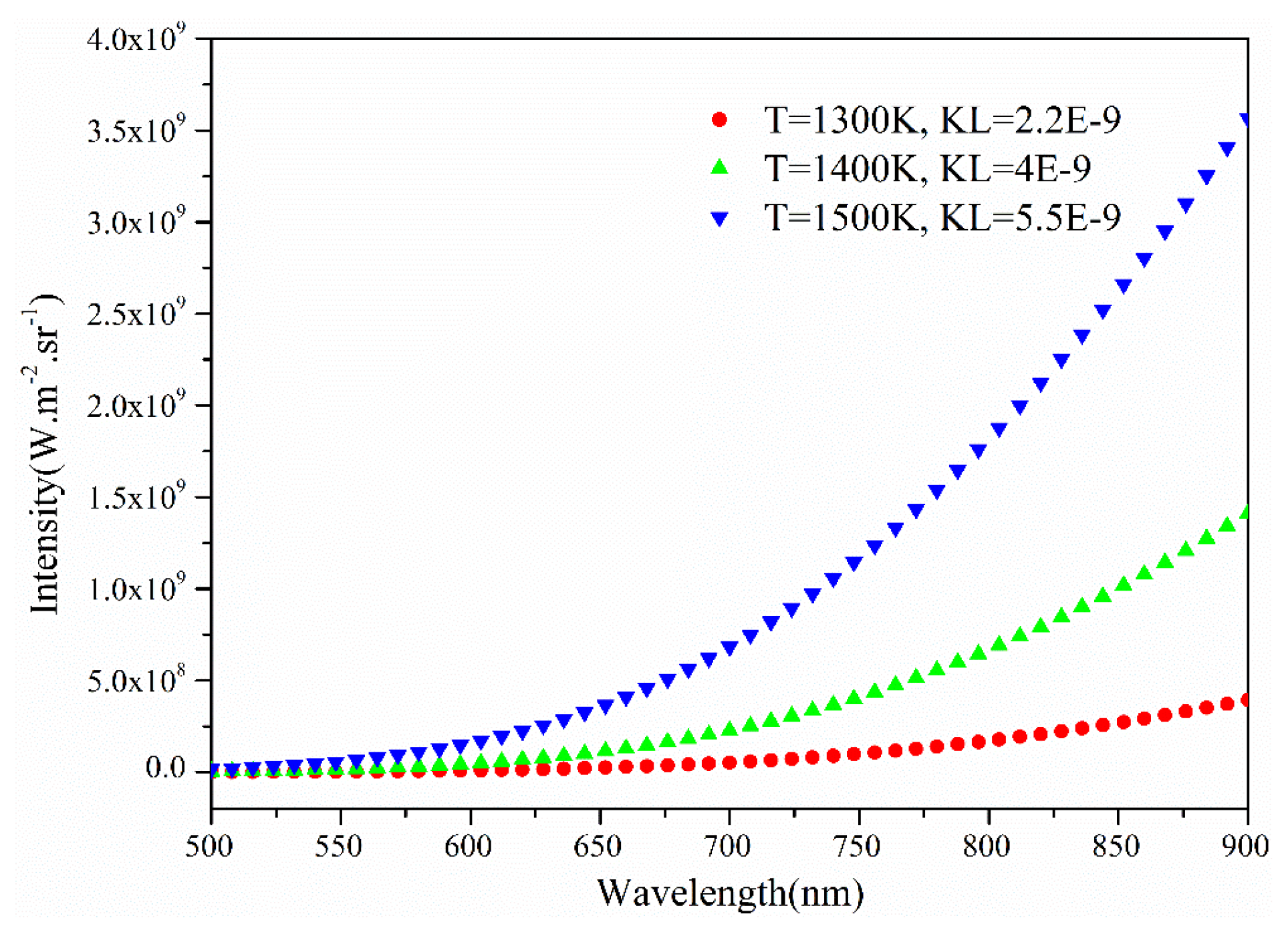
The Hottel and Broughton emissivity model was used to test the accuracy of the method. Three groups of hypothesis values of
KL and
T were used to obtain a simulated continuous spectral baseline by integrating Plank’s Law, as shown in
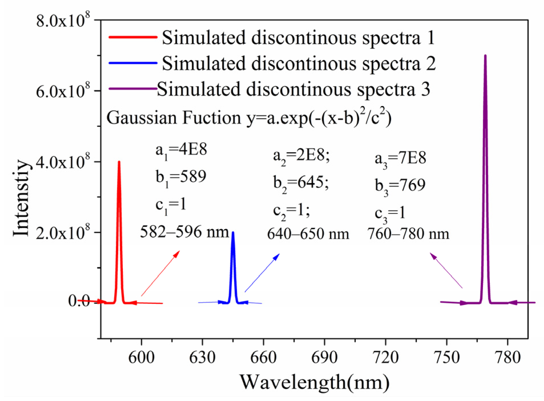
Figure 1. Three simulated discontinuous emission bands were assumed based on a Gaussian function, as shown in
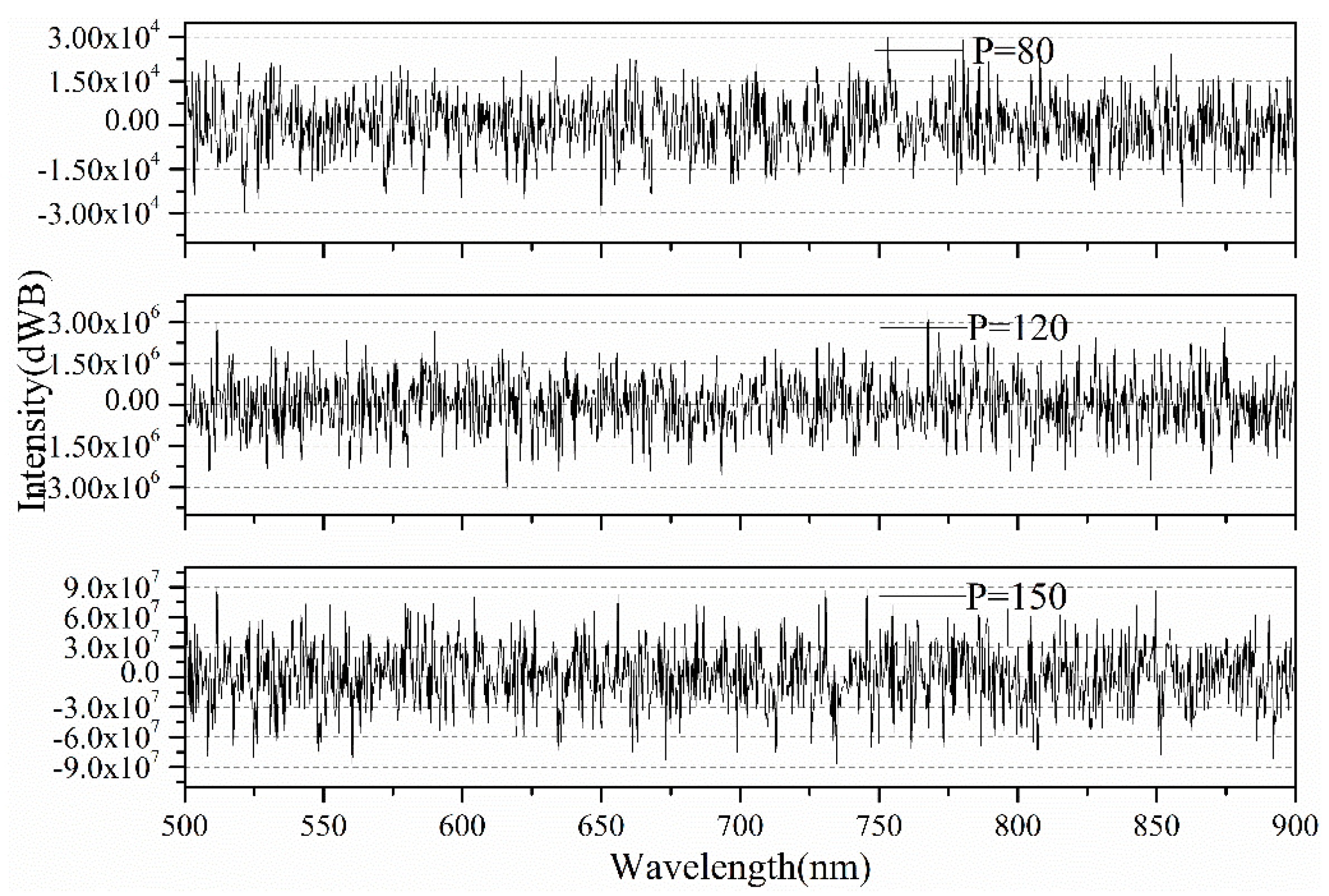
Figure 2. Three types of white noise determined by the WGN (white Gaussian noise) function in Matlab (R2012a, The MathWorks, Inc., Natick, MA, USA) were used as simulated spectrometer noise, as shown in
Figure 3. The power of the output noise at 80, 120, and 150 dBW was denoted by the capital letter P. Nine synthetic spectra were obtained by the combination of different simulated baselines, and the simulated discontinuous bands and the types of simulated noise were considered as the measured flame spectra, as shown in
Figure 4. The wavelength interval of the simulated baseline, the discontinuous bands, and the noise between two adjacent wavelengths was set to 0.5 nm to facilitate a spectral synthesis.
There are nine synthetic spectra with different baselines and different types of white noise. The proposed method for separating the continuous baseline from the measured spectra was used to obtain the estimated continuous spectrum. A nonlinear least squares method was applied to calculate the inverse temperature
KL1 and
T1. The comparison between the predicted values of
KL,
T, and the inverse calculated
KL1 and
T1 values are shown in
Table 1. The relative error of the predicted and inverse calculated values is also presented. The synthetic spectra with low white noise generally have a high accuracy. As the white noise increased, the accuracy of this method decreased. Furthermore, the stronger the intensity of the hypothesis baseline, the higher the precision for the inverse calculated
KL1 and
T1 is. This implies that the signal-to-noise ratio (SNR) will affect the accuracy of the method. For this example, the effect of the SNR is greater for
KL than for
T. However, for most synthetic spectra, the influence on the calculated
KL and
T values is acceptable. We conclude that the proposed method for separating the continuous and discontinuous spectra under a high SNR is appropriate.
3. Spectroscopic System and Calibration Introduction
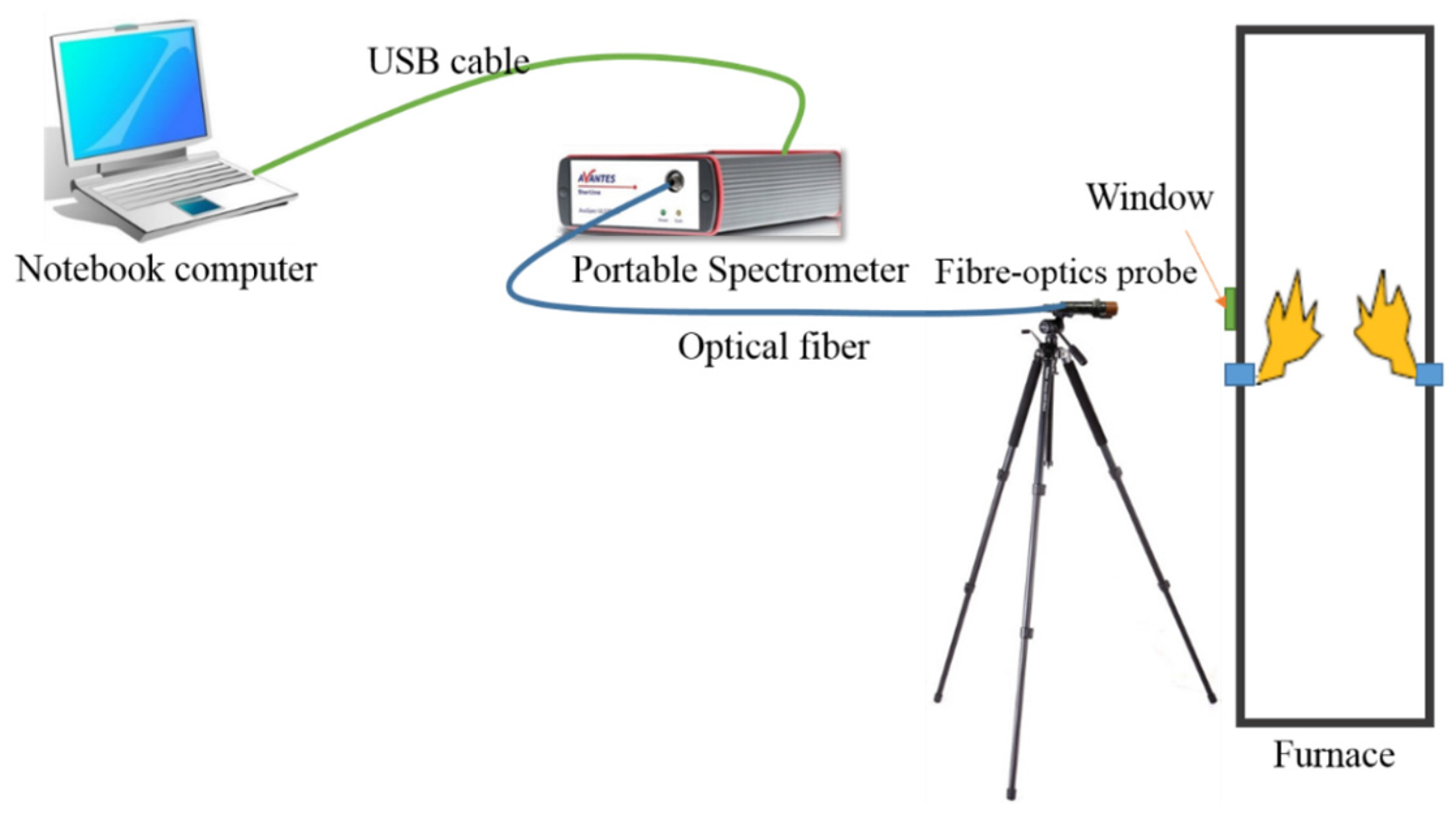
The spectrometer system includes a laptop, universal serial bus (USB) data cable, portable spectrometer, optical fiber, fiber optic probe, and triangle bracket used for fixing the fiber optic probe (
Figure 5). An AvaSpec-ULS2048-USB2 with a 2048 pixel CCD (Charge-coupled Device) detector array is used to process the incoming light data. A choice of 15 different gratings with different dispersions and blaze angles enables applications in the 200–1100 nm range. The fiber-optic spectrometer’s integration time ranges from 1.1 to 600 ms, and the resolution of the spectrometer is 0.1 nm. During the measurement, the flame radiation is projected to an optical fiber after lens convergence and the signal is transmitted to the CCD fiber-optic spectrometer by optical fiber; subsequently, the obtained flame radiation spectrum signal is input into a computer for processing.
A spectrometer system is used to obtain the monochromatic radiation intensity within a certain wavelength range. However, the signal output from the spectrometer is a voltage signal converted by photoelectric conversion [
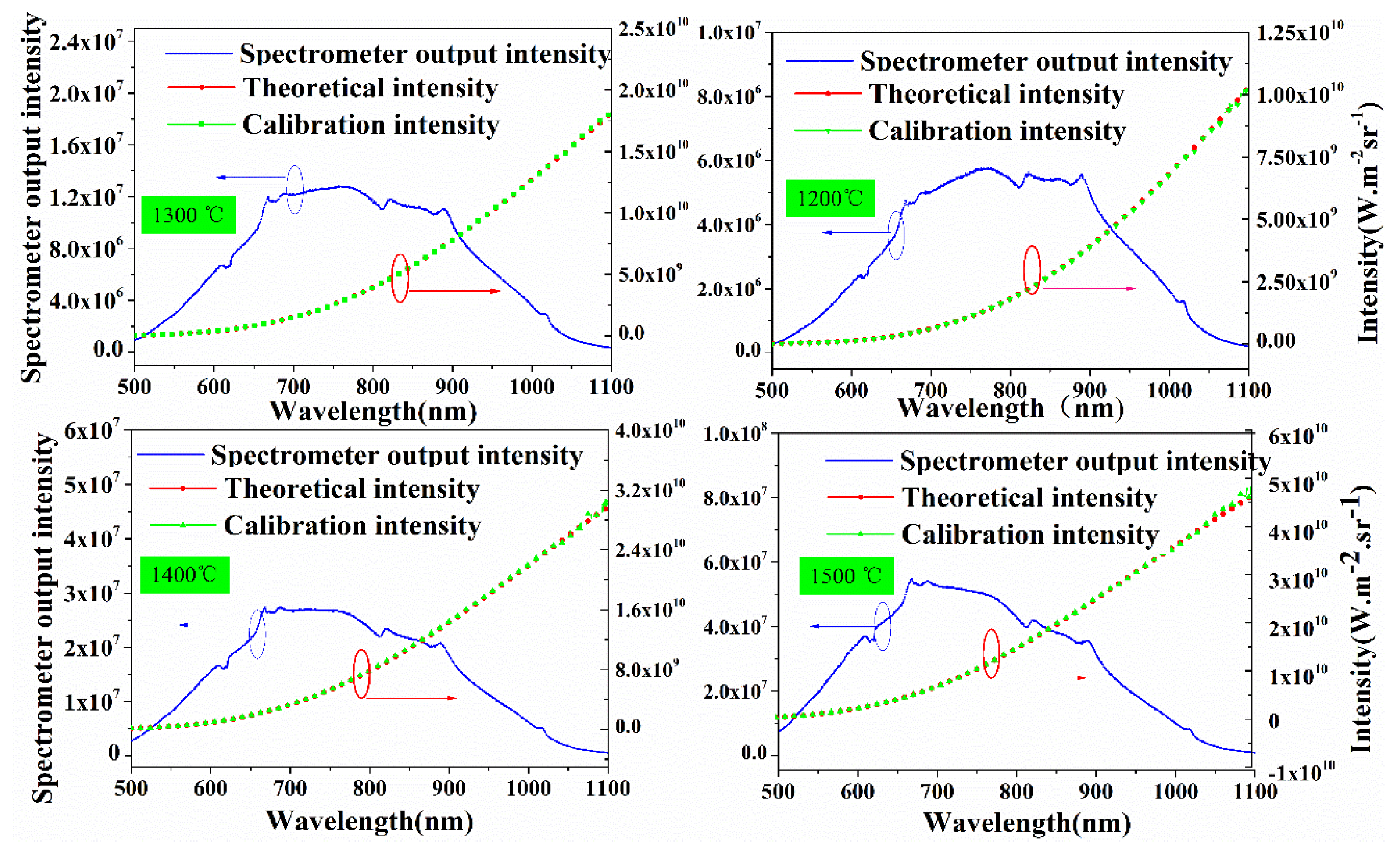
13]. To obtain the monochromatic radiation intensity, a calibration is required for spectrometer output values. A blackbody furnace with a temperature range from 300 °C to 1700 °C, model Mikron M330, is used for the calibration. The calibration factor as a function of
λ yields the performance calibration curve with a wavelength ranging from 500 to 1100 nm at five temperatures of 1100°C, 1200°C, 1300°C, 1400°C, and 1500 °C.
In order to verify the accuracy of the calibration, the results before and after correction for 1100 °C and 1400 °C are shown in
Figure 6, which shows that the measured spectral curves and the corrected curves are consistent with the theoretical results. The theoretical blackbody radiation intensity after calibration is essentially coincident with the blackbody radiation intensity at temperatures of 1200 °C, 1300 °C, 1400 °C, and 1500 °C, indicating that the calibration is accurate.
4. Experimental Setup and Procedure
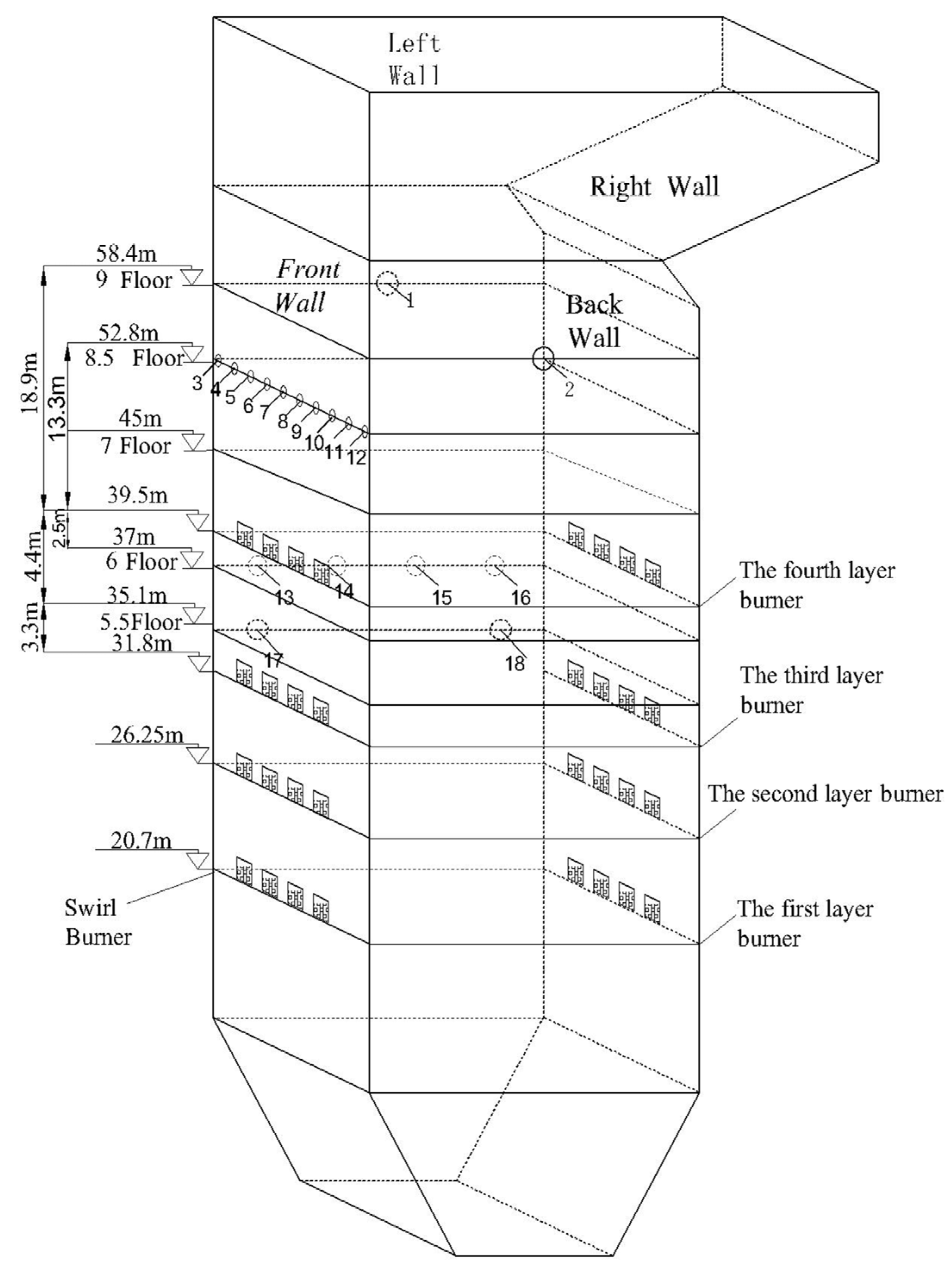
The measurements were conducted in a 1000 MW supercritical coal-fired boiler at the Huadian International Zouxian Power Plant. The boiler furnace has four layers of swirl burners and uses the opposed wall firing method, as shown schematically in
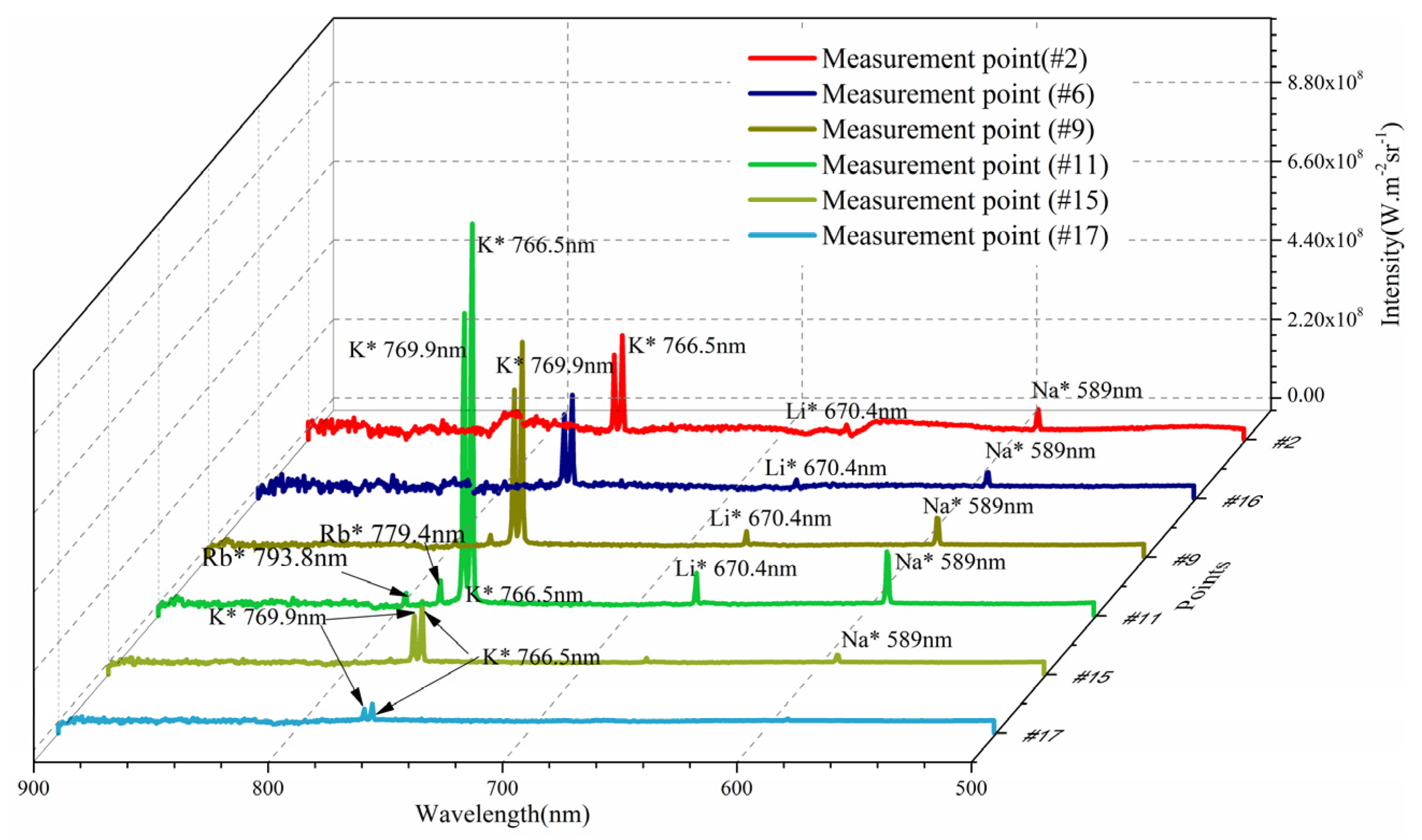
Figure 7. In each layer, eight burners are equally distributed on the front and back furnace walls. The measurement points positioned in the 5.5 layer of the left wall were numbered #1 and #2; the measurement points in the 6 layer of the left wall were numbered #3, #4, #5, and #6; and the measurement points located in the 8.5 layer of the front wall were numbered #7, #8, #9, #10, #11, #12, #13, #14, #15, and #16. Finally, the measurement points in the center hole of the left and right wall in the 9 layer were numbered #17 and #18. The layers of the burners numbered from bottom to top were called the first, second, third, and fourth layer. The distance between the 9 layer and the fourth layer of the burners is 18.9 m, and there is a distance of 13.3 m from the 8.5 layer to the fourth layer of the burners. The 6 layer is 2.5 m from the fourth layer of the burners. All of the described layers are at the top of the fourth layer of the burners; however, the 5.5 layer is located between the third layer of the burners and the fourth layer of the burners. The measurement points of the 5.5 layer are close to the third distribution layer of the burners and the distance is 3.3 m.
During the measurements, the boiler load of the unit remained unchanged and the 1000 MW unit operated at 992 MW. The spectrometer measurements were performed at different locations in the unit. The raw output data from the spectrometer system was calibrated and used for the spectral analysis and calculation of the flame’s temperature and emissivity. During spectrum acquisition, the optical fiber probe was placed perpendicular to the wall of the observation points. The measurement points in the unit were named from bottom to top to facilitate the analysis and discussion. To reduce the measurement error caused by the disturbance of the pulverized coal flame when measuring each point, multiple groups of spectral data were collected at each measurement point and the average value of the flame radiation intensity for the points under the same boiler load was calculated.
6. Conclusions
A fiber-optic spectrometer was used for the diagnosis of a 1000 MW coal-fired power plant boiler furnace. The calibration of the spectrometer was conducted in a blackbody furnace to obtain the calibration coefficient, and the accuracy of the calibration coefficient was confirmed.
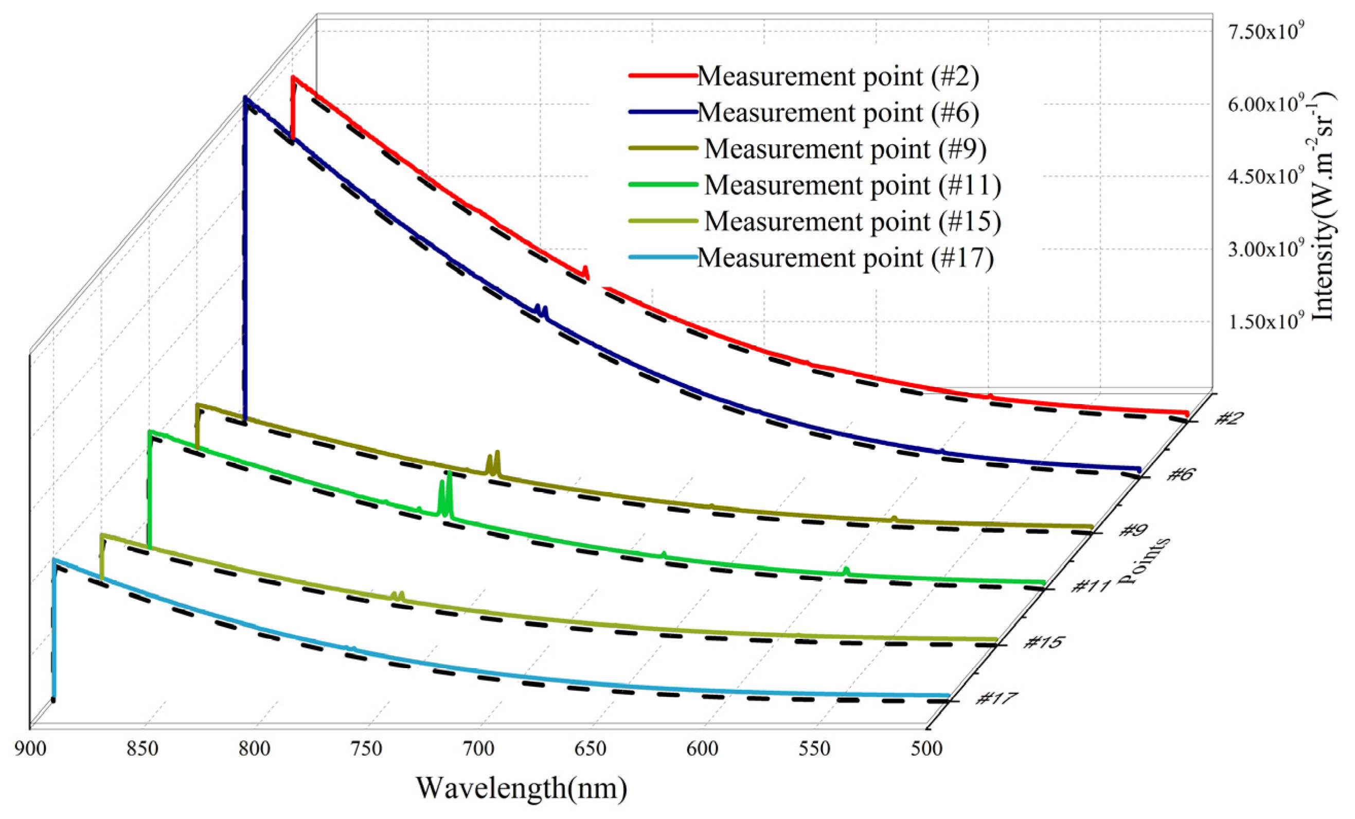
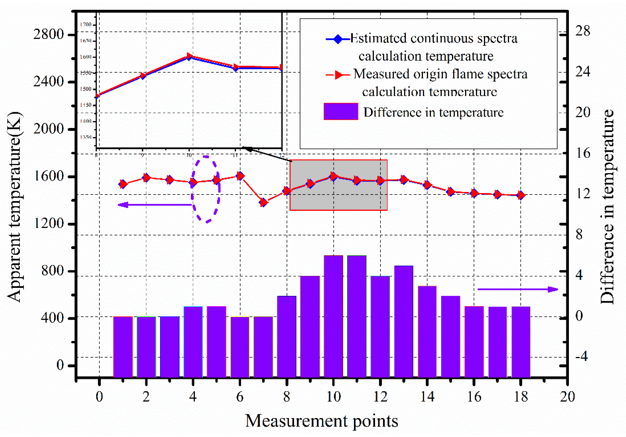
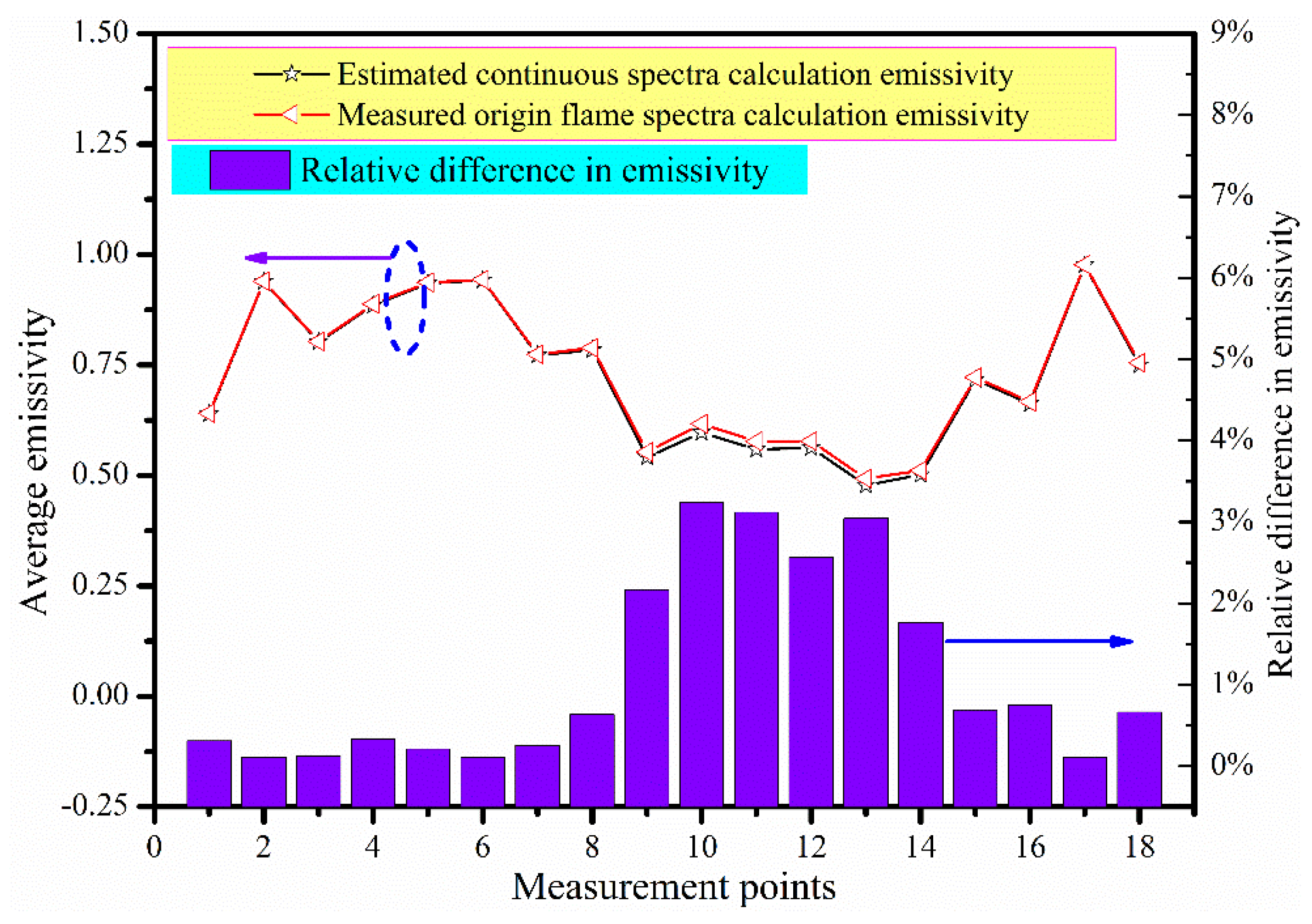
A simple method was proposed to separate the baseline from the continuous and discontinuous spectra. The accuracy of the estimated continuous baseline derived from the measured flame spectra was evaluated by the goodness-of-fit coefficient and satisfactory agreements were achieved for the selected profiles. The influence of the discontinuous emission spectra on the calculations of temperature and emissivity for several observation points was evaluated for a coal-fired flame. There was little difference in the calculated temperature and emissivity based on the estimated continuous spectra and the emitted flame spectrum, and the maximum difference for the temperature for all measurement points was only 6 K. The impact on emissivity was very small and similar to the influence on the calculated temperature, and the relative difference in emissivity at all points was less than 5%.
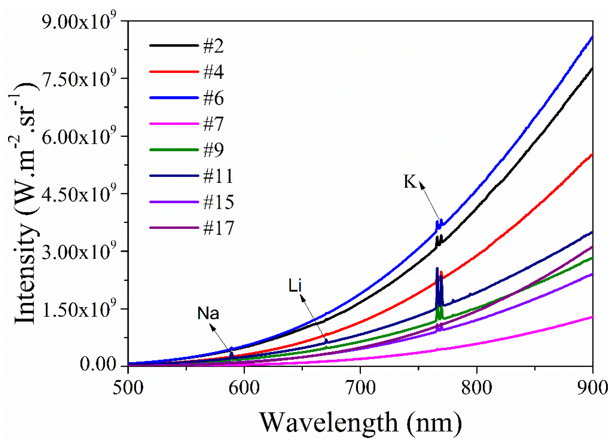
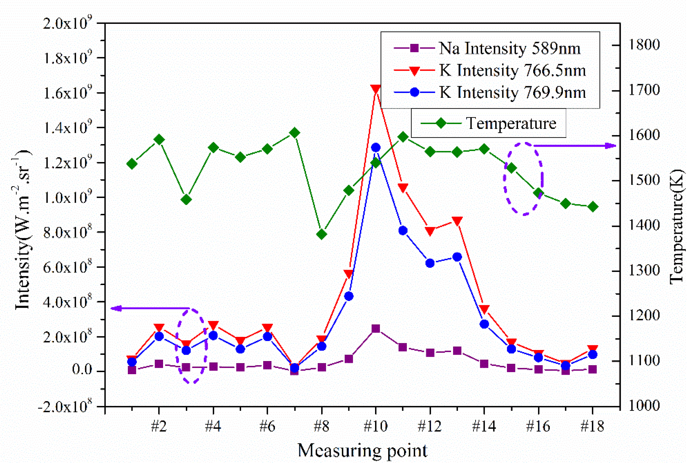
A comparison between the actual intensity of the alkali metal and the calculated temperature indicated that the change in the radiation intensity of the alkali metal followed the trend of the calculated temperature. However, this was not consistent with the relationship between the radiation intensity of the alkali metal and the calculated temperature. This implies that the radiation intensity of the alkali metal is related to the measurement location of the flame’s temperature and the alkali metal concentrations.


