A Personalized Rolling Optimal Charging Schedule for Plug-In Hybrid Electric Vehicle Based on Statistical Energy Demand Analysis and Heuristic Algorithm

Abstract

To alleviate the emission of greenhouse gas and the dependence on fossil fuel, Plug-in Hybrid Electrical Vehicles (PHEVs) have gained an increasing popularity in current decades. Due to the fluctuating electricity prices in the power market, a charging schedule is very influential to driving cost. Although the next-day electricity prices can be obtained in a day-ahead power market, a driving plan is not easily made in advance. Although PHEV owners can input a next-day plan into a charging system, e.g., aggregators, day-ahead, it is a very trivial task to do everyday. Moreover, the driving plan may not be very accurate. To address this problem, in this paper, we analyze energy demands according to a PHEV owner’s historical driving records and build a personalized statistic driving model. Based on the model and the electricity spot prices, a rolling optimization strategy is proposed to help make a charging decision in the current time slot. On one hand, by employing a heuristic algorithm, the schedule is made according to the situations in the following time slots. On the other hand, however, after the current time slot, the schedule will be remade according to the next tens of time slots. Hence, the schedule is made by a dynamic rolling optimization, but it only decides the charging decision in the current time slot. In this way, the fluctuation of electricity prices and driving routine are both involved in the scheduling. Moreover, it is not necessary for PHEV owners to input a day-ahead driving plan. By the optimization simulation, the results demonstrate that the proposed method is feasible to help owners save charging costs and also meet requirements for driving.

1. Introduction

In recent years, plug-in hybrid electric vehicles (PHEVs), as eco-friendly and cost-effective transportation vehicles [1], have drawn world-wide attention [2,3]. By shifting from fuel power to battery power, electric driven vehicles are not only helpful to reduce the emission of green-house gas but also have a considerable energy independence. Therefore, many countries’ governments, auto manufacturing enterprises, and energy enterprises have paid lots of attention to the development of PHEVs. For one thing, compared to the fossil-fuel vehicle, electric power is much friendlier to the environment and the price is much cheaper, since renewable energies generated by wind or solar have nowadays been common in the smart grid [4]. For the other, PHEVs are generally affordable for long distance driving while the pure electric vehicle is poor in endurance.

Because of the fluctuation of electricity spot prices in the power market, it is viable to create a charging schedule for PHEV to save costs and also meet PHEV owners’ driving requirements. However, it is a big challenge to integrate EVs (electrical vehicles) into the current smart grid due to many different kinds of factors such as grid load burden, investments of infrastructures, revenue of customers, etc. In [5], Green et al. investigated the influences of EVs charging to the distribution network and concluded that the key factors include driving patterns, charging characteristics, charging time, and vehicle penetrations. Belgium, as an example, was investigated in detail to explore the impacts from EVs to such networks [6]. For charging characteristics, a fast but unregulated charging of EVs will lead to a heavy grid load burden, moreover, even cause a breakdown of power system [7]. In addition, as indicated by the technical reports from the Oak Ridge National Laboratory and the National Renewable Energy Laboratory [8,9], an uncontrolled charging strategy will also cause an additional demand of generation capacities. Hence, to enhance the benefits of using EVs, it is necessary to optimize charging control strategies for EVs. In recent years, to address the issues, various kinds of charging control strategies have been proposed and applied substantially [10,11].

From the perspective of the power provider, the research generally focuses on the optimization of grid load or power losses. To minimize power losses and maximize the grid load factor, a coordinated charging schedule strategy was proposed by Clement et al. [12]. In [13], Sundstrom and Binding considered the issue that involves multiple EVs. From the view of PHEV owners, Jin et al. considered both aggregators’ revenue and drivers’ demand on energy to conduct the research to propose offline and online charging scheduling strategies for multiple EVs [4]. By investigating the elasticity of EV loads, Gan et al. proposed a decentralized charging schedule strategy to fill the valleys in electric load profiles [14]. In [15], the authors proposed a lottery-based charging strategy to decide whether to charge an EV or not, in order to guarantee fairness.

As an intermediary part between vehicle owners and grid operators, aggregators have played a significant role in executing smart charging for EVs [16] and also have actively taken place in the electricity market [17]. The optimization problems on the aggregators’ side have been widely investigated in recent years. In [18], a dynamic programming was employed in frequency formulation to propose an optimal charging strategy for each vehicle to maximize aggregators’ revenue. A fleet of EVs are modelled by aggregate battery approaches and a charging scheduling optimization by dynamic programming-based method were proposed by Skugor and Deur [19]. In [7], the authors investigated a maximization problem to pursue aggregators’ profit by controlling the optimal charging rates. In [4], the benefits of both the electricity provider and vehicle owners are considered by linear programming. Aggregators are also well used for the researches on power market. A contract size about frequency of regulation was optimized in [20] based on the historically obtained probability distribution of procured power capacity. In [21], by employing fuzzy optimization, an optimal bidding of ancillary services coordinated across different markets are researched. An improved heuristic algorithm named particle swarm optimization was proposed in [22] to exploit the potential consumers value added by coordinated distributed energy resource scheduling.

Besides the aggregators’ revenue, in EV charging problems, there also exist many other perspectives on optimization objectives. For the battery energy storage system (BESS) charging scheduling problem, Maly and Kwan employed a dynamic programming to minimize the electricity bill while reducing battery stress and prolonging battery life [23]. To reduce payment and operational costs, intelligent scheduling for charging/discharging, as a crucial step to implement EVs to smart grid, has also been widely studied [24,25]. In [26], charging cost and grid load are taken into account to be minimized by a hierarchical schedule for vehicle fleets. In [27], the authors proposed two linear programming models for different kinds of optimization objectives including maximization of vehicle owners’ revenue and maximization of the number of EVs fulfilling their requirements. In addition to linear programming, various kinds of other programming approaches are also employed to optimize the schedule for electric vehicles. In [28], the authors considered a total cost of a large scale EVs by quadratic programming. A heuristic algorithm was used to address a large scale PHEVs charging scheduling problem aiming at the objective of maximizing the average state-of-charge [29]. In [10], the authors employed estimation of distribution algorithm (EDA) to well address the 3000 PHEVs charging scheduling problem and obtained satisfactory optimization results. In [30], a suite of computational intelligence-based algorithms are adopted to address the problems. Other than the optimization methods, there also exist various kinds of optimization objectives, such as the minimization of charging cost, minimization of grid load variance, maximization of aggregators’ profit, maximization of average state-of-charge of vehicles, and many others. A summary on the optimization objectives can be found in [31]. Nevertheless, for the above studies, there still exist the problems below.

• The research that is on the side of power providers does not consider the owners’ personalized demand on electricity energy as well as the payment for charging in a dynamic environment of electricity spot prices.
• Much research on charging schedules requires the day-ahead energy demand, which means the owners should input the next-day driving plan everyday. However, it is trivial for owners. Besides, it is difficult to ensure the accuracy of plan.

By considering both charging payments and daily driving routines simultaneously, in this paper, a rolling dynamic optimization for PHEV charging is proposed. A heuristic algorithm termed Biogeography-based Optimization (BBO) is adopted to address the charging scheduling problem. In this paper, we divide one day into $N=24$ time slots. Namely, each time slot sustains one hour. For a more accurate schedule, it is also feasible to divide one day into more time slots. For the charging problem, the schedule system will consider both forward electricity prices (the prices in the following 24 time slots) and the historical driving routine. Based on the information, the system will decide whether to charge the vehicle or not in the current time slot. The decision for the current time slot will be made according to the optimized schedule. However, the schedule will be remade in the next time slot since refreshed spot prices (a refreshed 24 prices in the following time slots) will be provided. Hence it is a dynamic rolling optimization problem.

Heuristics are very popular in dealing with optimization problems in current decades. Xue employed an artificial bee colony algorithm to handle global optimization and obtained competitive performances for global optimization [32]. Zhang et al. employed heuristic algorithms to wireless sensor networks and was copied well with the energy conservation problem in the process data gathering [33]. A heuristic strategy was employed in dealing with the privacy problem in social network data sharing, which showed the heuristics’ superiority [34]. For multi-objective optimization, heuristic algorithms also play a crucial role. Liu employed NSGA-II to a heterogeneous cloud system and obtain a comprehensive view for decision makers [35]. In addition, for the idea of heuristics, it is usually employed in many different kinds of searching and exploration strategies. In [36], Xia used the heuristic idea to propose a “Greedy Depth-first Search”, which was well implemented to multi-keyword ranked search scheme and well optimized the time complexity of algorithms. All the achievements of heuristics demonstrate it is a powerful tool to address optimization problems. For scheduling problems, heuristic algorithms are also very active. Compared with the programming methods, heuristic algorithms have several advantages summarized below.

• Heuristic algorithms are independent of problems. After encoding operation (e.g., binary encoding, matrix encoding, etc.), the run of the algorithm is independent to the problem. The final results can be obtained by decoding operation. Hence, the design of algorithms and the proposal of problems are separable, which provides a favourable compatibility for an algorithm’s application.
• For heuristic algorithms, they do not need much mathematical information. Compared with several traditional mathematical methods, such as programming methods, it is impossible to solve optimization problems without derivative information of objective function.
• It is more adaptive to employ heuristic algorithm to solve different kinds of optimization problems including multi-modular optimization problems, dynamic optimization problems, linear programming problems, dynamic programming problems, integer programming problems, and so forth. Hence, even if some conditions in the problems change, heuristic algorithms are still competent to address them.

In this paper, we investigate the charging schedule from the owners’ perspectives and conduct rolling optimization for charging schedule by heuristic algorithms. First, to avoid the cumbersome task of daily input to a driving plan, we built a model of driving routine according to historical driving records, which brings two advantages: (1) it is needless to input the next-day plan, which can provide a smart charging service. The drivers only input specific driving plans if needed; (2) Since the driving routine is modeled according to owners’ habits, the charging schedule is personalized. Second, we will conduct a dynamic optimization per time slot, which means that the schedule will be made according to the changes of real driving routine autonomously.

The remainder of this paper is organized as follows. In Section 2, the current day-ahead power market is introduced in brief. In Section 3, we build the model for owners’ driving habits and make the charging scheme based on the driving routine model. Specifically, in Section 3.1, the owners’ habit will be illustrated. A statistical model for energy demand in different time slots is built, which is a combinatorial optimization problem in a dynamic environment. In Section 3.2, to address the optimization problem, an evolutionary algorithm is employed to design a charging scheme to minimize the owners’ payments for energy demand. The simulation experiments are conducted in Section 4. The simulation results are also analyzed to provide suggestions for owners. We conclude this paper in Section 5 and present our future work.

2. Background and Preliminaries

2.1. A Brief of the Power Trading Market

As a kind of wholesale electricity market in Scandinavia, the day-ahead market operated by Nordpool is the main arena for trading power. In this market, electricity production balance the responsible party (seller) and the consumption responsible party (buyer) to reach an energy agreement for the delivery of power on the following day. With this agreement, the spot price is set and the trade is agreed. This daily trading is driven by the seller and buyers’ planning. For example, the buyer needs to assess how much energy he will need to meet the demand of the following day, and how much it is willing to pay for this volume, hour by hour. The seller needs to decide how much he can deliver and at what price, hour by hour.

After having these plans, they will submit their bids to Nordpool before 12:00 AM everyday. Then, the Nordpool will publish the hourly spot price one hour later, i.e., all the players in the market will know the spot price for the following day. However, due to the increasing penetration of uncertain renewable energy as well as the displacement of conventional generation, it will further increase the needs of real time balancing resources. Thus, the uncertainty issue should be considered when making the schedule and the fluctuation of spot prices also provides the space for optimization to save the charging cost.

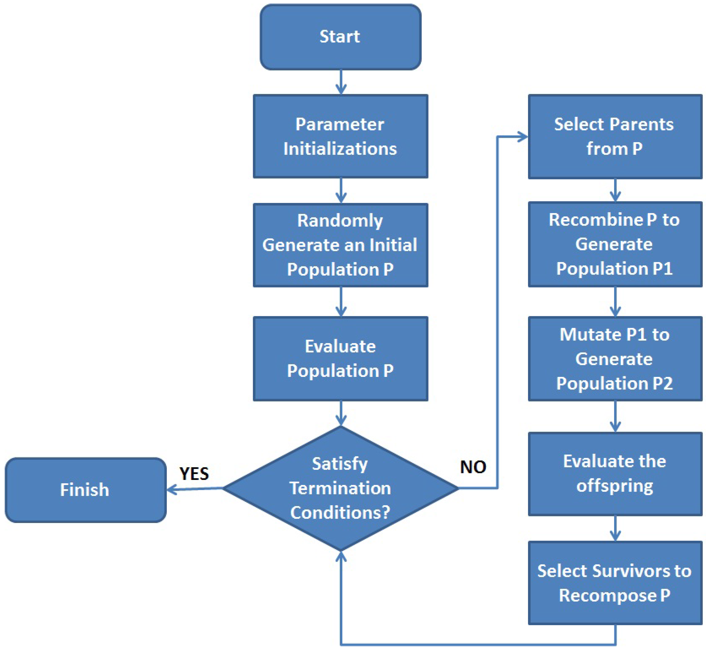
2.2. Preliminary of Heuristic Algorithm

The charging scheduling problem is a combinatorial optimization problem. To address these kinds of problems, the heuristic algorithm plays a very active role. In general, heuristic algorithms are inspired from natural phenomena, and have now drawn much attention from worldwide researchers. For the algorithms, they are usually independent of the background of optimization problems but only focus on the optimization objectives and searching space. Therefore, they are well and widely applied to many areas including engineering, finance, medicine, transportation, and so forth [37,38]. The famous heuristic algorithms include the Genetic Algorithm (GAs) [39], Differential Evolution (DE) [40], Ant Colony Optimization (ACO) [41], Biogeography based Optimization (BBO) [42], and many others. As mentioned in Section 1, heuristic algorithms are already well used in charging problems with different kinds of optimization objectives and constraints, which demonstrates the algorithms are competent in addressing optimization problems in the EV power market. In general, there are three components in the design of algorithms, which are recombination operator, crossover operator, and selection operator. A general design flowchart of the heuristic algorithm is given in Figure 1.

Most differences among heuristic algorithms exist generally in the design of the recombination operator. In GA, the crossover operator recombines different candidate solutions by mimicking the natural genetic mechanism in biology [39]. BBO designs the migration operator to enforce the communication among different candidate solutions by simulating species migration among different islands [43]. DE produces new offsprings by the differences of their parents [40]. ACO explores the searching space by the cooperation among ants’ cooperation [41]. The various kinds of recombination operators have their own properties in addressing different optimization problems. In this paper, BBO will be employed to optimize the optimization in PHEV’s charging scheme. For BBO, it has a more flexible way to recombine candidate solutions since for each recombination all candidates are involved, while for GA only one pair of candidates are in one recombination [43,44]. In addition, BBO is easily implemented since it has few parameters in programming, compared with several other heuristic algorithms such as ant colony optimization (ACO) [41] that contains around five parameters.

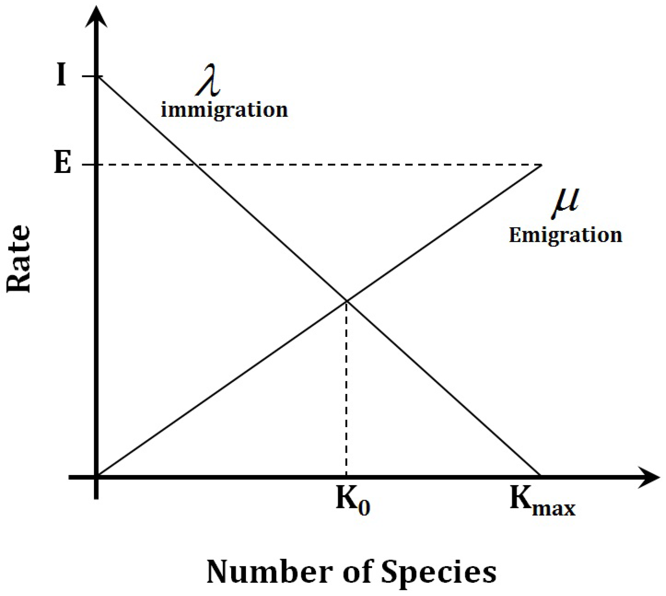
2.3. Brief of Biogeography-Based Optimization

Biogeography-based Optimization (BBO) mimics the species migration among different islands. In the algorithm, candidate solutions are analogous to islands. For fertile islands, there are a huge number of species living there, while for barren islands, only a few of species live there. Considering there are lots of species living in a fertile island, it is difficult to immigrate to the islands and species’ trend is to emigrate. While for barren islands, the immigration rate is high and emigration rate low. Inspired from this idea, the good solutions have a large emigration rate and a low immigration rate, while the poor solutions have a low emigration rate and a high immigration rate. Moreover, a large emigration rate means the solution will much affect other solutions. On the other hand, a large immigration rate means the solutions will be much affected by other solutions. A figure to illustrate the migration rates is given in Figure 2.

Figure 2 illustrates a linear model of species distribution in a single habitat [43], where I is the maximum possible immigration rate and E represents the maximum possible emigration rate. The immigration rate $\lambda$ and the emigration rate $\mu$ are functions of the number of species in the habitat. For one island, the immigration rate increases and the emigration rate decreases as the number of species increases. As a very important operator in EAs, the mutation operator helps algorithms break away local optima and maintain population diversity. In BBO [43], the mutation rate is calculated by (1).

$$m_K=m_{max}\left(\frac{{\mu }_{max}-{\mu }_K}{{\mu }_{max}}\right)$$

(1)

where K is the index of candidate solution, $m_{max}$ is defined by users in advance, ${\mu }_K$ are the immigration probability calculated according to migration model, and ${\mu }_{max}$ is the maximal immigration rate of $\mu$. A linear migration model is shown in Figure 2. Compared with many other conventional evolutionary algorithms, the mutation rate in BBO fluctuates over the course of the optimization process, which is affected by the recombination operator, say the migration operation. A detailed analysis on BBO’s mutation rate can be found in [45]. The psudo-codes of BBO are given in Algorithm 1.

Algorithm 1: Pseudo-codes of Biogeography-based Optimization.

3. Design for Charging Scheme

Due to the fluctuated electricity prices, a satisfactory charging scheme is useful for PHEV owners to save charging costs and also meet the requirements of a driving plan. For the driving routine, in general, the owners should input the next day driving plan into charging system, e.g., aggregators. However, it is a very trivial task for drivers. Besides, in general, the plan may not be very accurate. Hence, in this section, a driving schedule will be conducted through modeling on historical driving records. After that, the driving model and the electricity prices in the next 24 time slots (24 h) will be employed as input of evolutionary algorithms for scheduling. We chose Biogeography-based Optimization to solve the corresponding optimization problem because of its straightforward implementation and ability to generate optimal schedules within manageable computation times.

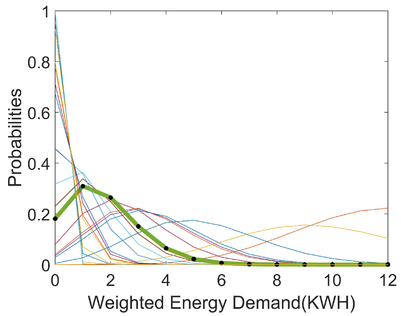
3.1. Modeling of Energy Demand

In this section, according to PHEV owner’s historical driving routine, a statistical model is built. In the modeling, several assumptions are made below.

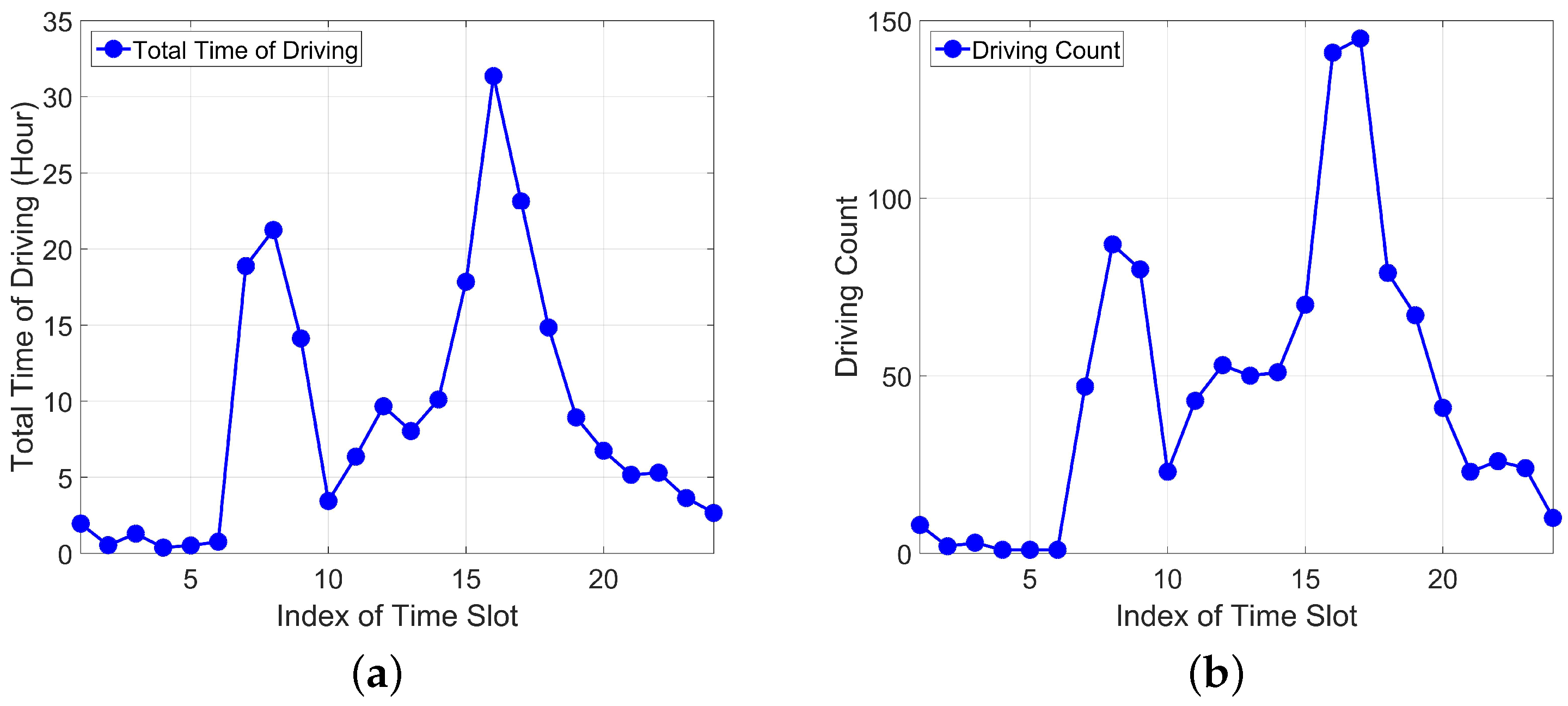
• We divide one day into N time slots. For each time slot, there are only two charging status, the charging status and non-charging status. For the non-charging status, it includes two cases. The first case is the idle case that means there is neither charging nor discharging. The second case is discharging when driving. We do not schedule for the time slot where the vehicle is driven. Even if the driving operation does not occupy a whole time slot, we consider the whole time slot as used for driving and do not conduct scheduling on the rest of that time slot.
• In any full time slot, we consider the energy consuming is E, which means that we employ an average energy demand per time slot regardless of the road condition or accelerating/decelerating status. For the time slot that is not fully occupied by charging time, we calculate the energy cost proportionally to the driving time.

By analyzing driving data in $\Theta =246$ days, total $\Omega =1074$ driving records are obtained. Due to the limitation of pages, we only present segmental part including 20 records in

Table 1. 20 driving records from total 1074 records. Each record presents the complete time cost for a driving record. Start Time is the time to start driving, while Finish Time records the end time.

Trip Number	Start Time		Finish Time
1	2001/12/7	16:07:38	2001/12/7	16:18:55
2	2001/12/7	16:25:52	2001/12/7	16:46:22
3	2001/12/7	17:05:52	2001/12/7	17:18:47
4	2001/12/7	17:48:06	2001/12/7	17:49:57
5	2001/12/7	18:00:45	2001/12/7	18:09:51
6	2001/12/8	10:31:02	2001/12/8	10:36:52
7	2001/12/8	10:51:53	2001/12/8	10:57:29
8	2001/12/8	11:04:00	2001/12/8	11:05:09
9	2001/12/8	11:26:36	2001/12/8	11:31:29
10	2001/12/8	11:55:51	2001/12/8	11:55:53
11	2001/12/8	12:09:09	2001/12/8	12:17:00
12	2001/12/9	10:32:17	2001/12/9	10:36:14
13	2001/12/9	13:35:47	2001/12/9	13:40:48
14	2001/12/10	06:32:14	2001/12/10	06:58:57
15	2001/12/10	15:27:37	2001/12/10	15:41:10
16	2001/12/10	15:48:42	2001/12/10	16:08:54
17	2001/12/11	06:33:45	2001/12/11	06:59:00
18	2001/12/11	15:31:53	2001/12/11	15:57:37
19	2001/12/11	16:07:49	2001/12/11	16:12:11
20	2001/12/11	16:28:16	2001/12/11	16:30:37

. “Start Time” is the time that owner begins to use the vehicle, while the “Finish Time” records the end time that finish the driving.

As mentioned above, in this paper, we divide one day into 24 time slots, namely $N=24$ and therefore for each time slot, the time is $T_{Interval}$ of one hour. The driving time during the j-th time slot is calculated according to (2).

$$T_j=\left\{\begin{array}{c}\sum _{i=1}^{\Omega }\left(F_t\left(i\right)-S_t\left(i\right)\right),if{S}_t\left(i\right),F_t\left(i\right)\in slot\left(j\right)\hfill \\ \sum _{i=1}^{\Omega }\left(F_t\left(i\right)-S_{slot\left(j\right)}\right),if{S}_t\left(i\right)\notin slot\left(j\right)\&F_t\left(i\right)\in slot\left(j\right)\hfill \\ \sum _{i=1}^{\Omega }\left(F_{slot\left(j\right)}-S_t\left(i\right)\right),if{S}_t\left(i\right)\in slot\left(j\right)\&F_t\left(i\right)\notin slot\left(j\right)\hfill \\ \sum _{i=1}^{\Omega }\left(F_{slot\left(j\right)}-S_{slot\left(j\right)}\right),if{S}_t\left(i\right),F_t\left(i\right)\notin slot\left(j\right)\&F_t\left(i\right)>F_{slot\left(j\right)}\&S_t\left(i\right)<S_{slot\left(j\right)}\hfill \end{array}\right.$$

(2)

where $T_j$ is the total time cost during the jth time slot, $\Omega =1074$ is the amount of driving records, $F_t\left(i\right)$ and $S_t\left(i\right)$ ($i\in [1,\Omega ]$) are finish time and start time for a driving, $slot\left(j\right)$ ($j\in [1,N]$) is the jth time slot, and $F_{slot\left(j\right)}$ and $S_{slot\left(j\right)}$ are the finish time and start time of the jth time slot. In (2), there are four cases. For the first case, the finish time and start time of the i-th driving are both in $slot\left(j\right)$. For the second case, the start time of the i-th driving is not in the $slot\left(j\right)$, but the finish time of the i-th driving is in the $slot\left(j\right)$. For the third case, the start time of the i-th driving is in the $slot\left(j\right)$, but the finish time of the i-th driving is not in the $slot\left(j\right)$. For the fourth case, the whole driving time covers $slot\left(j\right)$, which leads to the result that both finish time and start time of the i-th driving are not in the time slot $slot\left(j\right)$. By statistical analysis, the total time for driving in each time slot is given in Figure 3a. Besides, we also employ, in a similar way as (2), to calculate the driving accounts in each time slot and present the statistical results in Figure 3b. According to the figures, it is obvious that in a day, there are two peaks occurring during 7:00–9:00 a.m. and 16:00–18:00 p.m., which corresponding with daily rush hours.

As mentioned in the first item of assumptions, the energy consuming is proportional to the driving time. It consumes energy E for a full time slot. According to the statistical results of driving time, we can evaluate energy cost for each time slot. However, there exits some rare driving behaviors that should be properly dealt with. In the statistical analysis of Figure 3a and Figure 3b, there exit some sporadic driving actions. For example, according to Figure 3a, during the time slot 3 (from 3:00 a.m. to 4:00 a.m.), the total driving time is about one hour. However, during the time slot, there only exists few driving records in total 1074 records. Hence, we consider the driving action as sporadic driving, which is not a habitual routine. To reduce the influence of happenstance to driving routine modeling, we employ $\phi$ shown in (3) as a weight to evaluate the corresponding energy demand $e_d$ for each time slot.

$${\phi }_{e_d}\left(i\right)=\frac{coun{t}_{e_d}\left(i\right)}{\Theta }$$

(3)

where $coun{t}_{e_d}$ is the energy demand $e_d$ that occurs in the i-th time slot and $i\in \{1,2,\dots ,24\}$, $\Theta =264$ is the total days of records . For the energy demand $e_d$, it is proportional to the time consuming, which is given in (4).

$$e_d=\frac{T_{e_d}}{T_{interval}}\times E$$

(4)

where $T_{e_d}$ is the time cost to consume energy $e_d$, $T_{interval}$ is the time duration of a full time slot, and in this paper the value of $T_{interval}$ is one hour. The weighted energy demand $e_w$ at the i-th time slot is given in (5).

$$e_w\left(i\right)=\sum _{j=1}^{coun{t}_i}{\phi }_{e_d}\left(j\right)\times e_d\left(j\right).$$

(5)

where $coun{t}_i$ is the total number of driving records in the i-th time slot, $i\in [1,2,\dots ,24]$. According to (5), the weighted energy consumption shows the energy cost in habitual daily driving routine. An example to explain the weight is given as follows. In the statistical analysis of 246 days, for the time slot of 3:00 a.m. to 4:00 a.m., there exists a driving behavior using about 40 minutes only once and therefore it costs energy of $\frac{2}{3}E$. Since such driving at that time only exists once during 246 days, the weight value $\phi$ is $\frac{1}{246}$ and therefore the weighted energy demand is $e_w\left(\frac{2}{3}E\right)=\frac{1}{246}\frac{2}{3}E$. Hence, $e_w\left(\frac{2}{3}E\right)$ is a very small value and is also competent to reflect the true routine in PHEV owners’ daily life. By accumulating all weighted energy demands in each time slot, we define the weighted energy demand in the i-th time slot in (6).

$$D\left(i\right)=\sum _{i=1}^{\Omega }{e}_w\left(i\right)$$

(6)

where $e_w\left(i\right)$ is obtained by (5), $i\in [1,2,\dots ,24]$. By defining $E=12$ kWh, for the energy demand in each time slot, we draw the figures shown in Figure 4.

According to the figure, on one hand, it is obvious that there is nearly no energy cost during the nights and also reflect the two period of peak consuming at 8:00 a.m. and 16:00–17:00 p.m., which reflect the personalized true habitual driving routine. On the other hand, the y-axis is the energy consumption. It is easy to know the energy demand in each time slot. For the energy consumption in each time slot, it meets the Poisson probability distribution, which is given in (7).

$$P(i,j)=\left(\frac{e_w{\left(i\right)}^j}{j!}\right)\ast exp(-e_w\left(i\right))$$

(7)

where $i\in [1,2,\dots ,24]$ is the index of time slot and j is the number of $e_w$. The figures to show the probability distribution of energy demands in 24 time slots are given in Figure 5. Each curve presents the probabilities in each corresponding time slots.

In Figure 5, we employ the bold green curve as an example to explain the meaning. For the green curve, it presents the probabilities at the time slot 19:00–20:00. According to the green curve (at the time slot 19:00–20:00), the probability of energy demand “1 kWh” is about 0.35. The probability of energy demand “2 kWh” is 0.28. The probability of energy demand “0 kWh” is about 0.2. The probability of energy demand “4 kWh” is about 0.6. The green curve only presents the probabilities of different energy demand for time slot 19:00–20:00. Other curves present the probabilities of energy demands in different time slots. In the charging scheduling, we select the energy demand with the maximum probability as a predictive energy demand.

3.2. Design of Optimization for Charging Schedule

To pursue a minimal payment, a charging schedule is designed in this subsection. The optimization objective is given in (8).

$$\begin{array}{cc}\hfill \mathit{Minimize}P& =\sum _{i=1}^{24}C\left(i\right)\times S\left(i\right)\hfill \\ \hfill St.B\left(i\right)& \ge D\left(i\right)\hfill \end{array}$$

(8)

where P is the total payment in the future 24 time slots, $C\left(i\right)$ as a binary integer is used to depict the charging status at the i-th time slot, $S\left(i\right)$ is the spot price at the i-th time slot, and $B\left(i\right)$ is the dump energy in battery at i-th time slot. Since the maximum state of battery is 12 kWh, the maximal value of $B\left(i\right)$ is 12, $D\left(i\right)$ is the demand at the i-th time slot, and $B\left(i\right)=B(i-1)+C(i-1)$. Thanks to the day-ahead electric market, we assume that the $S\left(i\right)$s in the next 24 time slots are known in advance. According to (8), it is a constrained optimization problem. To solve the constraints, we employ the penalty function method. The penalty function is designed according to the price of gasoline, which means that once the electric power is not enough for driving, the user must pay the price of gasoline for vehicle endurance, which is feasible for PHEVs. Hence the optimization objective is modified in (9).

$$\mathit{Minimize}P=\sum _{i=1}^{24}C\left(i\right)\times S\left(i\right)+max\{D\left(i\right)-B\left(i\right),0\}\times S_g$$

(9)

where $S_g$ is the price of gasoline. Since in this paper, we assume the output power remains unchanged, the cost of $S_g$ in different time slot is also fixed. Here we assume $S_g$ is 9 Euro per hour. According to (9), this problem can be considered as a combinatorial optimization problem. In addition, the optimization environment is dynamically changing per hour.

As explained above, we employ a heuristic algorithm named Biogeography-based Optimization (BBO) to address the dynamic rolling optimization problem. As a heuristic algorithm, it is powerful to address combinatorial optimization problems. For optimization, we conduct a rolling dynamic schedule for charging, which means that the schedule is made every hour from the current time slot to the next 24 h. The charging decision in current time slot is made according to the optimization schedule. The inputs include the electric prices and the weighted energy demands in the following 24 h. However, at the next time slot, the schedule is remade according to the new inputs in the following 24 h, which is a rolling schedule. The steps of optimization is given as follows.

• Record the electricity spot prices $P=\left[P\right(1),P(2),\dots ,P(24\left)\right]$ per time slot in the next 24 time slots (hours).
• Record the weighted energy demand $E_w=[e_w\left(1\right),e_w\left(2\right),\dots ,e_w\left(24\right)]$ per time slot in the next 24 time slots (hours).
• Input P and $E_w$ (total 48 decision variables) to BBO for optimization according to Algorithm 1.
• Output the charging decision for each time slot in the next 24 h.

The pseudo codes of the algorithm are presented in Algorithm 2.

Algorithm 2: Pseudo-codes of BBO for Personalized Charging Schedule.

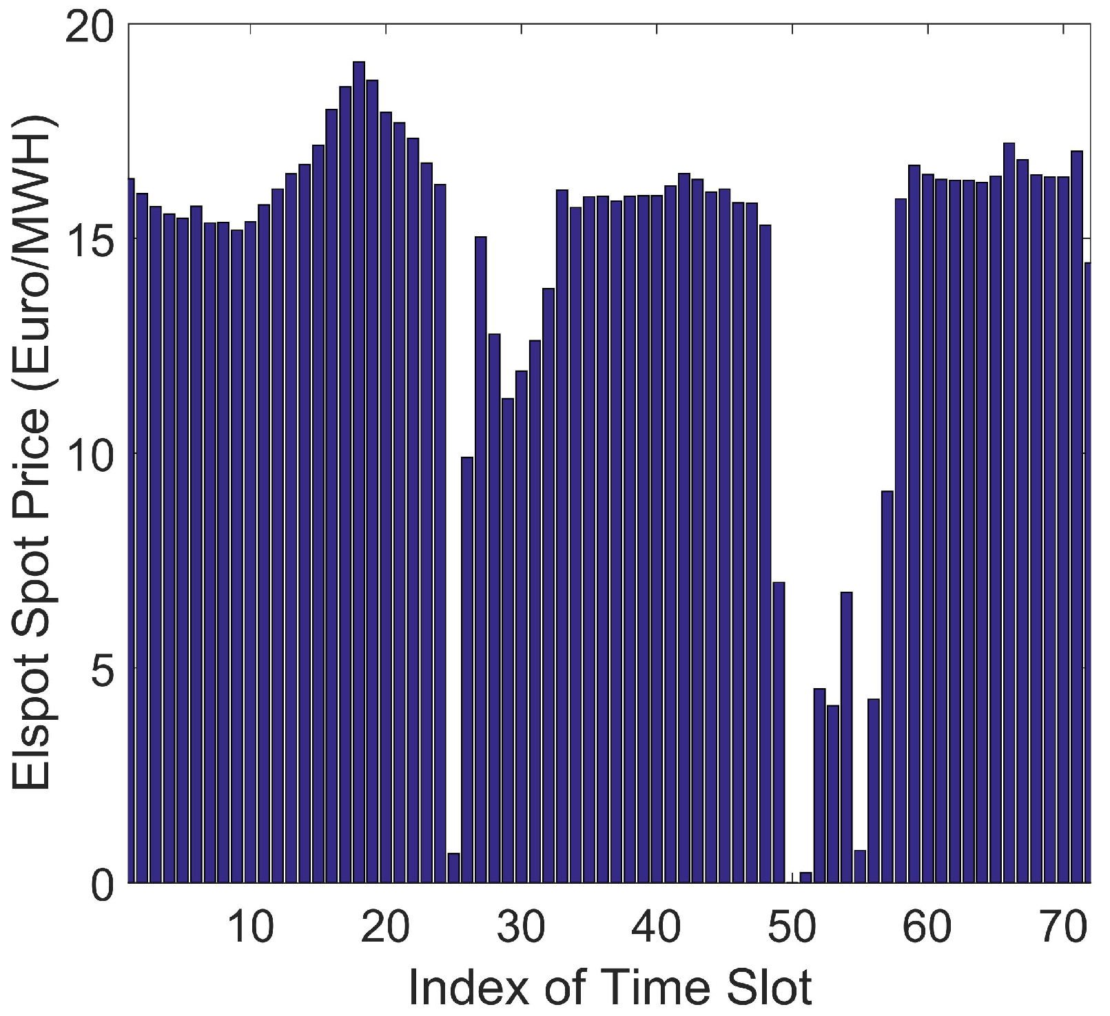
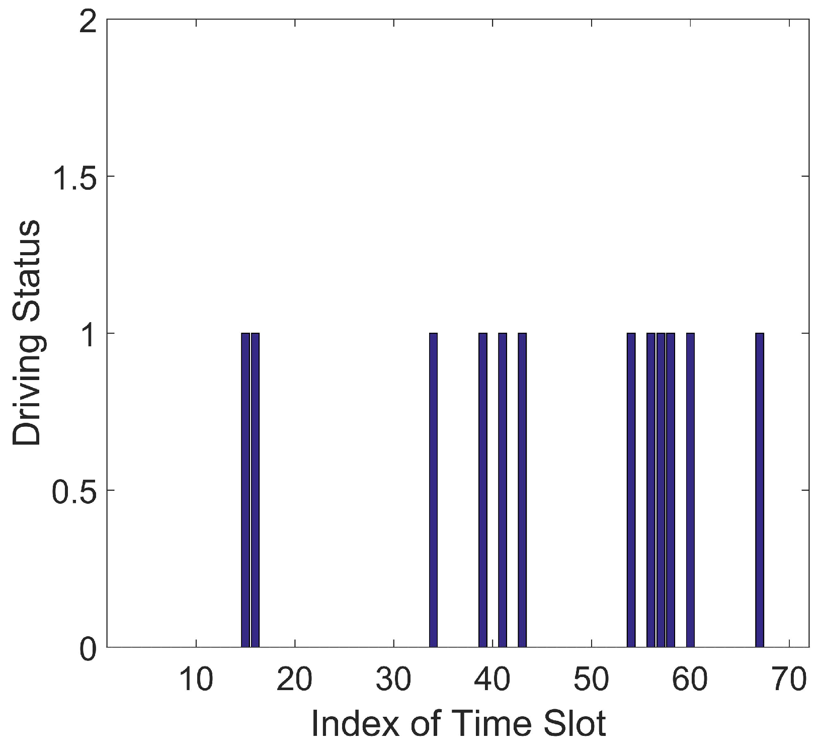
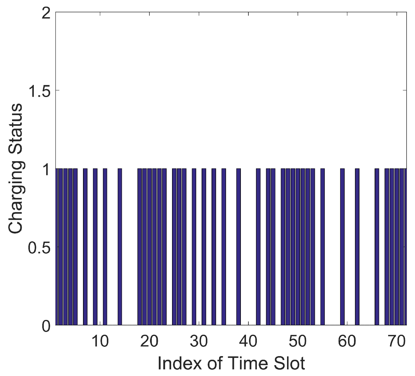
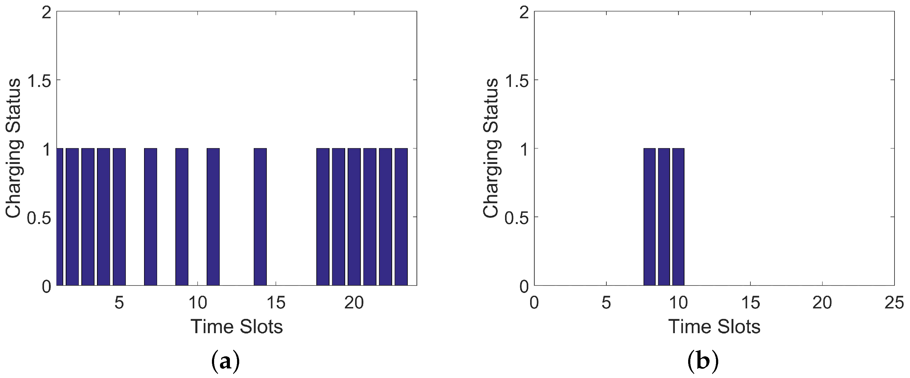
4. Simulation and Discussion

In this section, according to the modeling in Section 3.1, we consider the statistical model as a predicted by energy demand and input the electricity prices in the next 24 h to the optimization algorithm. The charging schedule is given as follows. The capacity of the battery is 12 kWh which means that if the battery is fully charged, the charging schedule cannot set the charge status as a ’1’. The rated charging power is set as 2 kWh. In the initial stage, there is no power in battery. The start time is from 0:00 at the first day, while the end time is at 24:00 at the third day. The price of gasoline is set as €1.4 per liter (Price in Denmark as reference), and for each time slot (one hour) the driving cost of gasoline is about €9. We run the simulations in a computer with a CPU of Intel(R) Core(TM) i5-4300U @ 1.9 GHz and the compiler is Matlab 2016a in Windows 7 SP 1. For the heuristic algorithm BBO, we employ a population size of 50 and set the generation limitation as 100, which means the limitation of fitness evaluations is $100\times 50=5000$. For the migration operator, a linear model is employed and the mutation rate is 0. We run the algorithm for 25 times and the average time cost for calculation is round 4.27 (±0.21) s. Considering that in this paper time slot is one hour, which means the charging schedule should be conducted hourly, it is definitely timely to do the calculation in seconds. The electricity prices of the 72 time slots are given in Figure 6, which were downloaded from an official website http://osp.energinet.dk/_layouts/Markedsdata/framework/integrations/markedsdatatemplate.aspx. The predictive energy demand is calculated by (7), according to the historical driving data and the real energy demand is given in Figure 7.

In the simulation, in addition to BBO, we also employ other two well-known heuristic algorithms, which are the genetic algorithm (GA) and ant colony optimization (ACO) respectively, as peer algorithms for a performance comparison. The population size in the two algorithms is also set as 50 and the maximum fitness evaluations is also set as 5000 to guarantee a fair comparison. For GA, a roulette wheel selection mechanism is employed. We select a single-point selection in the crossover operator and the crossover probability is 1, and a mutation rate is set as 0.01. For ACO, we used the following parameters; initial pheromone value is as $1\times {10}^{-5}$; pheromone update constant is 20; exploration constant is set as 1; global pheromone decay rate is 0.9; local pheromone decay rate is 0.5; pheromone sensitivity is 1; and visibility sensitivity is 5. For each algorithm, we run the algorithm 25 times to obtain an average performance. The convergence performances of the three algorithms are presented in Figure 8a. For each run, the averaged time cost is 4.27 (±0.21) s, 4.12 (±0.19) s, and 5.33 (±0.17) s for BBO, GA, and ACO, respectively. It is noticed that in Figure 8a, it is only one optimization process and as a rolling optimization process. In total, there are 72 figures since the algorithms will be executed for each time slot. Due to the limitation of pages, we only present one figure for the 1st time slot as an example. The charging scheduling for the 1st time slot (from 0:00 to 1:00 a.m.) is given in Figure 8b, where “0” is the non-charging status and “1” is the charging status. According to Figure 8b, the decision in the current time slot (the 1st time slot) is “charging”. Hence, we make the decision “charging” as the current operation. A comparison of the algorithm’s performance charging cost (best performance, mean performance and worst performance) and averaged running time, are summarized in

Table 2. Performance comparisons for algorithms GA, ACO, and BBO. “Best”, “Mean”, and “Worst” are the minimal cost, averaged cost, and maximal cost, respectively, in 25 runs for each algorithm.

Algorithm Names	Charging Cost (€)			Averaged Run Time (Seconds)
	Best	Mean	Worst
GA	1.87	1.89	1.96	4.27
ACO	1.83	1.85	1.91	5.33
BBO	1.71	1.72	1.74	4.12

. “Best” is the minimal cost in 25 runs for each algorithm, “Mean” is the averaged cost in 25 runs, and “Worst” is the maximal cost calculated by algorithms in 25 runs.

As shown in Figure 8a, BBO has a very competitive convergence pressure and also outperforms other two algorithms, which demonstrates that BBO is competitive to address the charging scheduling problems for electrical vehicles. According to Table 2, BBO outperforms other two well-known heuristic algorithms ACO and GA. To be specific, BBO does not only have the best performance for “Best”, “Mean”, and “Worst” results in 25 independent runs, but also has the smallest computation time. Hence, the choice of BBO is very competitive to deal with the optimization problem. For all the charging status for 72 time slots, we present the Figure 9, and the total price is about €1.71. All driving demands are met and there is no driving using gasoline fuel. In this paper, we present the charging status in 72 h but not a long-term schedule. The reasons are given below. First, as mentioned, it is due to the pages limitation. Second, in this paper, the rolling optimization is a short-term schedule. On one hand, the price of electricity power can be known only before one day. It is not possible to do a long-term schedule (more than 24 h). In this paper, the presented 72 h performance is based on the historical data but not a real-time and practical scheduling. On the other hand, the historical data is always updated. A benefit of the rolling optimization is that this schedule is conducted according to a driver’s historical routine. However, general routine may change for different months or seasons. Hence, even if a longer time schedule is conducted, it may not be much helpful for practical use. In addition, with the fluctuation of energy demand in different months or seasons, the errors in rolling optimization always exists. Therefore, in our view, it is not fair to compare the rolling optimization performance to the scheduling with an accurate pre-input plan, which is a trivial task for drivers.

An error analysis on energy demand is presented in Figure 10. In Figure 10a, the schedule obtained by the proposed algorithm BBO is shown, while Figure 10b is a charging schedule according to a real driving routine in 24 h by mixed-integer linear programming.

From the two figures, the charging schedules are obviously different and reasons are generally from three aspects. First, it is definitely different between a fixed-plan charging schedule and a rolling charging schedule. For a fixed-plan charging schedule, it will not consider the afterward driving demand, while the rolling charging schedule will consider more on the next dozens of time slots. The different kinds of charging perspectives cause different ways to charge vehicles. In rolling optimization, although a schedule of 24 h is made, only the decision in the current time slot is adopted. A second factor is the estimating error. The Poisson probability provides a statistical analysis for users’ driving behavior. However, in the real world, the owners will not always obey his or her usual habits. For fixed plan charging, the schedule can be made more accurately. Nevertheless, the accurate schedule may not be robust, which means once the plan changes, the fixed plan cannot provide a promising endurance for driving. Third, the difference is from the modeling of scheduling. In this paper, the scale of time slot is one hour, which means an operation of “driving" will take a whole time slot, even the real driving time is only a few minutes. For the remaining time in such time slots, we do not conduct any charging operation. Hence, the idle time will also cause a systematical error.

5. Conclusions

In this paper, we propose a novel idea for PHEV charging for personalized customers. By analyzing historical driving records, we built a PHEV charging model, which correspond to the PHEV owners’ historical driving routine. By employing the model, a heuristic algorithm named BBO is used to optimize the charging schedule. The schedule is made according to the energy demand and the spot prices in near future. According to the simulation results, the proposed approach is feasible and effective.

In our future work, the time slot will be divided into minutes to pursue a more accurate optimization schedule. However, with the minutes schedule, it may encounter the problem that there will exist a considerable error between a PHEV owner’s driving action and the predicted driving model. To apply the proposed approach to vehicle fleets that include tens and hundreds of vehicles, more customized requirements for daily driving routines of different vehicles will be considered as well as for a large scale charging schedule and it is mandatory to consider the grid load. In addition, in this paper, the proposed strategy is for the drivers’ party by conducting the optimization according to owners’ driving routine. Our future work will consider the limitations of the distribution network, which involves more factors including network congestion, bus voltage drop, transformer overloading, and so forth.

References

1. Akbari, H.; Fernando, X. Modeling and optimization of PHEV charging queues. In Proceedings of the 2015 IEEE 28th Canadian Conference on Electrical and Computer Engineering (CCECE), Halifax, NS, Canada, 3–6 May 2015; pp. 81–86. [Google Scholar]
2. Guo, F.; Inoa, E.; Choi, W.; Wang, J. Study on Global Optimization and Control Strategy Development for a PHEV Charging Facility. IEEE Trans. Veh. Technol. 2012, 61, 2431–2441. [Google Scholar] [CrossRef]
3. Dong, Q.; Niyato, D.; Wang, P.; Han, Z. The PHEV Charging Scheduling and Power Supply Optimization for Charging Stations. IEEE Trans. Veh. Technol. 2016, 65, 566–580. [Google Scholar] [CrossRef]
4. Jin, C.; Tang, J.; Ghosh, P. Optimizing Electric Vehicle Charging: A Customer’s Perspective. IEEE Trans. Veh. Technol. 2013, 62, 2919–2927. [Google Scholar] [CrossRef]
5. Green, R.C.; Wang, L.; Alam, M. The impact of plug-in hybrid electric vehicles on distribution networks: A review and outlook. Renew. Sustain. Energy Rev. 2011, 15, 544–553. [Google Scholar] [CrossRef]
6. Clement-Nyns, K.; Haesen, E.; Driesen, J. The Impact of Charging Plug-In Hybrid Electric Vehicles on a Residential Distribution Grid. IEEE Trans. Power Syst. 2010, 25, 371–380. [Google Scholar] [CrossRef] [Green Version]
7. Sortomme, E.; El-Sharkawi, M.A. Optimal Charging Strategies for Unidirectional Vehicle-to-Grid. IEEE Trans. Smart Grid 2011, 2, 131–138. [Google Scholar] [CrossRef]
8. Denholm, P.; Short, W. An Evaluation of Utility System Impacts and Benefits of Optimally Dispatched Plug-In Hybrid Electric Vehicles; Technical Report for National Renewable Energy Laboratory: Golden, CO, USA, 2006. [Google Scholar]
9. Hadley, S.W. Impact of Plug-In Hybrid Vehicles on the Electric Grid; Technical report for Oak Ridge National Laboratory: Oak Ridge, TN, USA, 2006. [Google Scholar]
10. Su, W.; Rahimi-Eichi, H.; Zeng, W.; Chow, M.Y. A Survey on the Electrification of Transportation in a Smart Grid Environment. IEEE Trans. Ind. Inform. 2012, 8, 1–10. [Google Scholar] [CrossRef]
11. Mukherjee, J.C.; Gupta, A. A Review of Charge Scheduling of Electric Vehicles in Smart Grid. IEEE Syst. J. 2015, 9, 1541–1553. [Google Scholar] [CrossRef]
12. Clement, K.; Haesen, E.; Driesen, J. Coordinated charging of multiple plug-in hybrid electric vehicles in residential distribution grids. In Proceedings of the 2009 IEEE/PES Power Systems Conference and Exposition, Seattle, WA, USA, 15–18 March 2009; pp. 1–7. [Google Scholar]
13. Sundstrom, O.; Binding, C. Flexible Charging Optimization for Electric Vehicles Considering Distribution Grid Constraints. IEEE Trans. Smart Grid 2012, 3, 26–37. [Google Scholar] [CrossRef]
14. Gan, L.; Topcu, U.; Low, S.H. Optimal decentralized protocol for electric vehicle charging. IEEE Trans. Power Syst. 2013, 28, 940–951. [Google Scholar] [CrossRef]
15. Vasirani, M.; Ossowski, S. A Computational Monetary Market for Plug-In Electric Vehicle Charging. In Proceedings of the Auctions, Market Mechanisms, and Their Applications: Second International ICST Conference (AMMA 2011), New York, NY, USA, 22–23 August 2011; Coles, P., Das, S., Lahaie, S., Szymanski, B., Eds.; Springer: Berlin/Heidelberg, 2012; pp. 88–99. [Google Scholar]
16. Bessa, R.J.; Matos, M.A. Global against divided optimization for the participation of an EV aggregator in the day-ahead electricity market. Part I: Theory. Electr. Power Syst. Res. 2013, 95, 309–318. [Google Scholar] [CrossRef]
17. Pecas Lopes, J.A.; Soares, F.J.; Rocha Almeida, P.M. Integration of Electric Vehicles in the Electric Power System. Proc. IEEE 2011, 99, 168–183. [Google Scholar] [CrossRef]
18. Han, S.; Han, S.; Sezaki, K. Development of an Optimal Vehicle-to-Grid Aggregator for Frequency Regulation. IEEE Trans. Smart Grid 2010, 1, 65–72. [Google Scholar]
19. Skugor, B.; Deur, J. Dynamic programming-based optimisation of charging an electric vehicle fleet system represented by an aggregate battery model. Energy 2015, 92, 456–465. [Google Scholar] [CrossRef]
20. Jang, S.; Han, S.; Han, S.H.; Sezaki, K. Optimal decision on contract size for V2G aggregator regarding frequency regulation. In Proceedings of the 2010 12th International Conference on Optimization of Electrical and Electronic Equipment, Brasov, Romania, 20–22 May 2010; pp. 54–62. [Google Scholar]
21. Ansari, M.; Al-Awami, A.T.; Sortomme, E.; Abido, M.A. Coordinated bidding of ancillary services for vehicle-to-grid using fuzzy optimization. IEEE Trans. Smart Grid 2015, 6, 261–270. [Google Scholar] [CrossRef]
22. Pedrasa, M.A.A.; Spooner, T.D.; MacGill, I.F. Coordinated Scheduling of Residential Distributed Energy Resources to Optimize Smart Home Energy Services. IEEE Trans. Smart Grid 2010, 1, 134–143. [Google Scholar] [CrossRef]
23. Maly, D.K.; Kwan, K.S. Optimal battery energy storage system (BESS) charge scheduling with dynamic programming. IEE Proc. Sci. Meas. Technol. 1995, 142, 453–458. [Google Scholar] [CrossRef]
24. Li, F.; Qiao, W.; Sun, H.; Wan, H.; Wang, J.; Xia, Y.; Xu, Z.; Zhang, P. Smart Transmission Grid: Vision and Framework. IEEE Trans. Smart Grid 2010, 1, 168–177. [Google Scholar] [CrossRef]
25. Shireen, W.; Patel, S. Plug-in Hybrid Electric Vehicles in the smart grid environment. In Proceedings of the 2010 IEEE PES Transmission and Distribution Conference and Exposition: Smart Solutions for a Changing World, New Orleans, LA, USA, 19–22 April 2010. [Google Scholar]
26. Xu, Z.; Hu, Z.; Song, Y.; Zhao, W.; Zhang, Y. Coordination of PEVs charging across multiple aggregators. Appl. Energy 2014, 136, 582–589. [Google Scholar] [CrossRef]
27. Kuran, M.S.; Viana, A.C.; Iannone, L.; Kofman, D.; Mermoud, G.; Vasseur, J.P. A Smart Parking Lot Management System for Scheduling the Recharging of Electric Vehicles. IEEE Trans. Smart Grid 2015, 6, 2942–2953. [Google Scholar] [CrossRef]
28. He, Y.; Venkatesh, B.; Guan, L. Optimal Scheduling for Charging and Discharging of Electric Vehicles. IEEE Trans. Smart Grid 2012, 3, 1095–1105. [Google Scholar] [CrossRef]
29. Su, W.; Chow, M.Y. Performance evaluation of a PHEV parking station using Particle Swarm Optimization. In Proceedings of the 2011 IEEE Power and Energy Society General Meeting, Detroit, MI, USA, 24–29 July 2011; pp. 1–6. [Google Scholar]
30. Su, W.; Chow, M.Y. Computational intelligence-based energy management for a large-scale PHEV/PEV enabled municipal parking deck. Appl. Energy 2012, 96, 171–182. [Google Scholar] [CrossRef]
31. Yao, L.; Damiran, Z.; Lim, W.H. Optimal Charging and Discharging Scheduling for Electric Vehicles in a Parking Station with Photovoltaic System and Energy Storage System. Energies 2017, 10, 550. [Google Scholar] [CrossRef]
32. Xue, Y.; Jiang, J.; Zhao, B.; Ma, T. A self-adaptive articial bee colony algorithm based on global best for global optimization. Soft Comput. 2017, 1–18. [Google Scholar] [CrossRef]
33. Zhang, J.; Tang, J.; Wang, T.; Chen, F. Energy-efficient data-gathering rendezvous algorithms with mobile sinks for wireless sensor networks. Int. J. Sens. Netw. 2017, 23, 248–257. [Google Scholar] [CrossRef]
34. Ma, T.; Zhang, Y.; Cao, J.; Shen, J.; Tang, M.; Tian, Y.; Al-Dhelaan, A.; Al-Rodhaan, M. KDVEM: A k-degree anonymity with Vertex and Edge Modification algorithm. Computing 2015, 70, 1336–1344. [Google Scholar]
35. Liu, Q.; Cai, W.; Shen, J.; Fu, Z.; Liu, X.; Linge, N. A speculative approach to spatia-temporal efficiency with multi-objective optimization in a heterogeneous cloud environment. Secur. Commun. Netw. 2016, 9, 4002–4012. [Google Scholar] [CrossRef]
36. Xia, Z.; Wang, X.; Sun, X.; Wang, Q. A secure and dynamic multi-keyword ranked search scheme over encrypted cloud data. IEEE Trans. Parallel Distrib. Syst. 2015, 27, 340–352. [Google Scholar] [CrossRef]
37. Hertz, A.; Kobler, D. A framework for the description of evolutionary algorithms. Eur. J. Oper. Res. 2000, 126, 1–12. [Google Scholar] [CrossRef]
38. Cartwright, H. An introduction to evolutionary computation and evolutionary algorithms. In Applications of Evolutionary Computation in Chemistry; Springer: Berlin/Heidelberg, 2004; Volume 110, pp. 1–32. [Google Scholar]
39. Man, K.; Tang, K.; Kwong, S. Genetic algorithms: Concepts and applications. IEEE Trans. Ind. Electron. 1996, 43, 519–534. [Google Scholar] [CrossRef]
40. Das, S.; Suganthan, P.N. Differential Evolution: A Survey of the State-of-the-Art. IEEE Trans. Evolut. Comput. 2011, 15, 4–31. [Google Scholar] [CrossRef]
41. Dorigo, M.; Stützle, T. Ant Colony Optimization; MIT Press: Cambridge, MA, USA, 2004. [Google Scholar]
42. Guo, W.; Chen, M.; Wang, L.; Mao, Y.; Wu, Q. A survey of biogeography-based optimization. Neural Comput. Appl. 2016, 28, 1–18. [Google Scholar] [CrossRef]
43. Simon, D. Biogeography-Based Optimization. IEEE Trans. Evolut. Comput. 2008, 12, 702–713. [Google Scholar] [CrossRef]
44. Guo, W.; Wang, L.; Wu, Q. An analysis of the migration rates of Biogeography-based Optimization. Inf. Sci. 2014, 254, 111–140. [Google Scholar] [CrossRef]
45. Guo, W.; Wang, L.; Ge, S.S.; Ren, H.; Mao, Y. Drift analysis of mutation operations for biogeography-based optimization. Soft Comput. 2015, 19, 1881–1892. [Google Scholar] [CrossRef]
Figure 1. Generalized design of evolutionary algorithm.
Energies 10 01333 g001
Figure 2. Linear migration model in Biogeography-based Optimization.
Energies 10 01333 g002
Figure 3. Statistical analysis on total time and total count for 1074 driving records. (a) Total time of driving at each time slot and (b) total count of driving at each time slot.
Energies 10 01333 g003
Figure 4. The accumulated weighted energy demand for 24 time slots by analyzing 246 days data. The x-axis is index of time slot. The y-axis is weighted energy demand with unit of kWh.
Energies 10 01333 g004
Figure 5. Poisson probability distribution for weighted energy demand in each time slot. The x-axis is index of time slot. The y-axis is probability of weighted energy demand.
Energies 10 01333 g005
Figure 6. Electricity prices in 72 time slots. For each slot, it presents one hour.
Energies 10 01333 g006
Figure 7. Driving status in 72 time slots. For each slot, it presents one hour. The value of “1” means the vehicle is being used, while “0” means that the vehicle is being not used.
Energies 10 01333 g007
Figure 8. A charging schedule during 0:00–1:00 a.m. by heuristic algorithms. (a) Performance (charging cost) comparison for ACO, GA, and BBO in a single time slot and (b) a charging schedule by BBO at the time slot during 0:00–1:00 a.m.
Energies 10 01333 g008
Figure 9. Charge status in 72 time slots. For each slot, it presents one hour. The value of “1" means a charging status.
Energies 10 01333 g009
Figure 10. A comparison between rolling optimization and fixed-plan optimization. (a) Charging Schedule by rolling optimization for the first day and (b) Charging Schedule by fixed-plan for the first day.
Energies 10 01333 g010