1. Introduction
Natural ventilation in buildings responds to a hybrid process of wind and indoor convective pressures. Wind promotes a controlled pressure distribution over the building envelope [
1] (conditioning indoor air change through ventilation openings). Convective phenomena is generated by static pressure due to air density and temperature gradient [
2]. In this process, indoor air is mixed with outdoor air supplied through the envelope due to various phenomena (openings, infiltrations, ducts, etc.) [
3]. It is required that the resulting mixing has enough quality for human use. Parameters such as humidity, temperature, and mixed or dispersed harmful agents [
4] determine the air quality. Therefore, the air quality resulting from natural ventilation depends on the quality of the outdoor air in the vicinities of the building.
Apart from air quality, the ventilation process has an impact on the energy consumption of the building. David & Waring (2016) [
5] studied the energy impact of natural and mechanical ventilation on 40 cities in the USA. Likewise, ventilation implies the hygrothermal conditioning of the supplied outdoor air, requiring a consequent energy consumption [
6], which will decrease as the necessary ventilation flow diminishes. It can be ensured that the better the outdoor air quality in the vicinity of the building is, the lesser its energetic impact in ventilation will be.
The air quality in the urban environment depends on the pollution level and the capacity of the urban mesh to promote its mixture with air from rural and sub-urban areas. The progressive pollution of clean air coming from sub-urban areas occurs as it flows between buildings and urban corridors. Air in urban areas contains particles from industries, boiler combustion fumes, and other sources, such as volatile organic compounds (VOCs), sulphur oxides (SOxs), nitrous oxides (NOxs) and carbon dioxide (CO2) from vehicle emissions. A greater flow of clean air coming from sub-urban areas, directly dependant on wind velocity, should improve the clean air supply by mixing with the polluted air. However, the achievement of good air quality in the urban environment is conditioned by the built environment, which alters both the distribution and the dispersion of pollutant particles. Airflow behaviour in the built environment affects the air quality in outdoor spaces where free air flow is hampered.
Previous studies have been focused on wind development and their subsequent influence on urban airflow patterns in terms of the dispersion of pollutants. Several airflow parameters, such as dynamic stresses within the internally induced air structure or the pressure distribution on the surfaces of the building volume, need to be further analysed to relate outdoor airflow and indoor air change (ACH). The study of isothermal airflow around a neatly defined building shape has been considered as a model for the analysis of its turbulent behaviour around buildings [
7,
8,
9].
The air behaviour assessment in the vicinities of the building is essential for the definition of the parameters which intervene in its progressive contamination. The turbulent phenomena produced by an interposing obstacle in the regular air flow in such processes alter the air quality for ventilation. In order to assess the direct impact of outdoor air behaviour on the ventilation of indoor spaces, it is necessary to evaluate the existence of regions of special interest. These regions become polluted due to the existence of adverse aero-dynamical phenomena; “polluted islands” are created [
10]. Hang, Sandberg and Li (2009) [
11,
12] defined evaluation models of pollutant concentration, based on the ventilation efficiency and age of the air concepts. The efficiency concept relates to comfort, environmental health, building energy efficiency [
13] and the quality of life of the citizens [
14].
The quality of outdoor air change (OACH) can be analysed through the ventilation efficiency concept. OACH groups all of the aero-dynamical effects and parameters from the urban built environment that intervene in air change processes. The outdoor air change efficiency (OACE) concept refers to a theoretical value adapted to urban spaces from fundamentals given for indoor spaces [
15]. OACE evaluates the path of the air particles for ventilation from inlet to outlet. Its index relates the time those particles take in the modelled space with a perfect situation, when all the air mass cleans all the air volume in the space in the minimum space of time.
The outdoor air change efficiency (OACE) concept requires the definition of the limits of the air volume by a control domain (CD). A CD is needed to delimit a numerical model for an experimental extension, which should consider all the aero-dynamical parameters involved in the air change process. Designers previously selected a random CD in the range of those dimensions defined by Sharples & Bensalem (2001) [
16] without worrying about its numerical adequacy to OACE index accuracy. An adequate CD should provide enough information in order to compare different cases with the same premises for a specific purpose. The bigger a CD is, the more data would be acquired, requiring more computational cost and making it less efficient. However, the impact of CD boundaries over the numerical results of the OACE has not been analysed so far. An ideal control domain (ICD) is proposed, after a full evaluation of several cases in which the OACE index is the main parameter to be analysed.
The method for the establishment of an ideal control domain (ICD), defining the limits of the urban environment extension for the achievement of a targeted OACE value, is proposed.
The purpose of this study is to define an ICD for a simplified procedure to obtain air movement patterns (air behaviour) which occur in the immediate surroundings of a basic three-dimensional building shape. These patterns provide information about the air behaviour, which can be used to improve the outdoor air quality intervening in urban ventilation, reducing the energy consumption needed in that process.
The methodology consists on evaluating how air behaviour interacts with the built environment shape. Air behaviour is assessed by the characterization of various fluid dynamical variables. Finally, a comparative model has been developed to analyse the accuracy of the proposed ICD.
2. Methodology
The strategy of the methodology consists of the analysis of numerical and experimental capabilities to solve the need for the evaluation of the quality of the OACH for its application over the ACH. It is done by using Computational Fluid Dynamics (CFD) validated in a wind tunnel.
CFD presents opportunities to evaluate a number of urban environment cases modifying their CD. The study of the aero-dynamical parameters, and the OACE results depending on the CD, bring an approximation to an ICD for the group of cases analysed. This methodology can be adapted to other different group of cases or even a specific urban built environment.
2.1. Wind Tunnel Tests
Wind tunnel tests were carried out to simulate the urban scale model based on a cubic-shaped building. These tests were used to validate the numerical analysis from which the air behaviour parameters were obtained. Reproducing the boundary conditions for a basic built model in an ideal urban environment inside a wind tunnel, by selecting isothermal conditions and favouring the study of dynamic wind behaviours, promotes its simplification and the reduction of the number of variables. The latter has an impact on the stress distribution caused by the forces under the viscous boundary layer [
17].
The “compilation of experimental data for validation purposes” project (CEDVAL) [
18] was developed at the Meteorological Institute at Universität Hamburg (Environmental Wind Tunnel Laboratory (EWTL)). EWTL created and managed a collection of data sets of urban architectural models simulated in wind tunnels. The purpose of the CEDVAL project was to facilitate the use of experimental data resources by other researchers. These resources contain several results and measurement tolerances for eight different scale models. Data sets include an extensive sample of points for which the characteristic values of the air velocity, shear stress and Reynolds pressure were obtained. These results corresponded to different models of buildings and their environment inside an adaptive-type “Blasius” wind tunnel and were validated through field experiments [
18,
19]. A Blasius wind tunnel allows for a maximum test dimension of a width of 2000 mm, a height of 1000 mm and a length of 16,000 mm. The atmospheric boundary layer and the isothermal physic environment conditions of the model could be simulated [
20].
As stated by Leitl (2000) [
18], data validation is completed only if the boundary conditions defining the state of flow and its characteristics are dimensioned and documented. In this study, the 1/200 scale for the A1–4 model from CEDVAL data sets, which consisted of a cubic volume of side
H, was selected. Test parameters are listed in
Table 1.
2.2. Numerical Analysis and CFD Model
The turbulence characterisation in simulated models such as a three-dimensional behaviour has been historically analysed as a complex, disordered and random phenomenon. Its assessment relies on the numerical approximation technique, which depends on time and dimensional scales. The Reynolds-averaged Navier–Stokes (RANS) model was selected due to its appropriateness for the simulation of static and stationary processes, which average the turbulent flow values and reduce the computational cost [
21]. This methodology consists of the determination of the transport of particles in incompressible fluid in an averaged turbulent regime.
The study developed by Paterson & Apelt, 1986 [
22] verified the influence on the results of models based on turbulent energy dissipation and defined these results as essential concepts for an understanding of the wind flow around a solid volume. The numerical approximation of the friction effect between solid surfaces and the air flow in motion is based on the (k-ε) turbulence model for the adjacent air layers to these surfaces, in which the wall functions are applied [
23]. The momentum equations governing the Reynolds pressures are similarly averaged over the entire sizing process. They are modelled as turbulent flows of low complexity [
24].
The obstruction of the normal free air flow through the interposition of a cubic shape with edges generates chaotic vortices on their fronts of attack, which affects almost the entire wind pattern in the built environment and its subsequent development [
9].
A1–4 model was simulated with the CFD software Ansys Fluent 15.1©, taking into account the criteria stablished by Cost Action 732 [
25]. A tunnel length of 2500 mm (5
H + 15
H) was simulated [
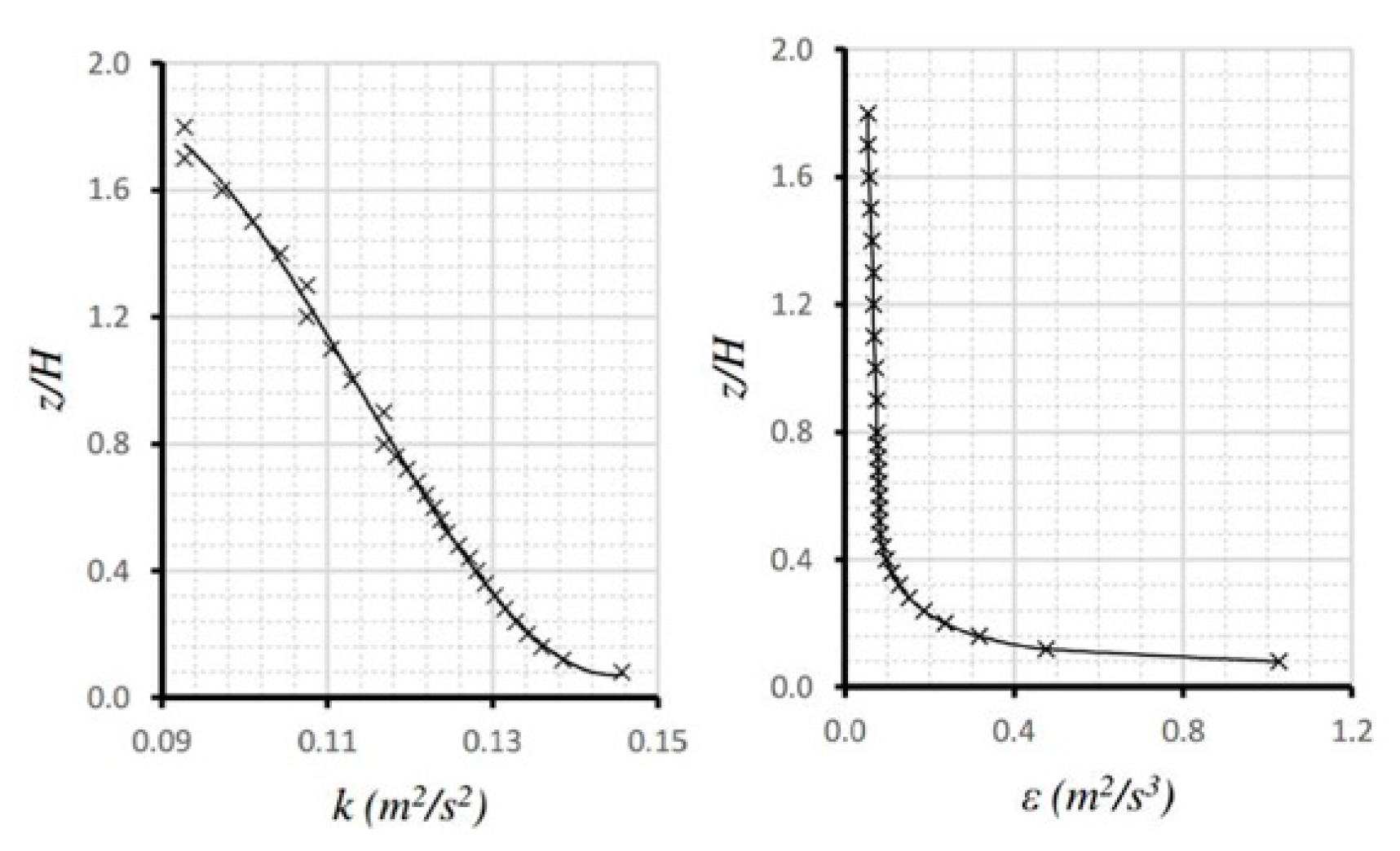
16]. The air supply (inlet) was simulated considering the dynamic characteristics of the wind and turbulence profiles acquired along the sub-urban flow. Equations (7)–(11) define the vertical profiles of wind velocity, turbulent kinetic energy and its dissipation [
26] (Equations (1)–(5)):
where
is the Von Karman constant (≈0.41),
the height,
the air mean velocity,
the air density (1204 kg/m
3 at 20 °C),
the height of the experimental domain,
the dynamic viscosity of the air (1.825 × 10
−5 N·s/m
2 at 20 °C) defined by the kinematic viscosity (
≈ 1.516 × 10
−5 m
2/s),
an empirical constant with an approximate value of 0.09 stated by Launder et al. (1974) [
27],
is the turbulent dynamic energy,
the turbulent energy near the walls and
the turbulent dissipation which are directly involved in air stagnation or short-circuiting air process.
The boundary conditions were defined according to the parameters of the scale model (
Table 1). Boundary conditions and aero-dynamical parameters for the simulation of the model (
Table 2) were stablished by the wind profiles, simulating the influence of the sub-urban environment in the building [
28].
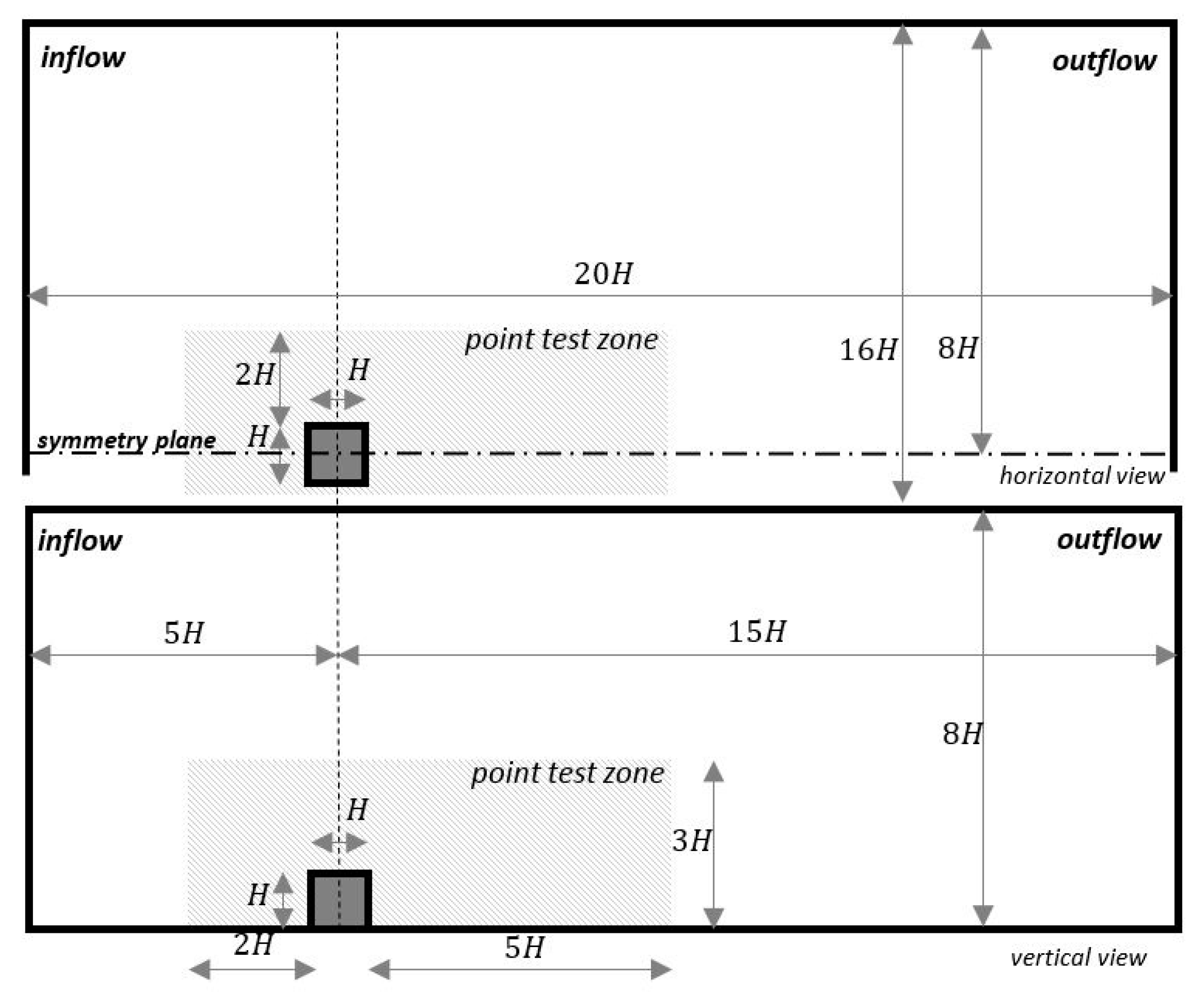
The complete definition of the cross section was required due to both the influence of the tunnel walls and the blocking effect implied by the built obstacle. The dimensions of the initial simulated domain reached a length of 20
H and a total width of 16
H, whose coordinate origin corresponded to the geometric centre of the cubic volume at the ground level. The dimensional requirements of the minimum lateral length, which must exceed 5
H, were satisfied [
16].
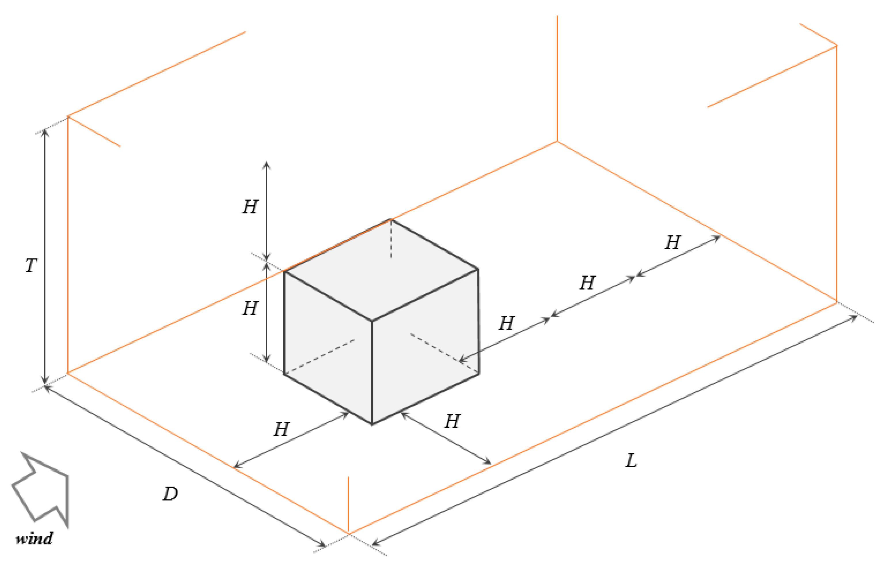
The sampling zone provided by the CEDVAL project covered the immediate surroundings of the cubic built volume to a maximum distance of 2
H, which is measured from the front, top and lateral sides of the volume (
Figure 1).
Three models of turbulence (Skε (standard-kε) [
27]; re-normalization group (RNG) [
29]; and realizable [
30]) were used to refine the simulated behaviour in the experimental results. Sequential simulations were carried out with two options for the wall effect assessment (standard wall functions (SWF) and enhanced wall treatment (EWT)) under a criterion of “Simple” resolution and spatial discretization based on a steady Green–Gauss node-based analysis.
2.3. Mesh Design
A symmetric hexahedral three-dimensional mesh was designed with a total of 2,430,456 cells and 926 nodes in line with the verification points provided for the pilot testing in the wind tunnel. The mesh is divided into two halves by a longitudinal plane of symmetry through the coordinate origin. The cells progressively reduced in size in relation to their proximity to the built volume, with a mean variation below 12%. The smaller cell size (2y) (Equation (6)) had a dimension of 0.05
H, which complied with the standard defined by the practice guideline for CFD [
25]. In this way, the cells which were located within the viscous sublayer of the computational model were affected by the logarithmic law of velocities.
where y is the centroid normal distance of the first cell in contact with the surface and
is the transverse stress of the fluid.
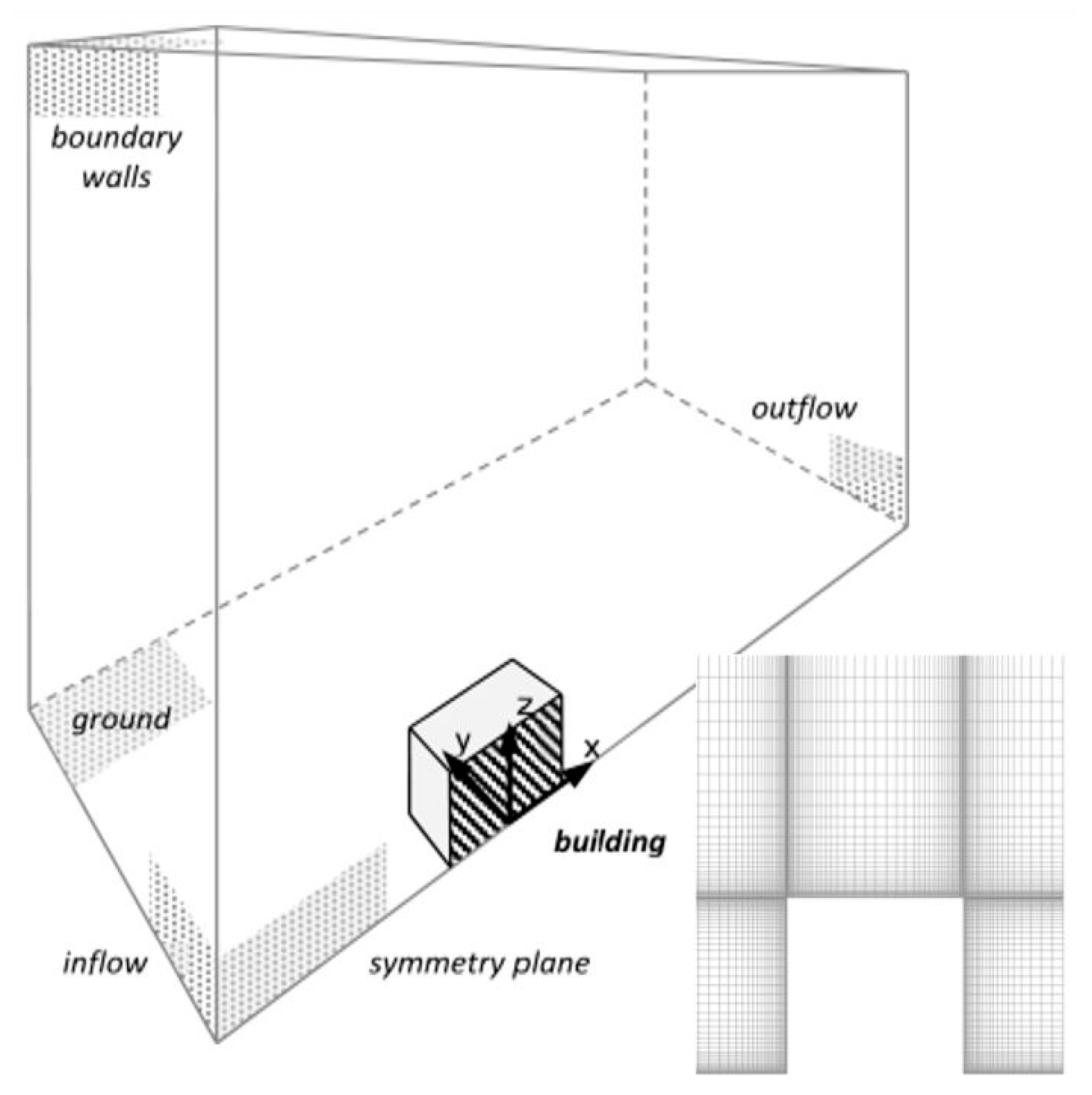
The boundary conditions for the wind tunnel surfaces were defined (
Figure 2). The inlet is provided through the front surface (inflow), by which the velocity and turbulence profiles are established. The outlet was performed by the rear surface (outflow), conditioning turbulence and flow equilibrium. Friction and shear stress conditions on the ground were uniformly defined [
31].
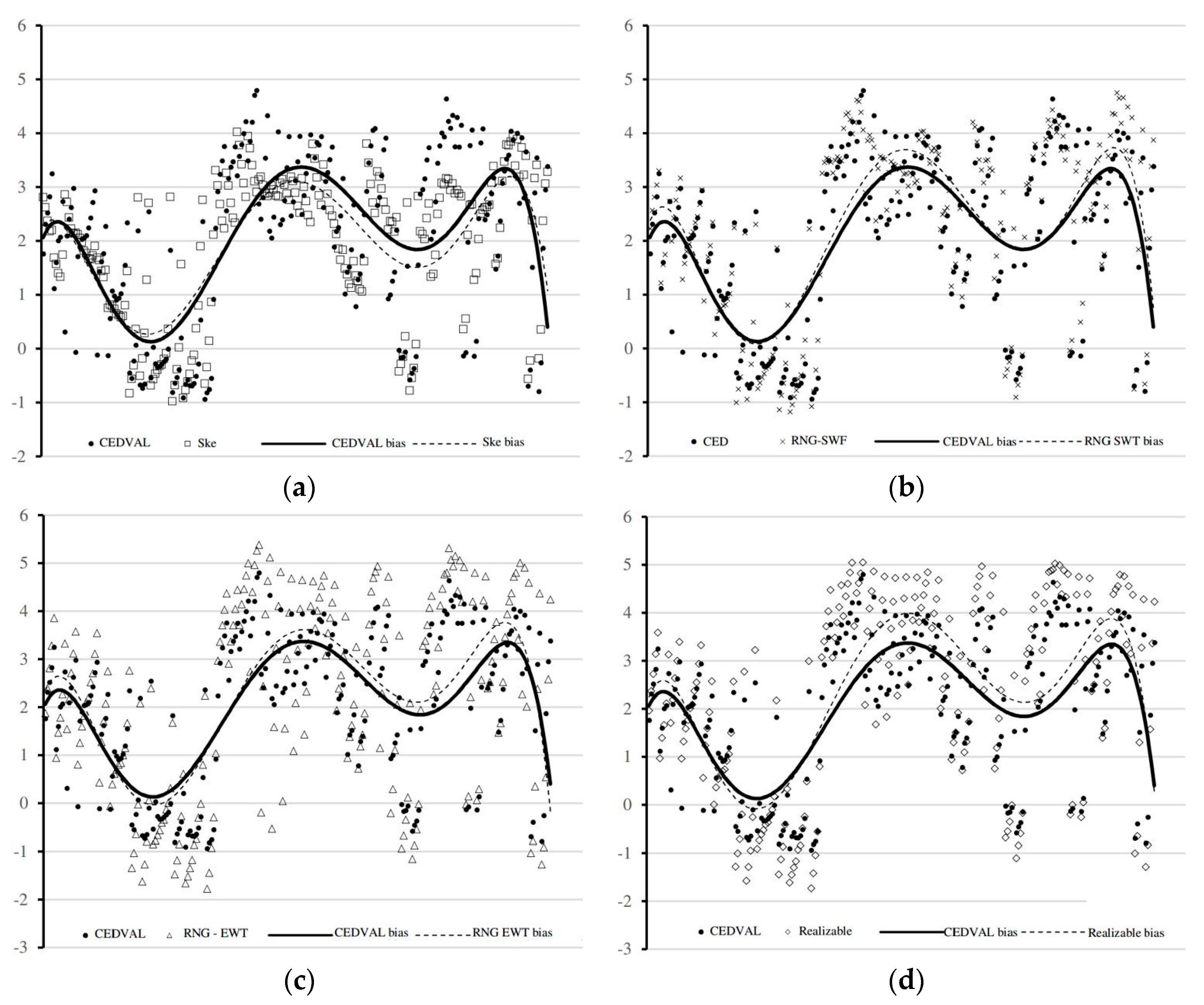
The accuracy of the mesh was evaluated by comparing the outcomes with those from CEDVAL (
Figure 3). The suitability of the mesh was verified for the analysed spatial discretization criteria by using measurement nodes (local mean deviation), reaching a mean deviation lower than 4% (mesh and setting criteria). The accuracy was estimated for all sampling points (
Table 3). It demonstrated a higher deviation in the points close to the cubic building and in the lower layers of the model (<0.1
H), both compared with the entire sample. This was due to the high turbulent energy that was generated. Local mean deviation remained over the maximum and commonly accepted deviation of 5% (realizable-EWT).
2.4. CFD Model Validation
CFD case A1–4 was validated from contrasting sources to verify previous statements [
24]. The realizable turbulence model (realizable-EWT) was the most accurate for the combined evaluation of the net velocity (velocity magnitude) and the predominant wind direction (X velocity) (
Table 3).
Measurements inside the wind tunnel provided characteristic horizontal velocity data, which were considered during the validation process. Horizontal velocity results provided the main characterization of the air behaviour in the vicinity of the building because of the kinetic turbulent energy and its dissipation capacity. Vertical and perpendicular components from the wind were rejected [
24], as they were established during the tests. Therefore, it was possible to check different turbulence models and to compare them with the processing times drop and the resulting data accuracy (
Figure 4).
The accuracy of the CFD configuration was achieved with the boundary conditions and the generated mesh quality (
Table 3 and
Figure 2). The flow balance was reached between the inlet surface within the simulated tunnel volume and the outlet surface. The values obtained were 6.9139185 kg/s at the inlet and −6.9138746 kg/s at the outlet, with a percent residual lower than 0.001%.
The surfaces which were directly exposed to the main wind component favoured the rise of turbulent airflows with higher intensity near the building volume. This phenomenon was caused by the increase of the shear stresses that occurs once the obstacle was overcome. The collision of air currents with the interposed obstacle altered the airflow components and generated a flow bifurcation and re-adherence to the solid surfaces that were pushed by the inertia forces, momentum and stresses. Vortex formation was observed. The results obtained in the model validation suggested the viability of the CFD model [
32], obtaining flow patterns which were similar to those obtained in the wind tunnel experiments.
2.5. Outdoor Air Change Quality and Efficiency
The turbulence effect on the air change quality relied on the vortices generated, which were more likely to produce air mass stagnation. The latter tends to occur in places where the dynamic action of the fluid is lower than the forces that promote the air change. This phenomenon is especially common in confined spaces where air is protected from the wind.
The air change efficiency concept refers to the quality of the process of exchanging the air with clean air. The mean age of the air (MAA) is the key concept by which the air change quality is evaluated [
33]. This concept consists of the characterization of the air flow particles inside a domain by evaluating the time they spend inside. Knowing the air flow used for ventilation and the volume of the domain, the calculation of the mean time which the air takes to complete the trajectory from the inlet to the outlet can be developed. The local mean age of the air (LMAA) concept has been used to define the quality of air change for known confined spaces such as indoor spaces [
34]. Its value is experimentally obtained by using two existing and valid methods [
11]. It is possible to apply it numerically on CFD through user defined functions (UDF).
However, LMAA has not been equally developed for outdoor spaces [
35] such as the urban built environment. This concept is difficult to be validated for outdoor spaces due to the reduced capacity of monitoring tracer gas in atmospheric open environments. Tracer gas techniques require high emission flow rates for their detection in open environments. Nevertheless, it is feasible in scale experiments like wind tunnels. CFD simulation allows the evaluation of LMAA in outdoor domains by incorporating wind tunnel boundary conditions as if it was an indoor space [
11,
12] (Equations (7)–(9)).
where
is the LMAA value,
the normalised LMAA,
the local concentration (kg/kg), ṁ the index of homogeneous emissions (for tracer gases),
the surface perpendicular to the flow vector components,
the flow that passes through boundary domain surfaces,
the free-flow horizontal wind speed and
the air volume in the domain.
The problem of assessing the age of the air in outdoor spaces relies on both the urban environment [
35] and the limits of the domain to be considered (CD). This problem was addressed by considering the urban domain (full volume inside the wind tunnel) as a known confined volume of air (full computational domain), which was used as a domain of reference.
The air in small CD (i.e., immediate surrounding of a building) posed a problem when evaluating its LMAA due to the blocking of the flow, erratically altering the trajectory of the air. The air flow balance was not distributed over regular inlet and outlet surfaces. It is necessary to determine where the air enters and exists the surfaces, defining the limits of the CD. Those boundaries were limited by the value at which the normal component of the flow contour was zero.
The polluted regions in an urban environment can be assessed by means of LMAA, which is directly related to the time the air takes to become charged with pollutants [
12]. This situation negatively affects the quality of the consumed air, which is influenced by the design-imposed characteristics of buildings [
36] and its ACH.
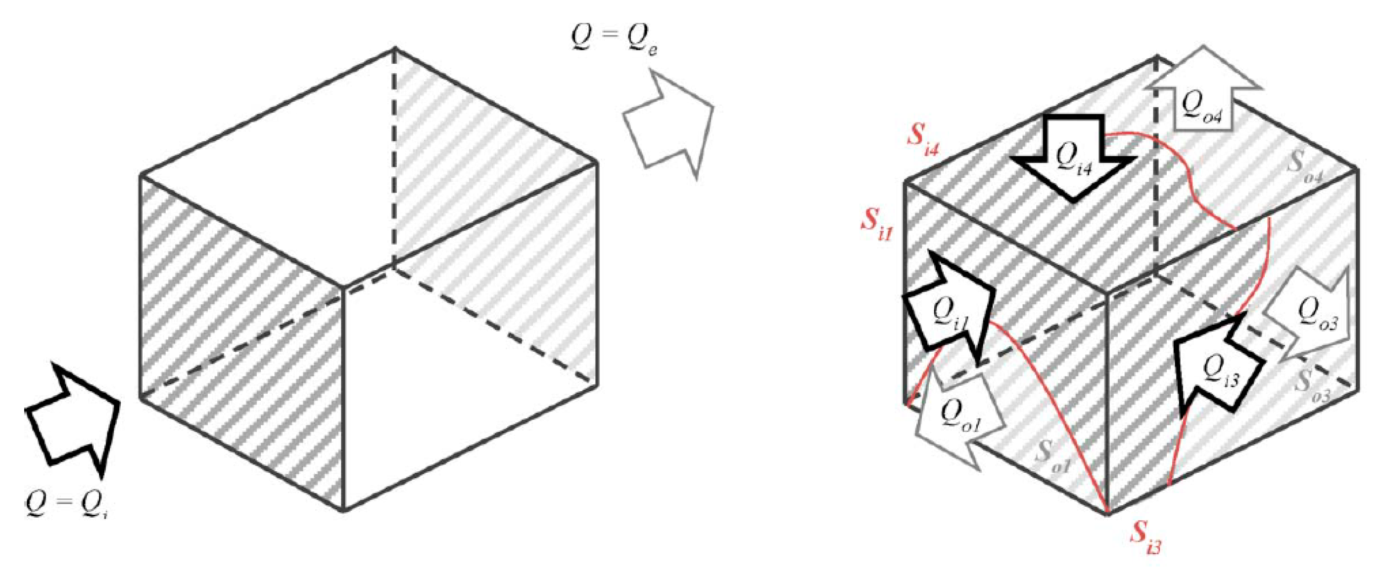
It is necessary to independently relate the air change quality from the chosen CD to evaluate the impact of the built environment in its global air quality. This was done by using the air change efficiency concept [
15]. The LMAA of the considered CD depends on the MAA at its boundary surfaces, through which the airflow enters and exits the domain (
Figure 5). The assessment of the mean residence time of the airflow particles was dimensionless, evaluated with regard to the time it would take if the obstacle did not exist and under ideal conditions (minimum residence time) (Equations (10)–(13)). It did not rely on the flow direction through the inlet and outlet surfaces.
where:
is the theoretical value for the output age of the air;
is the real output age of the air (residence time of the air in the CD) and
is the OACE.
This research aims to evaluate the impact of the considered CD in the outdoor air behaviour in order to define an ideal one: an ICD. The establishment of an ICD implies the simplification of the CFD simulation of dynamic outdoor air patterns for the evaluation of their quality. This influences our ability to analyse the outdoor conditions of the built environment with respect to the quality of life of the citizens and the optimization of the energy resources involved in the process of natural ventilation of buildings.
The OACE rate () is an objective index that depends on the size and relative position of the CD with respect to the building. The value of the LMAA differs. It is an objective temporal value obtained through physical parameters. It is consistent with the laws of correspondence or transfer of momentum, which are not influenced by the selected CD. Therefore, the OACE value is only useful for comparisons among different buildings dimensions and configurations into a constant urban model. The accuracy of the OACE value is concluded to be directly dependent on the ICD, whose definition method is the novelty of the work.
3. Results and Discussion
The resulting ICD was determined by the combined analysis of two factors: the behaviour of the air and OACE accuracy. It is assumed that an ICD must effectively represent the air behaviour and all of the aero-dynamical parameters that intervene in the OACH. An incorrect selection of the CD can misevaluate the affection of the aero-dynamical parameters, resulting in a poor and vague analysis of the numerical model. Extension of the CD and the relative position of the building inside it are the most important variables to be considered for the precise simulation of the case. The extension of the CD affects its air volume, which is supposed to have an important impact over the OACE index. In order to obtain a consolidated result that justifies the research, the behaviour of the air at the built environment was analysed, and different random CD in the range of [
16] were evaluated, as well as their influence on the OACE.
3.1. Analysis of the Dynamic Air Behaviour in the Built Environment
In order to obtain some reference values for the aero-dynamic parameters, a whole section of the wind tunnel has been evaluated, affording a full CD.
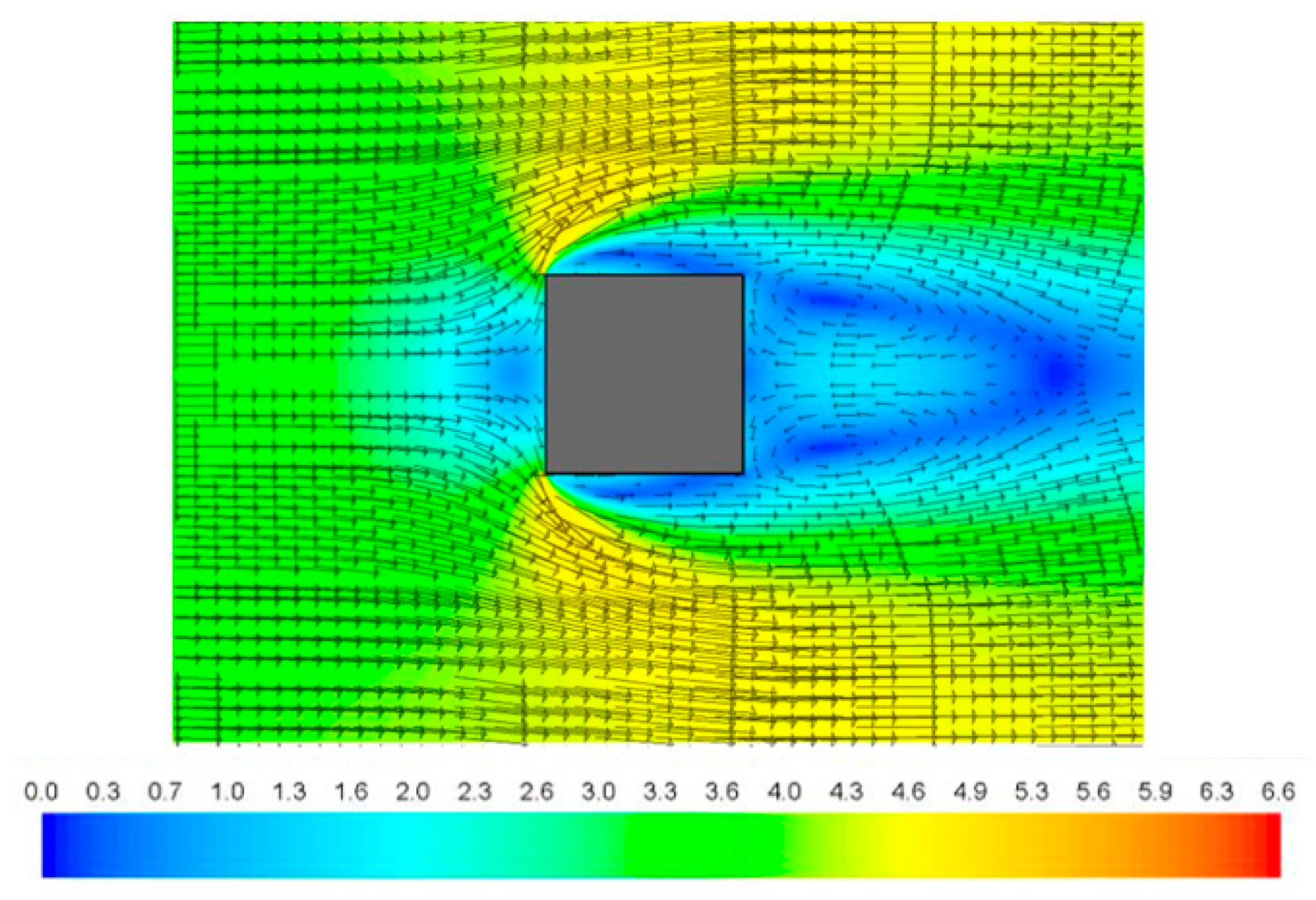
The airflow began to distort before reaching the building obstacle placed in between the normal wind flow at a distance
H from the front face (exposed to wind). Its impact continued downstream and a chaotic and irregular structure was retained beyond the limits of the simulated wind tunnel. The significant distortion effect of the airflow was developed at a distance of 5
H from the rear face of the obstacle (protected face). The internal forces and stresses generated before reaching the obstacle modified the upstream air particles’ motion pattern and created a “pressure bubble” facing the building (
Figure 6). It was observed approaching the building, in the vicinity of its front face and especially at the top front. Once the obstacle was overcome, the energy maintained a drag pattern which covered the building. It was graphically confirmed that these air regions of low turbulent energy had a higher age of the air than the rest of the domain, reducing its quality.
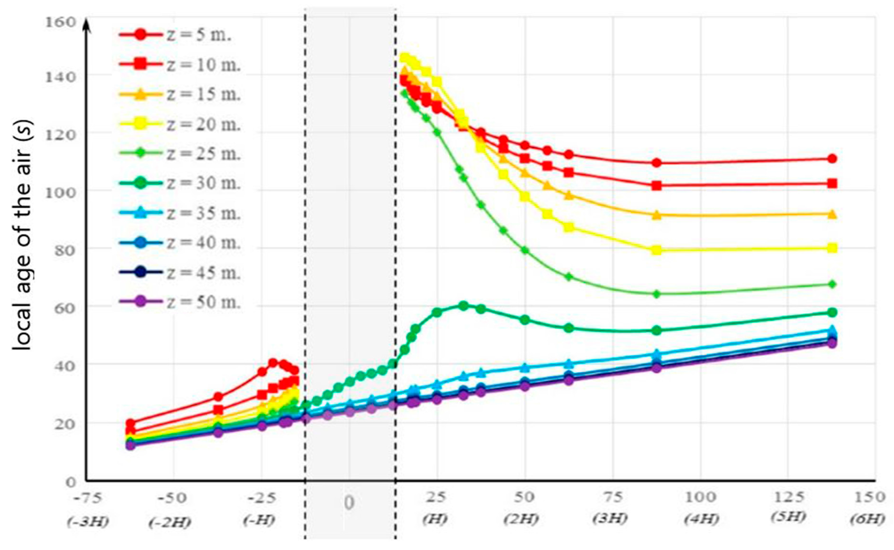
The creation of vortices is critical for the analysis of the air behaviour in the built environment due to the high Reynolds number (
Re ≈ 37.250) developed within the domain. Vortices appeared because of the alteration of the vector components acquired when the airflow was hampered [
37]. The turbulent vortices occurred where the turbulent energy decreased (turbulent dissipation growing). In a similar manner, the age of the air in an outdoor space is closely related to the air velocity, which reduces the air quality, increasing the LMAA (
Figure 7). This phenomenon does not affect the air change efficiency in the domain. It is confirmed that the results from the evaluation of the OACE depended on the extension of the CD.
3.2. ICD Determination
Some CD were defined in order to analyse the OACE and evaluate its accuracy. It volumetrically narrowed the limits of the study and assessed the patterns of the airflow behaviour around the building. This analysis was performed for several situations based on the air volume of the total wind tunnel (reference domain) by progressively varying the trapped air volume. It was necessary to define the inlet and outlet surfaces through which the air entered and exited the CD.
Minimum residence time of the air confined in the CD was obtained with the User Defined Function (UDF) specified for the age of the air evaluation applied to the CFD model. MAA was also evaluated for the CD air volume and at the outlet. OACE was obtained according to Equation (13).
The reference domain was evaluated considering the total air volume discarding the air volume corresponding to the building. An OACE value of approximately 100% (98.7%) was obtained (piston effect airflow model). This result was attributed to a low MAA, partially influenced by the obstruction. A significant proportion of the airflow crossed freely from the inlet to the outlet in the model without any building interference.
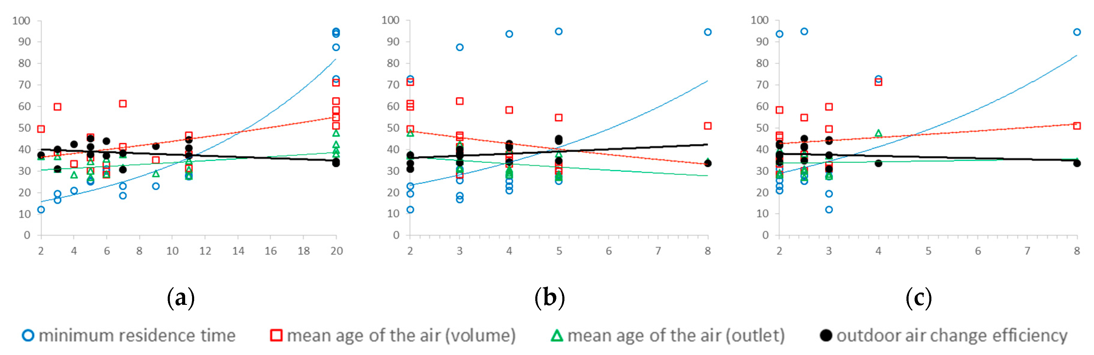
A total of 20 hexahedral extensions and proportions were analysed for the CD surrounding the building. The obtained results are analysed for each of the dimensional ranges (
Figure 8). The growth of any dimension of the CD resulted in the exponential increase of the minimum residence time. OACE remained practically stable with downward trend.
Table 4 shows the results that intervene in the accuracy of the OACE value. The minimum residence time is a theory-based number that represent the time the air change takes to fully exchange the air volume in the domain. The air volume depends on the volume of the selected CD minus the building volume that should be constant. The smaller the CD air volume is (the smallest possible dimension), the more effective is the computation process. The LMAA of the air volume contained in the CD should approximate the value obtained for the reference domain (first row). MAA value and outlet area affects the OACE index, which should be close to the mean value for all cases, except the reference value, which is for ideal situations.
The CD which best represented these requirements showed the highest accuracy of the LMAA, with similar air change times. The example which best exemplified the air behaviour and met the requirements imposed had the following dimensions: L = 5
H; D = 3
H and; T = 2
H (
Figure 9). The proposed ICD provided a LMAA value of the volume of 45.6 s, similar to the Reference Domain LMAA (45 s), with just 1% of the reference domain air volume. The mean OACE for the studied cases was 37.97%, with a tolerance of ±7.21%. The proposed ICD provided an efficiency of 37.75%, which had a value of −0.22%.
3.3. Discussion
The validation of the results obtained using the CFD numerical calculation method was performed with data provided by the Meteorological Institute of Universität Hamburg. The obtained airflow behaviour pattern was similar to the total behaviour of the scale model experimentally evaluated in the wind tunnel.
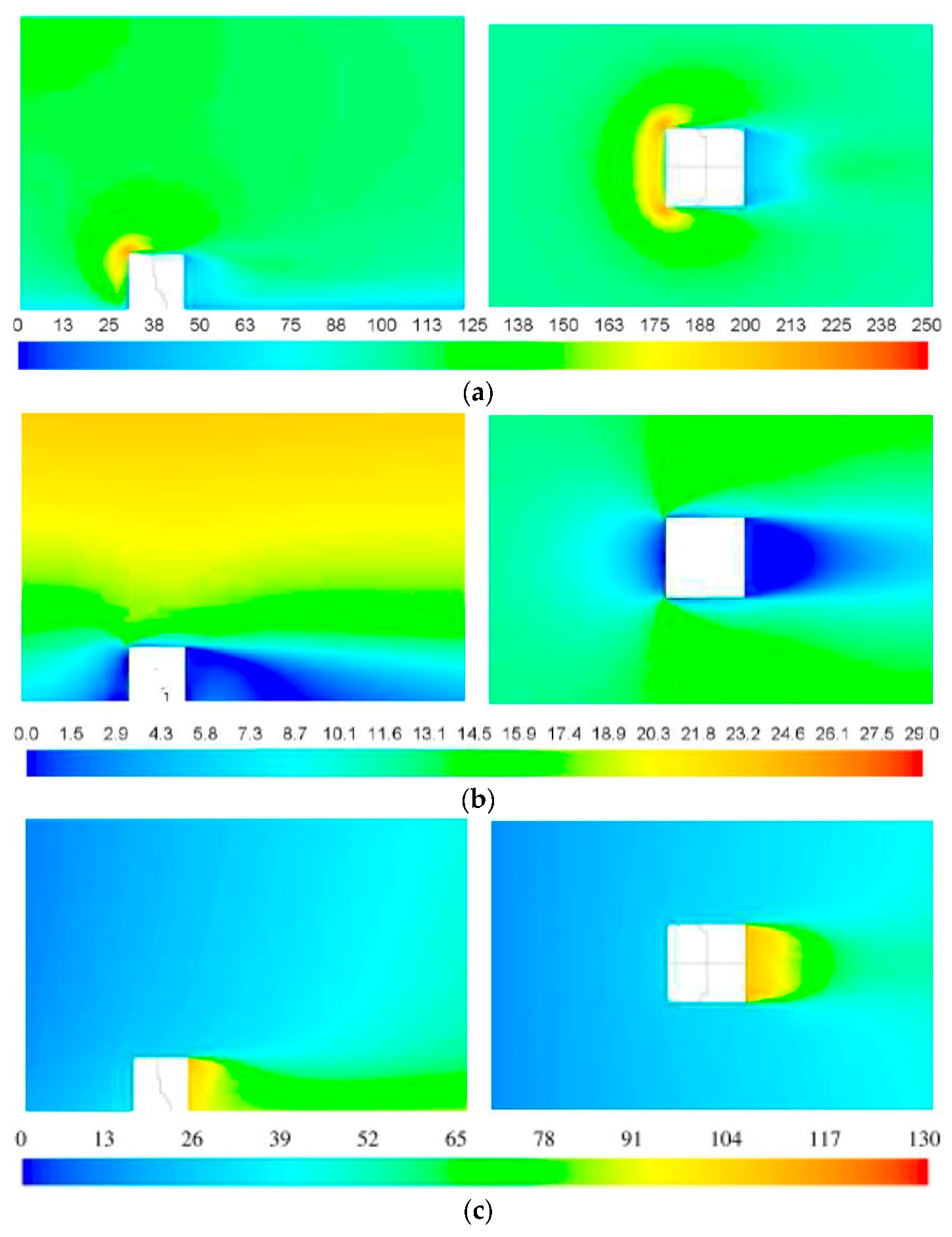
The methodology was conducted performing a double analysis. First, the outdoor air behaviour around a cubic-shaped building was analysed. These results are represented in
Figure 10. They demonstrate that the age of the outdoor air is related to the dynamic pressure and to the turbulence energy and its dissipation (
and
) in the wind tunnel.
It is verified that the air masses located in the lower parts of the model concentrate most of the urban pollutants due to their stagnation (higher age of the air), affecting its quality. Thus, the age of the air is lower in the higher points of the built volume exposed to the wind. Conversely, there is a confluence of dynamic effects at the lowest points of the built back surface, which is shielded from the wind, favouring the increase of contaminants concentration, which results in a progressive deterioration of the air quality [
38,
39,
40]. Subsequently, the ICD is assessed for the comparative evaluation of different architectural configurations in the same built environment. The proposed ICD includes the air that surrounds the building, where the dynamic phenomena that directly affect the outdoor air change occur. It has been extensively verified in previous studies [
3].
4. Conclusions
The air quality in the urban environment depends on both the level of pollution emissions and the urban mesh capacity, in order to favour their mixture with the air from rural and sub-urban areas. Its assessment is proposed through the concept of ventilation efficiency. The OACE has not been previously studied in depth due to the problems involved in the measurement of tracer gas concentration in open spaces, such as an urban environment.
A definition of an ICD is proposed to allow the evaluation of the OACE of any open environment through prior validated numerical simulation. The ICD allows the simplification of the evaluation procedure of the natural ventilation in buildings with outdoor air by studying behaviour patterns.
The dimensions of the ICD are proposed in relation to the dimensions of the analysed building structure and according to the results shown in
Table 4. In particular, this study examines the outdoor air change quality through the OACE index around a building that covers a minimum of 1
H in front of the exposed surface, above the cover and on the sides of the building enclosure. In addition, once the obstacle is overcome, the simulated volume coverage should be increased by a minimum length of 3
H from the rear surface, which is protected from the wind, since a significant degree of air stagnation is evident behind this surface. This finding demonstrates the consequent increase of the residence times of the air particles, which are promoted by both the low intensity of the dynamic pressure and the low turbulent intensity.
The accuracy of the OACE value is concluded to be directly dependent on the ICD, whose definition method is the novelty of the work.
Finally, the proposed ICD satisfies the requirements for the evaluation of the air behaviour in the built environment with an accuracy deviation lower than 0.58%. Results obtained in this research work will be used to formulate architectural design-based proposals to improve outdoor air change quality.


