
A New MCP Method of Wind Speed Temporal Interpolation and Extrapolation Considering Wind Speed Mixed Uncertainty

Abstract
:1. Introduction
2. Granular Computing Theory
3. Uncertainty Analysis of Wind Speed
3.1. Method for Calculating Uncertainty
3.2. Hierarchy of Uncertainty
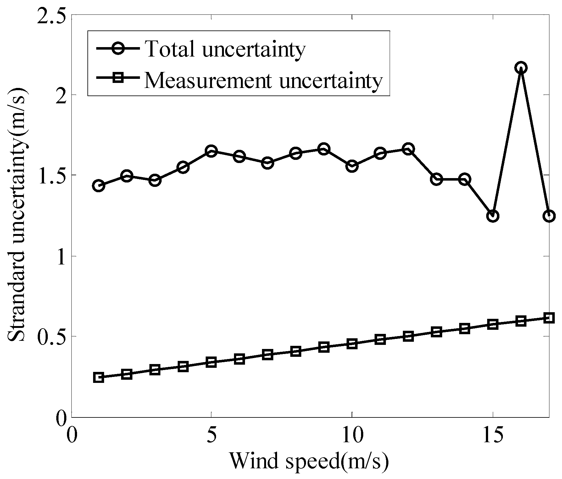
3.3. Uncertainty of Wind Speed Measurement
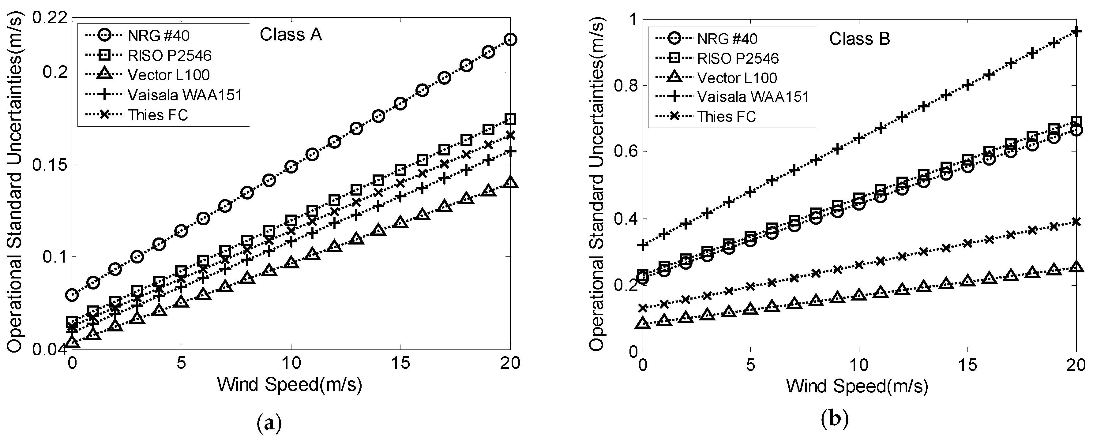
3.3.1. Operational Characteristics Uncertainty
3.3.2. Mounting Effects
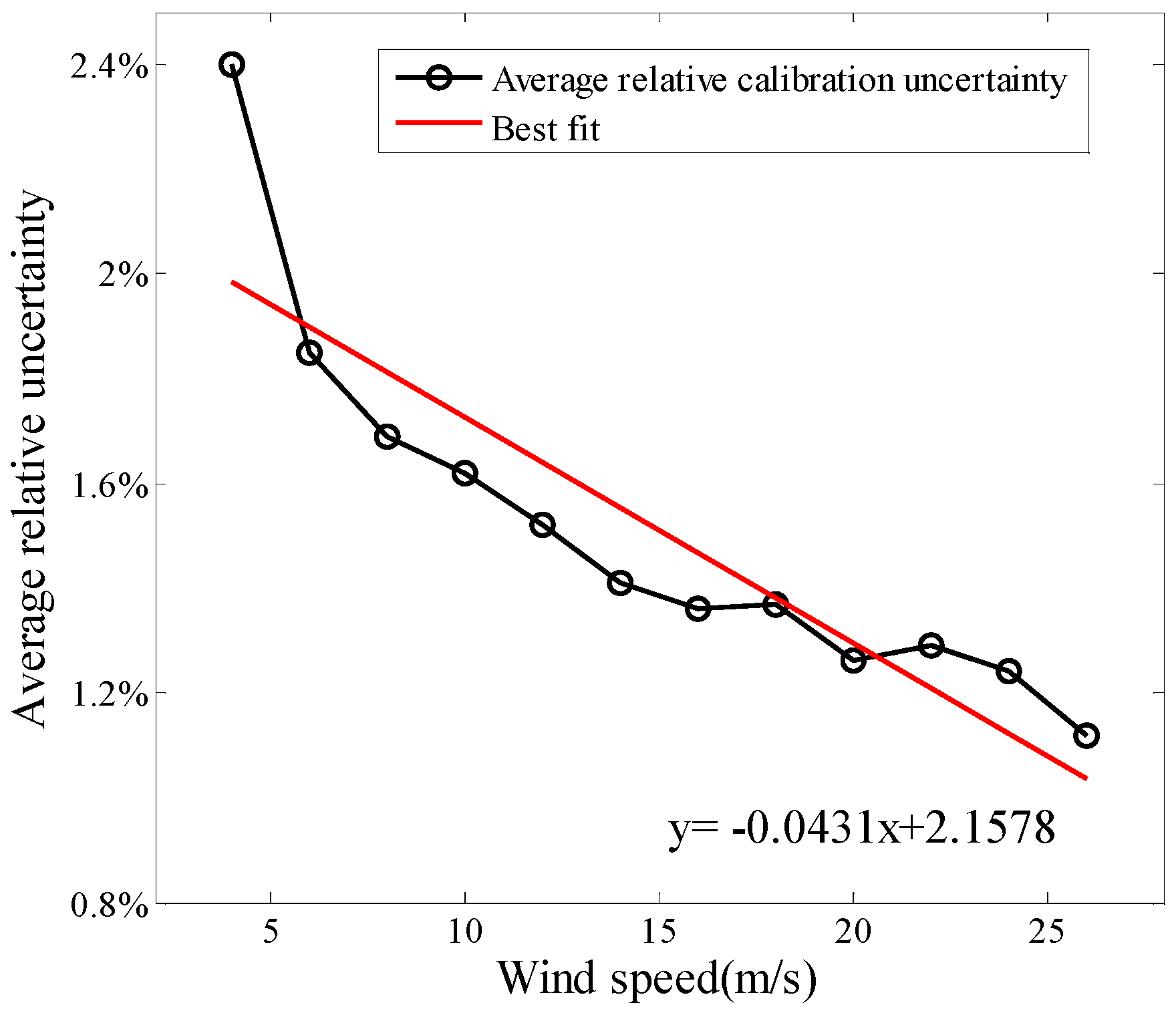
3.3.3. Uncertainty of the Anemometer Calibration
3.3.4. Uncertainty of Data Acquisition
3.3.5. Combined Uncertainty of Wind Speed Measurement
3.4. Combined Uncertainty
4. Proposed Method
4.1. Procedure of Proposed Method
4.2. Determining the Granular Hierarchy
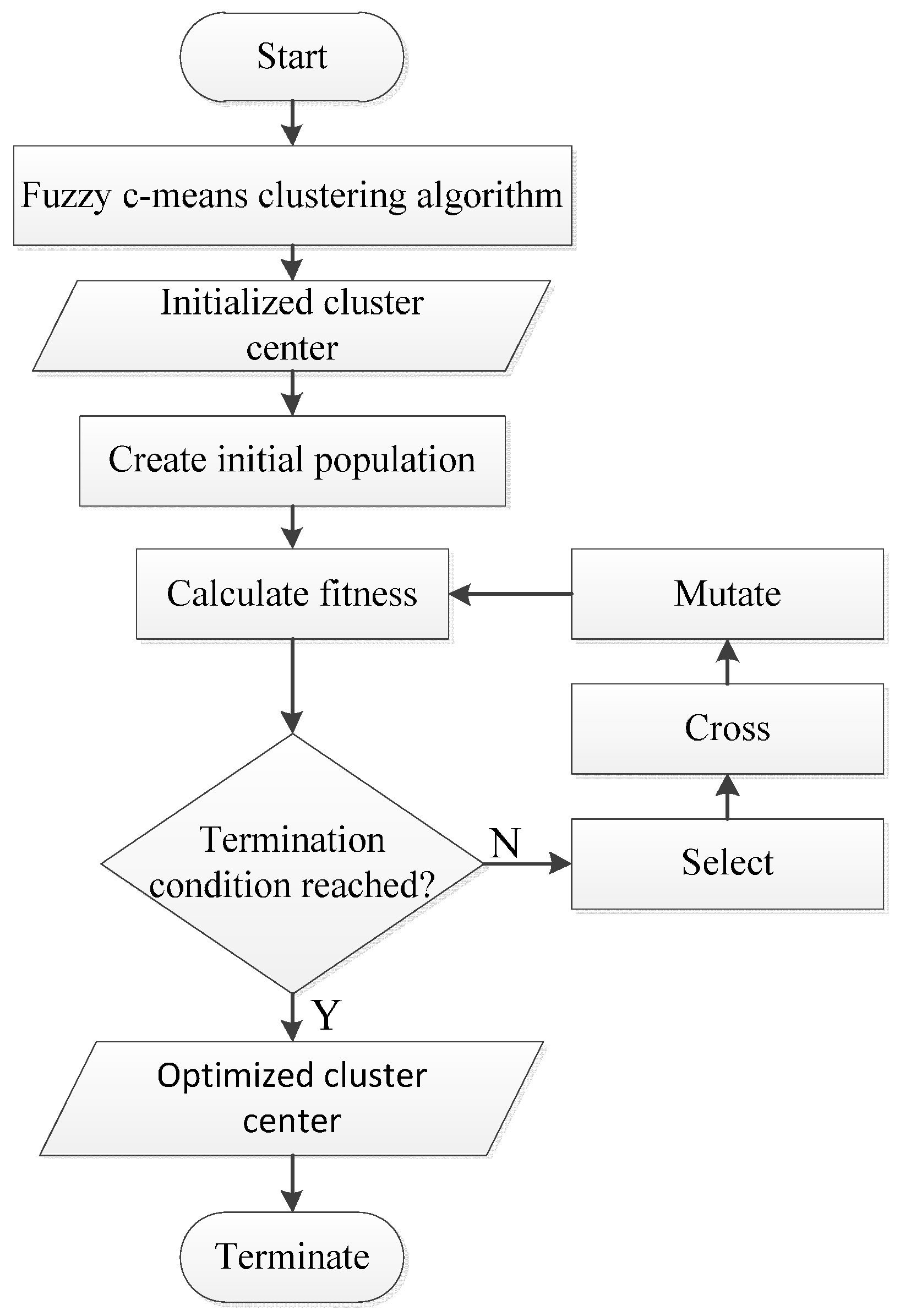
4.3. Granulation
- (a)
- Fix , , , . Choose an initial matrix . Then at step , ;
- (b)
- Compute means , = 1, 2, ...., with equation ; ;
- (c)
- Compute an updated membership matrix with equation ; ; ;
- (d)
- Compare to in any convenient matrix norm. If , stop. Otherwise set and return to Step (b).
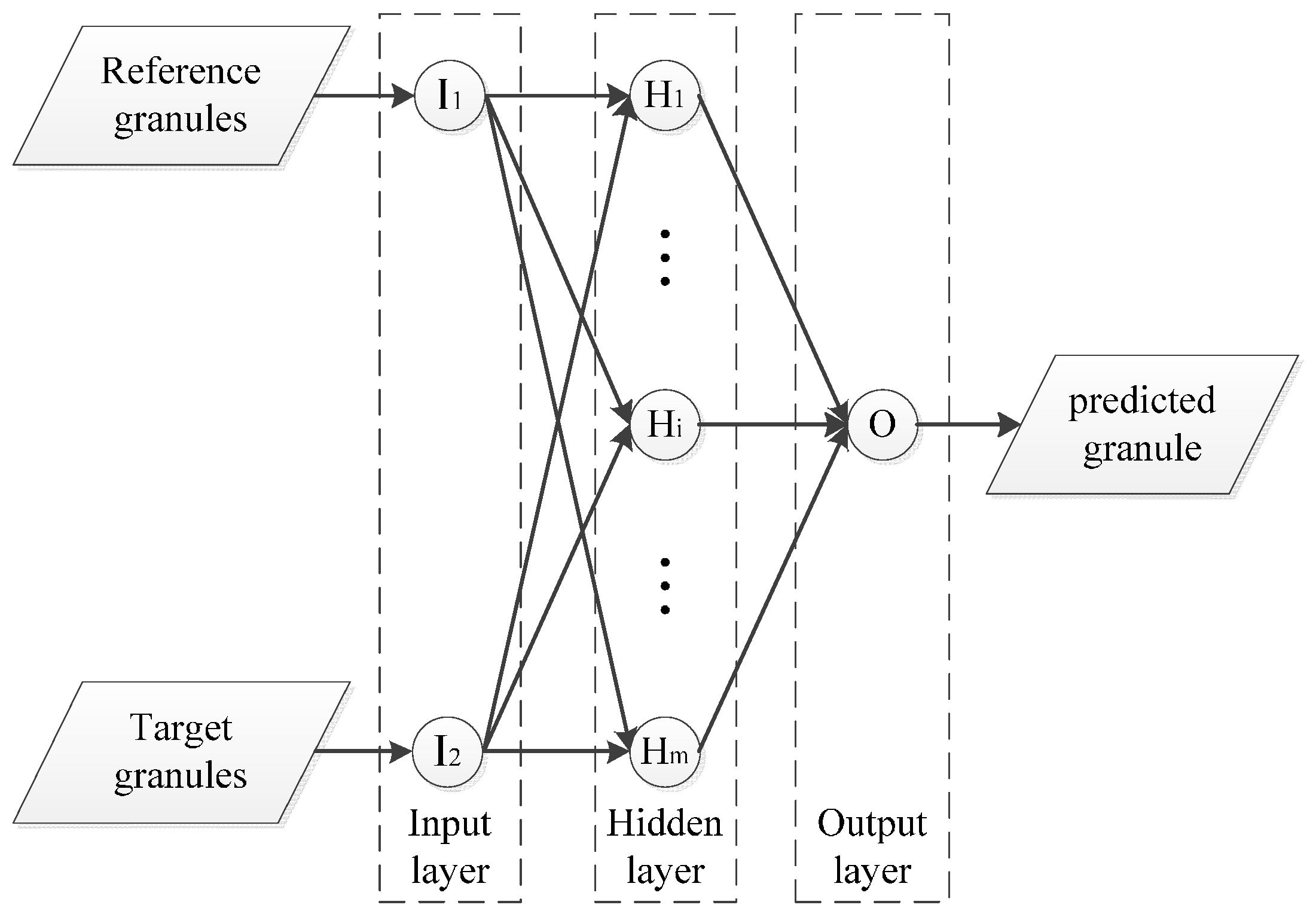
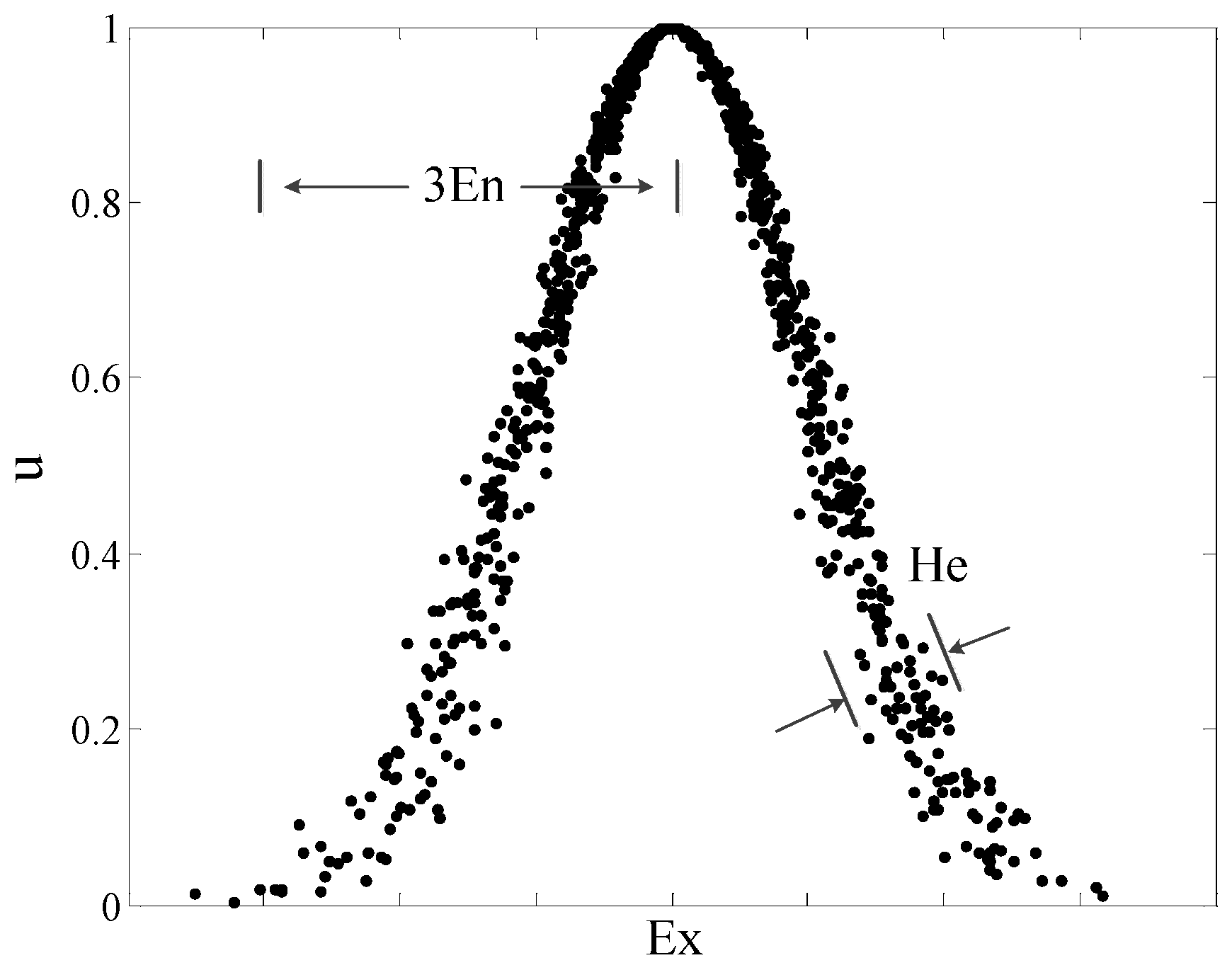
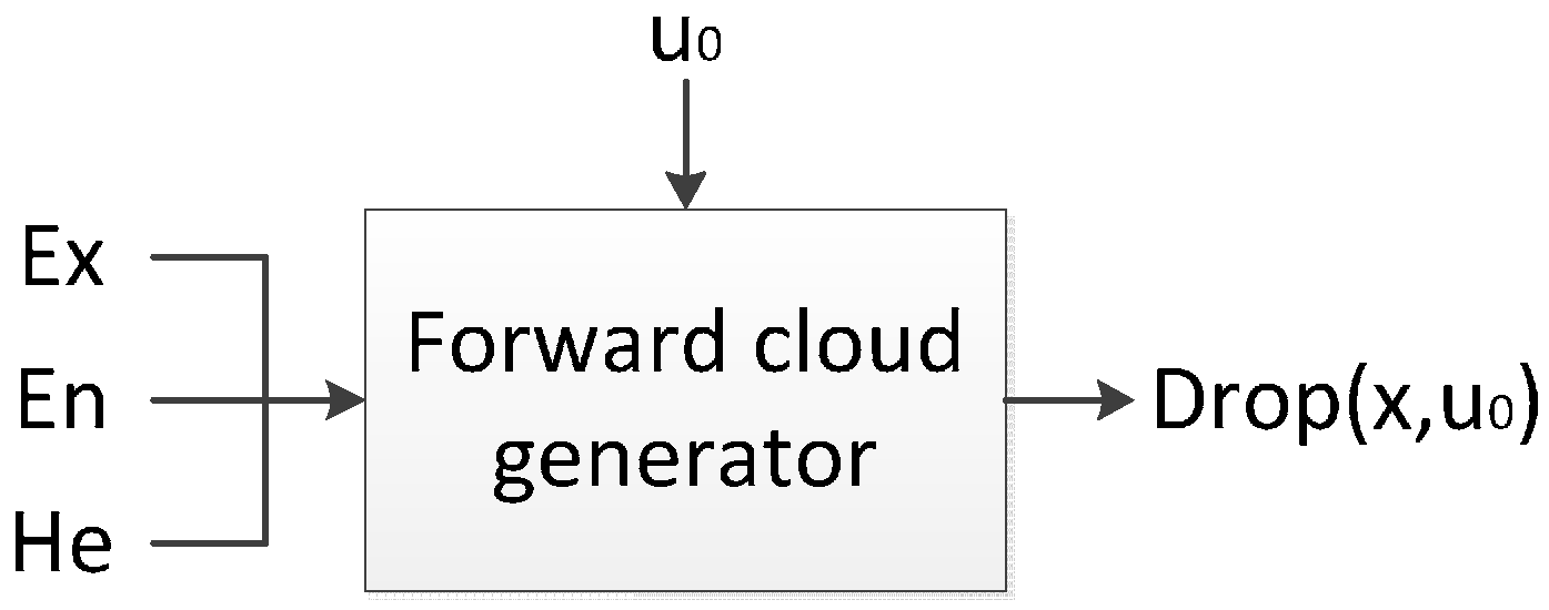
4.4. Granules Representation
4.5. Granular Computing
4.6. Interpolation and Extrapolation
5. Case Study
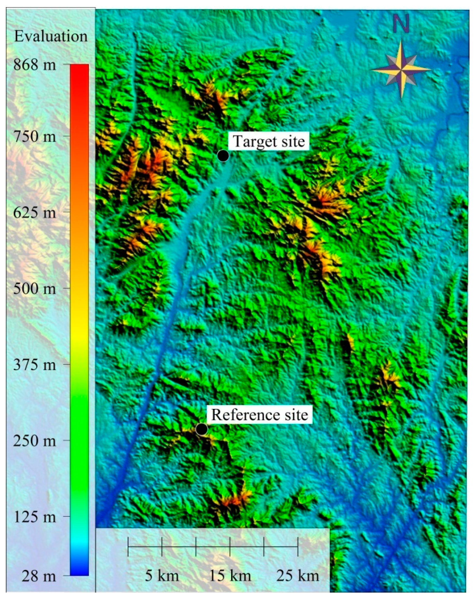
5.1. Case Study Description
5.2. EvaluationMetrics Used
5.3. Determining the Granular Hierarchy
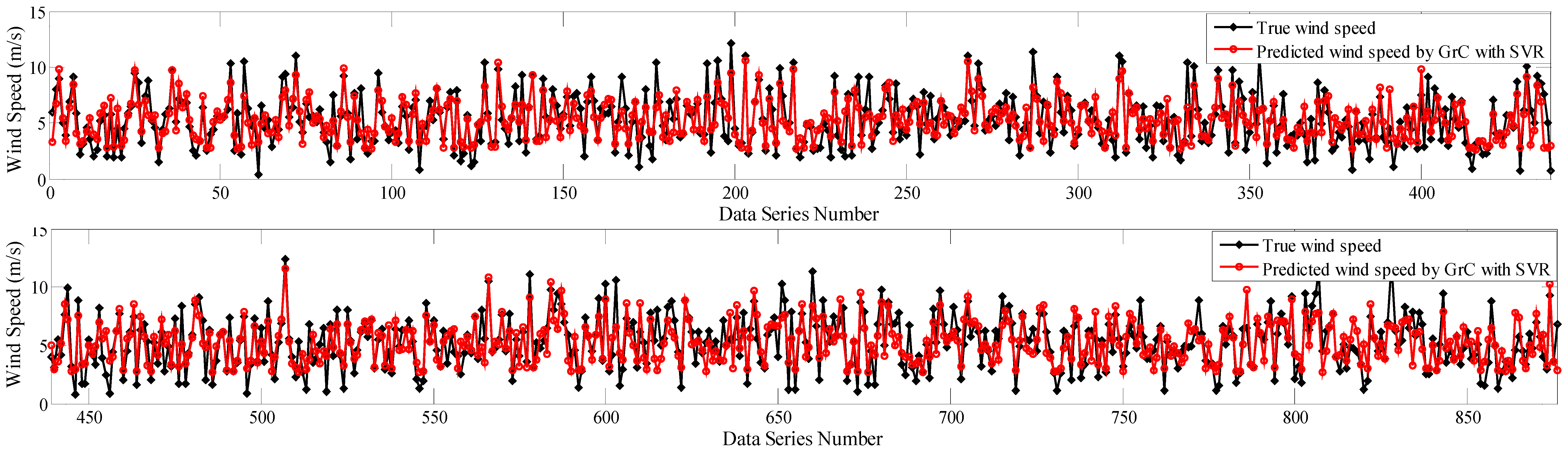
5.4. Results Analysis
6. Conclusions
- By using the MCP method proposed in this paper, mixed uncertainty of wind speed had already been considered, thus, a better estimation of the wind speed is provided compared to other methods selected for comparison. In the case study, almost evaluation metrics of interpolation with the proposed method were superior to other methods used in comparison. In comparison to the linear method, the correlation coefficient of the proposed method increased 8.48%, and the MRE, MREEP, and RMSE decreased 61.04%, 60.98% and 15.76%, respectively. The proposed method improved wind resource assessment accuracy and reduced the risks of wind farm construction.
- Suitability of using granular computing methods for the issue of wind speed data interpolation and extrapolation is proved. By using GrC method, wind speed mixed uncertainty can be taken into account; accurate results and low cost solutions can be derived.
- Mixed uncertainty of wind speed can be divided into three levels, and recommended values of granularity are minimum interval of records, 0.3–0.8 m/s, and 1–3 m/s, respectively. Also, estimation tools for wind speed measurement uncertainty and combined uncertainty are provided.
Acknowledgments
Author Contributions
Conflicts of Interest
References
- Burton, T.; Jenkins, N.; Sharpe, D.; Bossanyi, E. Wind Energy Handbook, 2nd ed.; John Wiley & Sons: Chichester, UK, 2011. [Google Scholar]
- European Wind Energy Association. Wind Energy-the Facts: A Guide to the Technology, Economics and Future of Wind Power; Earthscan: London, UK, 2009. [Google Scholar]
- Derrick, A. Development of the measure-correlate-predict strategy for site assessment. In European Community Wind Energy Conference, Proceedings of the 1993 International Conference, Lubeck-Travemunde, Germany, 8–12 March 1993; Garrad, A.D., Palz, W., Screller, S., Eds.; Stephens, H.S. and Associates: Bedford, UK, 1993; pp. 681–685. [Google Scholar]
- Ramsdell, J.V.; Houston, S.; Wegley, H.L. Measurement strategies for estimating long-term average wind speeds. Sol. Energy 1980, 25, 495–503. [Google Scholar] [CrossRef]
- Woods, J.C.; Watson, S.J. A new matrix method of predicting long-term wind roses with MCP. J. Wind Eng. Ind. Aerodyn. 1997, 66, 85–94. [Google Scholar] [CrossRef]
- Lackner, M.A.; Rogers, A.L.; Manwell, J.F. Uncertainty analysis in MCP-based wind resource assessment and energy production estimation. J. Sol. Energy Eng. 2008, 130. [Google Scholar] [CrossRef]
- Thøgersen, M.L.; Nielsen, P.; Sørensen, T.; Svenningsen, L.U. An Introduction to the MCP Facilities in WindPRO. EMD International A/S, 2010. Available online: http:/help.emd.dk/knowledgebase/content/ReferenceManual/MCP.pdf (accessed on 17 June 2017).
- Khadem, S.K.; Hussain, M. A pre-feasibility study of wind resources in Kutubdia Island, Bangladesh. Renew. Energy 2006, 31, 2329–2341. [Google Scholar] [CrossRef]
- Abbes, M.; Belhadj, J. Wind resource estimation and wind park design in El-Kef region, Tunisia. Energy 2012, 40, 348–357. [Google Scholar] [CrossRef]
- Mohandes, M.A.; Halawani, T.O.; Rehman, S.; Hussain, A.A. Support vector machines for wind speed prediction. Renew. Energy 2004, 29, 939–947. [Google Scholar] [CrossRef]
- Ji, G.-R.; Han, P.; Zhai, Y.-J. Wind speed forecasting based on support vector machine with forecasting error estimation. In Proceedings of the 6th International Conference on Machine Learning and Cybernetics, Hong Kong, China, 19–22 August 2007; pp. 2735–2739. [Google Scholar]
- Velázquez, S.; Carta, J.A.; Matías, J.M. Comparison between ANNs and linear MCP algorithms in the long-term estimation of the cost per kWh produced by a wind turbine at a candidate site: A case study in the Canary Islands. Appl. Energy 2011, 88, 3869–3881. [Google Scholar] [CrossRef]
- Addison, J.F.; Hunter, A.; Bass, J.; Rebbeck, M. A neural network version of the measure–correlate–predict algorithm for estimating wind energy yield. In Proceedings of the 13th International Congress and Exhibition on Condition Monitoring and Diagnostic Engineering Management, Houston, TX, USA, 3–8 December 2000; pp. 917–922. [Google Scholar]
- Saavedra-Moreno, B.; Salcedo-Sanz, S.; Carro-Calvo, L.; Gascon-Moreno, J.; Jimenez-Fernandez, S.; Prieto, L. Very fast training neural-computation techniques for real measure-correlate-predict wind operations in wind farms. J. Wind Eng. Ind. Aerodyn. 2013, 116, 49–60. [Google Scholar] [CrossRef]
- Liu, X.; Lai, X.; Zheng, F. Analysis of the interpolation method for wind speed data based on Reanalysis data. J. Huazhong Univ. Sci. Technol. 2017, 45, 78–83. [Google Scholar]
- Carta, J.A.; Velázquez, S. A new probabilistic method to estimate the long-term wind speed characteristics at a potential wind energy conversion site. Energy 2011, 36, 2671–2685. [Google Scholar] [CrossRef]
- García-Rojo, R. Algorithm for the estimation of the long-term wind climate at a meteorological mast using a joint probabilistic approach. Wind Eng. 2004, 28, 213–223. [Google Scholar] [CrossRef]
- Angelis-Dimakis, A.; Biberacher, M.; Dominguez, J.; Fiorese, G.; Gadocha, S.; Gnansounou, E.; Guariso, G.; Kartalidis, A.; Panichelli, L.; Pinedo, I.; et al. Methods and tools to evaluate the availability of renewable energy sources. Renew. Sustain. Energy Rev. 2011, 15, 1182–1200. [Google Scholar] [CrossRef]
- Bowen, A.J.; Mortensen, N.G. Exploring the limits of WAsP the wind atlas analysis and application program. In Proceedings of the 1996 European Wind Energy Conference and Exhibition, Goteborg, Swenden, 20–24 May 1996; pp. 584–587. [Google Scholar]
- Landberg, L.; Mortensen, N.G. A comparison of physical and statistical methodsfor estimating the wind resource at a site. In Proceedings of the 15th British Wind Energy Association Conference, York, UK, 6–8 October 1993; Pitcher, K.F., Ed.; Mechanical Engineering Publications Ltd.: London, UK, 1993; pp. 119–125. [Google Scholar]
- Yao, Y. Perspectives of granular computing. In Proceedings of the 2005 IEEE International Conference on Granular Computing, Beijing, China, 25–27 July 2005. [Google Scholar]
- Zadeh, L.A. Toward a theory of fuzzy information granulation and its centrality in human reasoning and fuzzy logic. Fuzzy Sets Syst. 1997, 90, 111–127. [Google Scholar] [CrossRef]
- Bargiela, A.; Pedrycz, W. Granular Computing: An Introduction; Springer Science & Business Media: New York, NY, USA, 2003. [Google Scholar]
- Lin, T.Y.; Yao, Y.Y.; Zadeh, L.A. Data Mining, Rough Sets and Granular Computing; Springer: Berlin, Germany, 2002. [Google Scholar]
- Zadeh, L.A. Some reflections on soft computing, granular computing and their roles in the conception, design and utilization of information/intelligent systems. In Soft Computing—A Fusion of Foundations, Methodologies and Applications; Springer-Verlag: Berlin, Germany, 1998; Volume 2, pp. 23–25. [Google Scholar]
- International Organization for Standardization. Uncertainty of Measurement—Part 3: Guide to the Expression of Uncertainty in Measurement; ISO: Geneva, Switzerland, 2008. [Google Scholar]
- International Electrotechnical Commission. Wind Turbines—Part 12-1: Power Performance Measurements of Electricity Producing Wind Turbines; IEC: Geneva, Switzerland, 2012. [Google Scholar]
- Risø National Laboratory. ACCUWIND—Classification of Five Cup Anemometers According to IEC61400-12-1. Available online: http://orbit.dtu.dk/fedora/objects/orbit:88359/datastreams/file_7703253/content (accessed on 17 June 2017).
- Coquilla, R.V.; Obermeier, J. Calibration uncertainty comparisons between various anemometers. In Proceedings of the American Wind Energy Association Wind Power Conference, Houston, TX, USA, 10 July 2008. [Google Scholar]
- Pal, N.R.; Bezdek, J.C. On cluster validity for the fuzzy c-means model. IEEE Trans. Fuzzy Syst. 1995, 3, 370–379. [Google Scholar] [CrossRef]
- Bezdek, J.C.; Ehrlich, R.; Full, W. FCM: The fuzzy c-means clustering algorithm. Comput. Geosci. 1984, 10, 191–203. [Google Scholar] [CrossRef]
- Scheunders, P. A genetic c-means clustering algorithm applied to color image quantization. Pattern Recognit. 1997, 30, 859–866. [Google Scholar] [CrossRef]
- Alata, M.; Molhim, M.; Ramini, A. Optimizing of Fuzzy C-Means Clustering Algorithm Using GA. World Acad. Sci. Eng. Technol. 2008, 2, 670–675. [Google Scholar]
- Li, D.Y.; Meng, H.J.; Shi, X.M. Membership clouds and membership cloud generators. J. Comput. Res. Dev. 1995, 32, 15–20. [Google Scholar]
- Di, K.; Li, D.R.; Li, D.Y. Cloud theory and its applications in spatial data mining and knowledge discovery. J. Image Graph. 1999, 4, 930–935. [Google Scholar]
- Li, D.Y.; Du, Y. Artificial Intelligence with Uncertainty; CRC Press: Boca Raton, FL, USA, 2017. [Google Scholar]
- Vapnik, V. The Nature of Statistical Learning Theory; Springer Science & Business Media: Dordrecht, The Netherlands, 2013. [Google Scholar]
- Nrgsystems. #40C Anemometer Uncertainty. Available online: https://www.nrgsystems.com/assets/resources/40C-Anemometer-Uncertainty-AppNote.pdf (accessed on 17 June 2017).


| Classification Category | Class A Ideal Flat Terrain Sites | Class B Non-Ideal Complex Terrain Sites | ||
|---|---|---|---|---|
| min | max | min | max | |
| Wind Speed Range (m/s) | 4 | 16 | 4 | 16 |
| Turbulence Intensity | 0.03 | 0.12 + 0.48/V | 0.03 | 0.12 + 0.96/V |
| Turbulence Structure () | 1/0.8/0.5 | 1/1/1 | ||
| Air Temperature (°C) | 0 | 40 | −10 | 40 |
| Air Density (kg/m3) | 0.9 | 1.35 | 0.9 | 1.35 |
| Average flow inclination (°) | −3 | 3 | −15 | 15 |
| Cup Anemometer | Classification Number | |
|---|---|---|
| Class A | Class B | |
| NRG #40 | 2.4 | 7.7 |
| RISO P2546 | 1.9 | 8.0 |
| Thies FC | 1.5 | 2.9 |
| Vaisala WAA151 | 1.7 | 11.1 |
| Vector L100 | 1.8 | 4.5 |
| Type of Anemometer | Relative Calibration Uncertainties of Anemometer Calibration | |||||||||||
|---|---|---|---|---|---|---|---|---|---|---|---|---|
| 4 m/s | 6 m/s | 8 m/s | 10 m/s | 12 m/s | 14 m/s | 16 m/s | 18 m/s | 20 m/s | 22 m/s | 24 m/s | 26 m/s | |
| NRG #40 | 2.65% | 2.00% | 1.62% | 1.49% | 1.45% | 1.43% | 1.38% | 1.23% | 1.08% | 1.43% | 1.03% | 0.90% |
| NRG IF3 | 4.04% | 2.74% | 1.98% | 1.81% | 1.57% | 1.40% | 1.18% | 1.12% | 1.10% | 1.01% | 1.07% | 0.90% |
| Risoe cup | 2.15% | 1.88% | 2.00% | 1.53% | 1.34% | 1.29% | 1.25% | 1.29% | 1.19% | 1.10% | 1.04% | 1.11% |
| R.M Young Wind Monitor | 1.47% | 1.05% | 0.84% | 0.76% | 0.68% | 0.64% | 0.61% | 0.60% | 0.60% | 0.61% | 0.58% | 0.58% |
| R.M Young Wind Sentry | 1.53% | 1.06% | 1.03% | 1.02% | 1.08% | 1.02% | 0.95% | 0.94% | 0.84% | 0.90% | 0.84% | 0.99% |
| Second Wind C3 | 2.74% | 2.19% | 2.14% | 1.66% | 1.60% | 1.47% | 1.51% | 1.45% | 1.34% | 1.31% | 1.09% | 1.00% |
| Thies First Class | 2.71% | 2.24% | 1.83% | 2.70% | 2.29% | 1.74% | 1.87% | 2.21% | 1.73% | 1.82% | 1.76% | 1.58% |
| Vaisala WAA252 | 2.70% | 2.04% | 1.90% | 1.87% | 2.07% | 1.89% | 1.80% | 1.92% | 2.05% | 1.84% | 1.86% | 1.68% |
| Vector V100LK | 2.46% | 2.13% | 2.22% | 2.27% | 2.04% | 2.02% | 1.92% | 2.01% | 1.83% | 2.03% | 2.15% | 1.66% |
| Vestas Cup | 1.50% | 1.19% | 1.35% | 1.10% | 1.12% | 1.20% | 1.14% | 0.96% | 0.83% | 0.85% | 1.00% | 0.78% |
| average relative uncertainties | 2.40% | 1.85% | 1.69% | 1.62% | 1.52% | 1.41% | 1.36% | 1.37% | 1.26% | 1.29% | 1.24% | 1.12% |
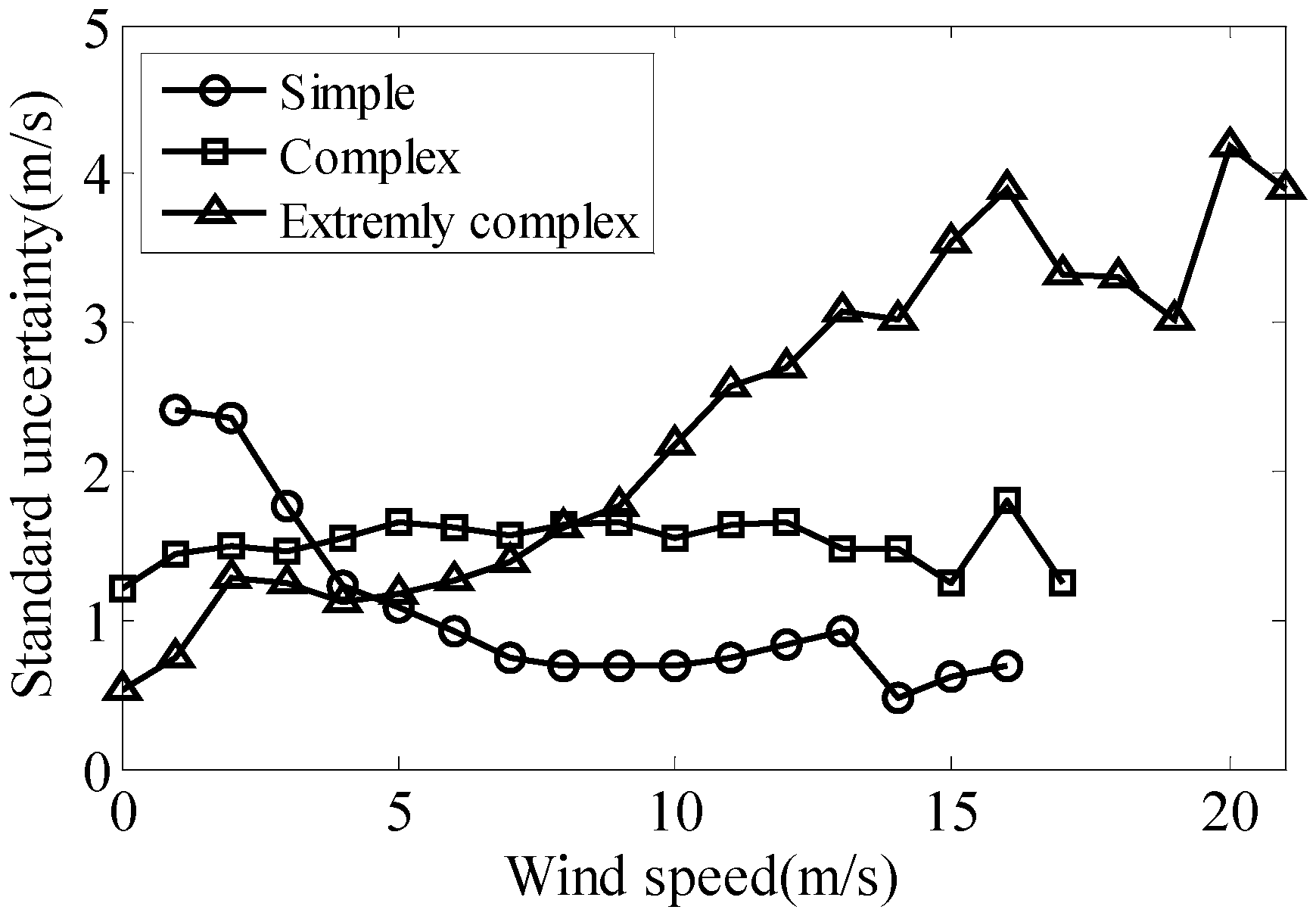
| Groups | Topography | Vegetation | Distance (km) | Correlation Coefficient |
|---|---|---|---|---|
| simple | plane | grass/crops | 8 | 0.793 |
| complex | hill | forest | 40 | 0.733 |
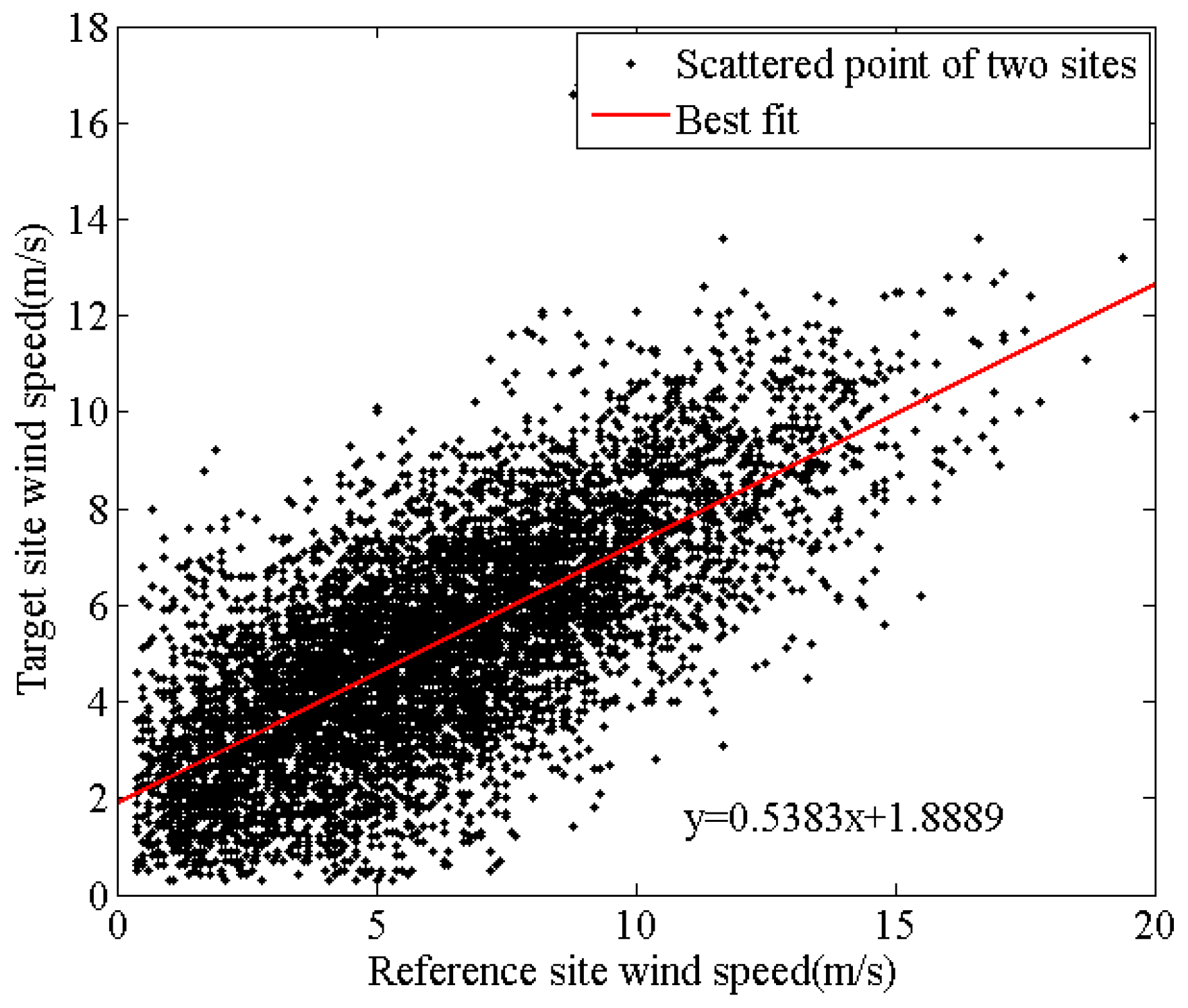
| extremely complex | mountain | forest | 15 | 0.872 |
| Parameters | Reference Site | Target Site |
|---|---|---|
| Location Elevation (m) | 620 | 430 |
| Local terrain | mountain | hill |
| Start date | 2012/1/1 | 2012/1/1 |
| End date | 2012/12/31 | 2012/12/31 |
| Anemometer type | NRG 40C | NRG 40C |
| Mounting height (m) | 70/60/50/30/10 | 70/60/50/30/10 |
| Evaluation Index | Linear Regression Method | Variance Ratio Method | ANN | SVR | Granular Computing Method with ANN | Granular Computing Method with SVR | ||||||
|---|---|---|---|---|---|---|---|---|---|---|---|---|
| Top | Middle | Bottom | Synthesized | Top | Middle | Bottom | Synthesized | |||||
| Level | Level | Level | Level | Level | Level | |||||||
| MRE | −0.77% | −2.01% | −1.42% | −1.37% | −1.75% | −0.85% | −1.42% | −0.32% | −1.19% | −0.79% | −1.37% | −0.30% |
| r | 0.731 | 0.732 | 0.779 | 0.782 | 0.752 | 0.745 | 0.779 | 0.789 | 0.768 | 0.757 | 0.782 | 0.793 |
| MREEP | −8.97% | 3.46% | −5.95% | −4.93% | −8.93% | −4.61% | −5.95% | −3.51% | −6.87% | −3.18% | −4.93% | −3.50% |
| RMSE (m/s) | 1.65 | 1.76 | 1.5 | 1.47 | 1.59 | 1.61 | 1.5 | 1.43 | 1.63 | 1.53 | 1.47 | 1.39 |
© 2017 by the authors. Licensee MDPI, Basel, Switzerland. This article is an open access article distributed under the terms and conditions of the Creative Commons Attribution (CC BY) license (http://creativecommons.org/licenses/by/4.0/).
Share and Cite
Liu, X.; Lai, X.; Zou, J. A New MCP Method of Wind Speed Temporal Interpolation and Extrapolation Considering Wind Speed Mixed Uncertainty. Energies 2017, 10, 1231. https://doi.org/10.3390/en10081231
Liu X, Lai X, Zou J. A New MCP Method of Wind Speed Temporal Interpolation and Extrapolation Considering Wind Speed Mixed Uncertainty. Energies. 2017; 10(8):1231. https://doi.org/10.3390/en10081231
Chicago/Turabian StyleLiu, Xiao, Xu Lai, and Jin Zou. 2017. "A New MCP Method of Wind Speed Temporal Interpolation and Extrapolation Considering Wind Speed Mixed Uncertainty" Energies 10, no. 8: 1231. https://doi.org/10.3390/en10081231
APA StyleLiu, X., Lai, X., & Zou, J. (2017). A New MCP Method of Wind Speed Temporal Interpolation and Extrapolation Considering Wind Speed Mixed Uncertainty. Energies, 10(8), 1231. https://doi.org/10.3390/en10081231