Article

A Sensitivity Analysis of a Computer Model-Based Leak Detection System for Oil Pipelines

Department of Civil and Environmental Engineering, University of Alberta, 7-203 Donadeo Innovation Centre for Engineering, 9211 116 Street NW, Edmonton, AB T6G 1H9, Canada
*
Author to whom correspondence should be addressed.
Energies 2017, 10(8), 1226; https://doi.org/10.3390/en10081226
Submission received: 6 June 2017 / Revised: 28 June 2017 / Accepted: 14 August 2017 / Published: 17 August 2017

Abstract

:
Improving leak detection capability to eliminate undetected releases is an area of focus for the energy pipeline industry, and the pipeline companies are working to improve existing methods for monitoring their pipelines. Computer model-based leak detection methods that detect leaks by analyzing the pipeline hydraulic state have been widely employed in the industry, but their effectiveness in practical applications is often challenged by real-world uncertainties. This study quantitatively assessed the effects of uncertainties on leak detectability of a commonly used real-time transient model-based leak detection system. Uncertainties in fluid properties, field sensors, and the data acquisition system were evaluated. Errors were introduced into the input variables of the leak detection system individually and collectively, and the changes in leak detectability caused by the uncertainties were quantified using simulated leaks. This study provides valuable quantitative results contributing towards a better understanding of how real-world uncertainties affect leak detection. A general ranking of the importance of the uncertainty sources was obtained: from high to low it is time skew, bulk modulus error, viscosity error, and polling time. It was also shown that inertia-dominated pipeline systems were less sensitive to uncertainties compared to friction-dominated systems.

1. Introduction

Pipelines are an efficient and safe way of delivering large quantities of liquid oil over long distances. However, pipeline leaks cannot be completely eliminated even with extensive regulations in place and pipeline companies taking various measures to maintain and monitor their pipelines. As reported by the National Energy Board [1], there were a total of 59 leaks between 2008 and 2016, resulting in 1765.38 m3 volumetric losses of liquid oil from Canada’s international and interprovincial oil pipelines. Detecting all leaks is an ongoing challenge, and the pipeline industry is highly motivated to enhance the current leak detection technologies and develop new ones.
There are currently a wide variety of leak detection techniques employed by the energy pipeline industry, and these can be categorized as external or internal systems. External systems use field sensors directly to physically detect a leak. For example, fiber optic sensing cable laid along the pipeline measures the temperature changes when the released substances come into contact with the cable; acoustic emission detectors installed on the outside of the pipe are used to detect the low frequency acoustic signals caused by a leak. The cost and associated retrofit challenges for existing pipelines, of cable-based external systems, is usually high, thus limiting their application to local high-risk areas [2]. Internal systems include inline inspection and various computational pipeline monitoring approaches. Inline inspection involves running acoustic tools such as SmartBall through the pipeline as part of the integrity program. This method is very sensitive but is better suited to larger pipes and requires specialized deployment-retrieval equipment [3].
Computational pipeline monitoring is a recommended practice for federally regulated pipelines [4] and a mandatory practice for Alberta regulated pipelines [5] due to its advantage of being relatively non-invasive to the pipe and requiring no field installation. Computational pipeline monitoring approaches use field measurements of internal pipeline parameters and estimate new values via some kind of algorithmic computation. If the calculated new values exceed certain thresholds, an alarm is generated that may indicate a leak [6]. The real-time transient model-based leak detection method is the most sophisticated algorithm developed for computational pipeline monitoring. The occurrence of a leak creates a transient event that may be possible to detect by analyzing the hydraulic behavior of the pipeline system. The governing equations are solved by a computer model to calculate the hydraulic state (primarily pressure and flow rate) along the pipeline in real time. The pipeline state is indicated by the measurements from field sensors, provided to the leak detection system by the supervisory control and data acquisition (SCADA) system. A comparison of the computed and measured hydraulic states can indicate whether a leak is present. Various model-based leak detection methods have been developed in the past a few decades. For example, Liou [7] developed a leak detection system combining a water hammer hydraulic model and a “pattern recognition” algorithm. The pipeline was assumed intact until a leak induced discrepancy pattern was detected. Al-Khomairi [8] developed a method that assumes a leak is present in the pipeline unless no evidence of a leak is found. Trial leaks were continuously imposed on the hydraulic model at different locations, and the leak that matches the actual leak would minimize the discrepancy between computed values and corresponding measurements. He et al. [9] developed a method that separates the entire leaking process into four stages based on the magnitude of the transient pressure variations and used three models to calculate the leak volume.
The effectiveness of real-time transient model-based leak detection systems in practical applications is often challenged by real-world uncertainties. These uncertainties cause discrepancies between the modelled and measured pipeline states even when there is no leak. The impact of uncertainties on hydraulic modelling and leak detection has been extensively studied for water distribution systems. For example, Al-Zahrani [10] noted that the accuracy in predicting pipe pressure using a hydraulic model was affected by the uncertainty in pipe roughness, and to a greater extent by the water tank level (i.e., boundary condition of the hydraulic model). Duan [11] evaluated the performance of a leak detection system which incorporates a water hammer hydraulic model and a leak detection algorithm based on leak-induced damping in the frequency domain. It was concluded that the uncertainties in wave speed and pressure measurements had a significant impact on leak detectability.
Research on the effectiveness of real-time transient model-based leak detection systems in liquid energy pipelines is very limited. A report by the American Petroleum Institute (API) 1149 [12] is the most relevant publication. Initially published in 1993, the report discussed various sources of uncertainty including pipeline system characteristics, fluid properties, and data noise. The leak detection system developed by Liou [7] was utilized to evaluate the impact of uncertainties on leak detectability. A similitude parameter R ( = V 0 L f 2 a D ), comprised of five variables including initial velocity (V0), friction factor (f), wave speed (a), pipe length (L) and diameter (D), was developed for the purpose of characterizing the pipelines and simplifying the uncertainty analysis. Pipelines with identical R values were found to have the same hydraulic behavior. Uncertainties in the variables that are components of R factor were shown to have equal impact on leak detectability. Pipeline systems with low R values can generally tolerate higher uncertainties compared to those with high R values. Liou and Tian [13] compared two solution techniques of the water hammer equations and found that the Cauchy algorithm can tolerate more uncertainty in R factor compared to the time-marching algorithm. As these findings were based on pattern recognition, their applicability to other prevailing leak detection algorithms needs further investigation. API 1149 was updated in 2015 [14] and provided a framework to assess the effect of uncertainties on a full range of computational pipeline monitoring methods currently in use. The uncertainties associated with SCADA systems were also included, but the impact on leak detectability was evaluated with a simple mass balance method which may not be applicable to the more sophisticated real-time transient model-based leak detection systems.
The objective of this research was to provide a better understanding of the effects of real-world uncertainties on the performance of a widely used real-time transient model-based leak detection method. The evaluated system was built upon the broadly applied Synergi pipeline simulator (SPS) Statefinder software [15]. Uncertainties of various sources were introduced into the leak detection system, and the changes in leak detectability were quantified using simulated leaks under various operating conditions.

2. Methodology

2.1. Leak Detection System

SPS Statefinder consists of two main components, a real-time transient hydraulic model and a leak detection algorithm named state estimation [15]. The hydraulic model estimates the pipeline state by solving the conservation of mass and momentum equations of transient flow, assuming that the pipeline is free of leaks. The equations of mass and momentum conservation are given by:
1 ρ a 2 ( P t + V P x ) + V x = 0
1 ρ P x + V V x + V t + f V | V | 2 D + g sin α = 0
where P is the pressure; V is the flow velocity; ρ is the density of the fluid; f is the Darcy-Weisbach friction factor; g is the gravitational acceleration; α is the upward angle between the pipe and the horizontal; x is distance; t is time; D is the pipe diameter; and a is the wave speed in the pipe calculated by:
a = K / ρ 1 + K E D e
where K is the bulk modulus; E is the Young’s modulus; and e is the pipe wall thickness [16].
A hydraulic model of a simple pipeline with one injection and one delivery point only needs two boundary conditions to completely determine the pipeline state, providing that all the input variables to the model precisely represent the actual system. However, this is never the case in real-life pipelines due to the existence of uncertainties. SPS Statefinder utilises an optimization algorithm, attempts to make best use of all available measured data and meaningfully attributes the discrepancy to real-world errors and leaks. Statefinder adjusts pressure drops and wave speed, as well as adds or removes fluid from the modelled pipeline. The hydraulic model is then rerun with these changes and computes a new pipeline state. Statefinder also adjusts measured pressure and flow rates. A penalty (E) is assigned for each adjustment being made as seen in the following equations (only showing terms relevant to this study), and the solution that minimizes the sum of all the penalties is sought by changing the decision variables within their corresponding constraints [15]:
E 1 = i ( W 1 R E P i P × ( P i M P i A ) ) 2 +   i ( W 2 R E P i Q × ( Q i M Q i A ) ) 2
where E1 is the penalty associated with the errors in measured pressure and flow rate; ( P i M P i A ) and ( Q i M Q i A ) are the adjustments Statefinder made to the measured pressure and flow rate at sensor location i, i.e., the variables to be optimized; R E P i P and R E P i Q are the repeatability of the pressure transmitters and flow meters and are used to calculate the constraints of the pressure and flow rate adjustments. The repeatability is estimated as the expected errors in the measured pressure and flow rate; W1 and W2 are the tuning weights assigned to pressure and flow rate measurements, respectively. A smaller weight indicates a higher level of uncertainty, and Statefinder assigns a lower penalty when making adjustments to the relevant variables [15]:
E 2 = i ( W 3 × F P D C i ) 2
where E2 is the penalty associated with the errors in modelled pressure drop due to friction; W3 is the corresponding tuning weight; FPDCi is a correction coefficient applied to the friction factor f of pipe segment i and it is the variable to be optimized. The constraint on FPDCi is calculated by Statefinder and is a function of flow rate and a user-specified parameter called VER which describes the amount of error in fluid viscosity [15]:
E 3 = i ( W 4 1000 × Δ t × ( P i A P i , p r e v A ) ) 2 +   i ( W 5 × ( F P D C i F P D C i , p r e v ) ) 2 + i ( W 6 B M C a , i × ( B M C i B M C i , p r e v ) ) 2  
where E3 is the penalty associated with the errors in the rate of change of the modelled pressure, the friction correction coefficient, and the bulk modulus correction coefficient BMC. BMC is a variable to be optimized and is constrained by BMCa,i, which is the maximum allowed bulk modulus correction in the simulation for pipe segment i; Δt is time step and subscript prev represents the value at the previous time step; W4, W5, and W6 are the corresponding tuning weights:
E 4 = i ( W 7 × D F i ) 2
where E4 is the penalty associated with the error that cannot be explained by the above-mentioned uncertainties and thus may be induced by a leak, and W7 is the corresponding tuning weight. DFi is defined as the “diagnostic flow” in pipeline segment i; if negative, indicates that fluid is being removed from the modelled pipeline [15]. Leak detection is often based on a volume imbalance, which is calculated by integrating DF over a period of time, or time window. Volume imbalance is typically monitored in different time windows (e.g., 5 min, 1 h, and 24 h), with smaller windows targeted to detect large leaks quicker and larger windows targeted to detect smaller leaks [17]. This is because in a longer time window, the volume imbalance caused by a small leak steadily increases and becomes distinguishable from the volume imbalance caused by uncertainties. In this study, volume imbalance in a one-hour time window was used to quantify leak detectability. A dimensionless volume imbalance (DVB) was defined as volume imbalance divided by the volume of fluid leaked out over 1 h. This allowed different testing scenarios with different sizes of leaks to be compared.

2.2. Simulated Leak Test

Leak detectability can be best evaluated with a fluid withdrawal test, in which fluid is removed from a real pipeline, metered, and transferred to storage. However, these are rarely conducted due to high cost and complexity, especially when the removed fluid is of large quantity [18]. By contrast, a simulated leak test utilizes a computer model to mimic a leak and thus is less expensive, easier to conduct, and more flexible for testing various normal or abnormal operating conditions. A leak is simulated in a hydraulic model by opening an imaginary valve on the modelled pipeline (Figure 1). This method was adopted in this study because it is hydraulically correct in its representation of the real pipeline and has been accepted as a satisfactory testing method for evaluating the performance of leak detection systems (e.g., [19,20,21]). The Simulator module of the SPS software suite was used to generate simulated leaks. Model results, primarily pressure and flow rate, but can also include viscosity, density, and temperature, at every sensor location were output to a data file. Gaussian distributed noise was added to the simulated data to closely mimic real-world sensor noise. This data file was in exactly the same format as the data file written by the SCADA system, and it was then used to drive the leak detection system to observe its response to the simulated leak.

2.3. Study Pipeline

API 1149 [12] demonstrated that pipeline systems with the same R value have the same hydraulic response. This means that a single pipeline configuration can be used to conduct tests which are representative of various operating conditions and pipeline configurations. In this study, a simple pipeline with one injection and one delivery was used. It was 150 km long, with a 762 mm outside diameter, 9.525 mm wall thickness, and 0.00254 mm pipe roughness. The pipeline was assumed to be horizontal to eliminate the effects of gravitational alignment. A single fluid with density of 858.6 kg/m3, viscosity of 4.57 mPa·s, and bulk modulus of 1.45 GPa was carried by the pipeline. Flow rate and pressure measurements were assumed to be available at both the upstream and downstream ends of the pipeline (Figure 1).
Pipelines typically have a pump station at the injection location and a control valve at the delivery location. This equipment was modelled indirectly by controlling pressure or flow rate rather than modelling the pump and valve curves directly. This method was shown to produce more accurate model results compared to direct modelling of the equipment [12]. Both steady state and transient operating conditions were studied as it has been observed that leak detectability tends to degrade during transient conditions (personal communication industry partner, 2013). For steady state, a constant flow rate was specified at the upstream end (US) and a constant delivery pressure was specified at the downstream end (DS). A flow increase transient was created to mimic a pump start at the injection location. The US flow was increased 50% over a time period of 5 s while the DS pressure was held constant. A flow decrease transient was used to mimic a valve closure at the delivery location. In this case the US pressure was held constant while the DS flow rate was decreased 50% over 5 s. Severe transient events in the real pipeline systems are often associated with the closure of a fast response pressure control valves which can be 95% closed within 3–5 s (personal communication industry partner, 2013). However, a flow decrease of more than 50% led to column separation in the study pipeline, i.e., pressure drops below the vapor pressure and gas vapor bubbles form in the oil. To eliminate this complexity introduced by two-phase flow, flow changes were limited to ±50%. The transient events tested were considered comparable to relatively severe transient events that may occur in real pipeline systems.
Systems with different R values were shown to have distinctly different hydraulic responses [12,22]. Systems with high R values are friction dominated; thus, the transient signals caused by pipeline operations or leaks attenuate quicker compared to systems with low R values, which are inertia dominated. In this study, systems with two different R values were tested to observe how they were affected by uncertainties. A low R value of 0.49 and a high R value of 2.20 were obtained by changing the initial flow rate within the study pipeline.
Leak flow rates equal to 2%, 5%, and 30% of the pipeline flow rate (prior to the leak) were tested. It was shown that the large leak (i.e., 30%) was minimally affected while the small leak (i.e., 2%) was often completely masked by uncertainties. Therefore, a 5% leak was used to quantify the performance of the leak detection system subjected to varying uncertainties. For each case, the Simulator model was used to simulate an 8 h time period with a leak located at the midpoint of the simulated pipeline starting at 4 h. For cases with transient operating conditions, the transient event was introduced at the same time as the leak, representing the worst-case scenario for leak detection [22].

2.4. Sources of Uncertainty

The properties of the fluid are often not known accurately since fluids with different properties may get mixed in tanks before being injected to the pipeline. As a result, density, viscosity, and bulk modulus can differ greatly from the nominal value measured in the laboratory. In actual pipeline systems, the density of a fluid is often measured by a densitometer before injection. However, viscosity and bulk modulus are typically not measured in the pipeline, and values measured periodically in the laboratory are used in the leak detection system. The impacts of inaccurate viscosity and bulk modulus were assessed by varying the magnitude of these two variables in the hydraulic model of the leak detection system. Viscosity was varied to introduce a ±20% error in R factor through the friction factor. Initially, the bulk modulus was also varied to introduce a ±20% error in R factor through the wave speed. This was conducted to see whether errors in different variables comprising R factor would have the same impact on leak detection if they introduced exactly the same level of uncertainty in R. However, it was found that this required an unrealistically large variation in the bulk modulus. Therefore, a more realistic variation in bulk modulus of ±10%, which produces an error in R factor of approximately ±3%, was also tested (personal communication industry partner, 2016). The values of viscosity and bulk modulus tested are shown in Table 1.
Errors may be introduced because the SCADA system polls data from field sensors at discrete time intervals and therefore between the polling intervals there is uncertainty. Polling times of 1 s, 5 s, and 10 s were tested to see whether the loss of important measured data during transient events could degrade leak detectability. In addition, the SCADA system polls data from each sensor consecutively rather than from all field sensors simultaneously. As a result, sensors at different locations are polled at different times but stamped at the same time, causing a “time skew”. The maximum time skew in real pipeline systems can reach 10 s (personal communication industry partner, 2016). For field sensors where the pressure or flow rate was held constant, variation in reporting time does not affect the reported value. For example, the flow rate at the upstream end and pressure at the downstream end were both held constant during the steady state in this study. Therefore, time skew was introduced to the upstream pressure and downstream flow rate because at these sensor locations, the “measured” variable changes with time. This was achieved by shifting the time stamp of each data point in the time series by 10 s. The scenarios tested are shown in Table 2.
Error was first introduced into each source of uncertainty separately, referred to as single error tests, including viscosity, bulk modulus, polling time, and time skew. Tests were conducted using both perfect and noisy data with 1% Gaussian distributed noise to study the effect of data noise. The noise was created by adding Gaussian noise, statistical noise with a Gaussian probability function (standard deviation 3σ = 1%) scaled by the values of the perfect data. Errors were then introduced into all sources randomly using the Monte-Carlo Simulation method to conduct random error tests, and the range or values of uncertainty for each variable is shown in Table 3. The purpose of the random error tests was to statistically analyze the effect of uncertainties on leak detectability. A total of 500 combinations were tested for each flow condition, steady state, flow decrease, and flow increase. The tuning weights in Equations (4)–(7) needed to be set differently and are listed in Table 4. When only a single variable contained uncertainty, its corresponding weight was set to a relatively small value compared to the weights for the other terms containing no error. For example, for tests with viscosity error alone, the tuning weight for FPDC (W3) was set to 1, which was the smallest value among all the tuning weights. W1 and W2 were set to 1 in all cases. This is because when “measured” data contain data noise, adjustment to the “measured” data is desirable and Statefinder was penalized less for making such an adjustment. The bound for the adjustment was determined by the sensor repeatability. For perfect data cases, repeatability of all sensors was set to be zero; thus, no adjustments to the measured pressures or flow rates would be made regardless of the values of W1 and W2. In the cases where error was introduced randomly in any uncertainty sources, the tuning weights were set similar to those used in real pipelines. Measurements, friction, and bulk modulus were considered the most likely uncertainty sources; thus, W1, W2, W3, and W6 were all set to 1. W7 was set to the second smallest value (5) so that Statefinder assigned a lower penalty when generating diagnostic flow to account for the leak. Higher penalties were assigned to the rate of change for pressure and friction by setting W4 to 10 and W5 to 500.

3. Results and Discussion

3.1. Uncertainty in R Factor

The effect of uncertainty in R factor, caused by errors in the different variables it comprises, was first evaluated. A ±20% error was introduced in R factor by varying the viscosity or bulk modulus as listed in Table 1. For all cases, Statefinder was configured to allow for adjustment of the viscosity or bulk modulus to their correct values. Figure 2 shows that leak detectability was not affected by the viscosity error with either perfect or noisy data because the DVB baseline and two viscosity error curves overlap precisely in both plots. However, this was not the case when the uncertainty in R factor was introduced by varying the bulk modulus. For perfect data (Figure 2a), the detection time for the baseline case was 24.9 min after the leak started. The curve with +20% error in R deviated from the baseline, and detection of the leak was delayed by 11.5 min, a 46% increase in detection time. However, when a −20% error in R factor was introduced with perfect data, there was no change in leak detectability. The DVB curves for both ±20% error in R deviated from the baseline for noisy data (Figure 2b). The detection time was 5.9 min earlier and 17.6 min later for the test with −20% and +20% error in R factor, respectively, compared to the detection time of 33.1 min for the baseline. Evidently, the viscosity error and bulk modulus error have different effects on leak detectability, even though they introduced exactly the same amount of error in R factor. The impact of viscosity uncertainty on leak detection was significantly less than the impact of bulk modulus uncertainty. Figure 2 shows only the results during a flow decrease transient in a system with R = 2.20 as the findings were similar for other flow conditions and for systems with R = 0.49. Clearly, the effect of the uncertainties in individual variables comprising R factor must be evaluated separately. This is a different finding than the conclusion of API 1149 [12] and may be due to the different leak detection methods employed.

3.1.1. Viscosity Uncertainty

In the leak detection system, the friction correction coefficient FPDC is applied to the friction factor f of a pipe segment:
f c = ( 1 F P D C ) × f
where f is the friction factor in the model calculated with the input viscosity, and fc is the friction factor after Statefinder adjusts it. As a result, the case with +20% error in R factor (i.e., +20% error in f) required an FPDC of 0.1667 while the case with −20% error in R factor (i.e., −20% error in f) required an FPDC of −0.25 in order to adjust the friction factor to the correct value. Therefore, the case with −20% error required more correction than the +20% error case in order to make full correction. The constraint on FPDC is calculated by Statefinder and is a function of the flow rate and VER, a-user specified parameter that is greater or equal to zero [15]. VER can be increased so that full correction can be made to the friction factor.
It was shown previously in Figure 2 that leak detectability was unaffected by viscosity error if Statefinder was allowed to adjust the friction factor to the correct value, i.e., the bound for FPDC was set greater than or equal to the required FPDC. To further investigate how viscosity errors are handled, VER was set to 50% which amplified the FPDC bound to ±0.23. This allowed full correction for the +20% error but not for the −20% error case. It was found that in both cases the error in the viscosity did not impact leak detectability when simulated leak data were perfect. However, when 1% noise was present in the pressure and flow rate, Figure 3 shows that the DVB curve for the +20% error case collapsed onto the baseline, while the curve for the −20% error case deviated from the baseline, indicating that leak detectability was affected when the error in viscosity was not fully corrected. In the latter case, the leak was detected 1.1 and 8.5 min sooner compared to 33.1 and 61.7 min for the baseline case during flow decrease and increase transients, respectively. This improved leak detectability caused by the viscosity error may not be desirable since the resulting larger magnitude diagnostic flow was not due to the leak, but rather due to the uncorrected error in viscosity. The same trend was observed for leaks during steady state flow conditions.

3.1.2. Bulk Modulus Uncertainty

In the leak detection system, the correction coefficient BMC is applied to the wave speed:
a c 2 = a 2 × ( 1 B M C )
where a is the wave speed calculated using the input bulk modulus using Equation (3), and ac is the wave speed after correction. The bound for BMC is set by a constraint parameter called BMER and cannot exceed 0.5 [15]. Realistic errors of ±10% in bulk modulus were introduced to the leak detection system. It was found that the bulk modulus error only marginally affected leak detectability during steady state operating conditions. This is because the error in wave speed only affects transient cases, and the transient wave caused by a small leak (e.g., 5% leak) was of small magnitude. Leak detection times changed by less than ±1% compared to the baseline case when bulk modulus correction was disabled in Statefinder. Therefore, only results under transient operating conditions are discussed here. For all transient cases, BMER was set to allow Statefinder to fully correct the bulk modulus error. This required BMER to be 0.058 for +10% error and 0.078 for −10% error. Figure 4 shows the effect of bulk modulus errors on leak detectability in an R = 2.20 system with perfect data. For the case with a +10% error in bulk modulus, the DVB curve collapsed onto the baseline curve. However, for the case with a −10% error in bulk modulus, the DVB curve deviated from the baseline even though full correction was allowed. The leak was detected 4.9 and 7.0 min later than the 24.9 and 26.1 min with the baseline for flow decrease and increase transients, respectively.
To determine the reason why the case with −10% error in bulk modulus deviated from the baseline case even when full correction was allowed, the behavior of the bulk modulus correction coefficient BMC was investigated. It was observed that the sign of BMC did not always depend on whether the bulk modulus contained positive or negative errors. In Figure 5a, the BMC is plotted for the case with −10% error in bulk modulus for the flow decrease transient in the system with R = 2.20. Despite the fact that the bulk modulus required a positive correction, the sign of BMC was positive (which would correspond to a negative correction in the bulk modulus) for a significant period of time. Since Statefinder does not output the computed wave speed, it is difficult to explain the observed BMC behavior with certainty. However, a logical explanation is that the sign of BMC is dependent upon the nature of wave propagations in the pipeline. The changes in pressure at the downstream end with and without leaks are also shown. The flow decrease transient at the downstream end caused the pressure to increase, and the two pressures (i.e., 0% and 5% leak) overlapped until the leak-caused transient arrived at the downstream end. BMC was negative up to this point in time and wave speed was adjusted correctly. After this time, the pressure in the presence of a leak increased slower than if there was no leak. BMC was consistently positive until a new steady state was achieved, except for a couple of instances where it briefly spiked to a negative value. The positive BMC corresponds to a decrease in bulk modulus and wave speed, which is clearly incorrect. In contrast, Figure 5b plots BMC for the case with +10% error in bulk modulus. A flow decrease transient was introduced at the upstream end which caused the pressure to decrease. Despite the fact that the bulk modulus required a negative correction, the negative BMC corresponds to an increase in the bulk modulus and wave speed, which is also clearly incorrect.
In the low R system, the pressure increased and decreased a few times before reaching a new steady state due to wave reflection at the two pipe ends. This finding is in agreement with that for the high R system. In general, the sign of BMC was positive when the pressure was decreasing and was negative when the pressure was increasing. As a result, leak detectability in the system with R = 0.49 was worse for the case where the bulk modulus error could be properly corrected in the system with R = 2.20, but better for the case where the bulk modulus error was incorrectly adjusted in the system with R = 2.20 (Table 5). The same relationship between the sign of BMC and pressure was observed for a flow increase transient. In conclusion, Statefinder determines the sign of BMC based on wave propagation, rather than on whether the error in the input bulk modulus is positive or negative.
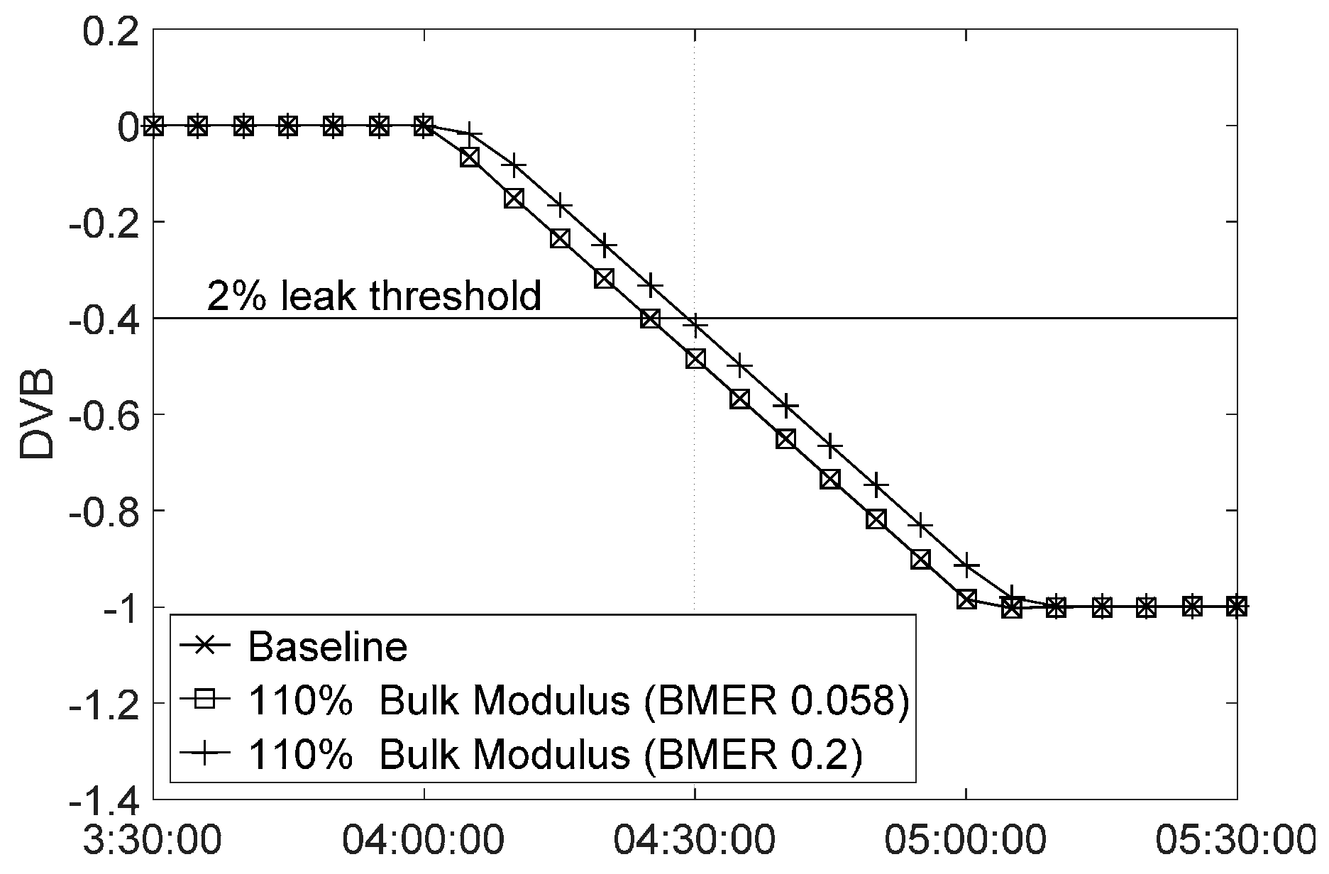
In addition, it was found that the exact amount of required correction must be specified in order for Statefinder to make full correction to the bulk modulus. This can be shown with Figure 6. Two cases were tested, both with +10% bulk modulus error, but the allowable correction (BMER) was set to be exactly the amount needed (0.058) in one case and larger (0.2) in the other case. It can be seen that the DVB curve for the case with the larger BMER deviated from the other case and the baseline. The detection time was delayed for 4.8 min compared to the detection time of 25.5 min for the baseline case. Therefore, if the allowable correction is set too large, Statefinder will make an over-correction to the wave speed, resulting in degraded leak detectability. This is unlike the case with viscosity uncertainty, for which errors can be corrected properly as long as the maximum allowable correction is set greater than the amount of required correction. Therefore, it is clearly more important to have accurate bulk modulus information than accurate measurements of viscosity.
A similar trend was observed with noisy data, as shown in Figure 7. The leak detection was delayed for cases with −10% error in bulk modulus because Statefinder made an incorrect adjustment (i.e., incorrect sign) to the wave speed. The detection time was delayed by 4.9 and 7.1 min from the 33.1 and 61.7 min for the baseline case for the flow decrease and flow increase transients, respectively. The cases with +10% error in bulk modulus were less affected than the −10% error case but not exactly overlapped with the baseline. The detection time was early by 1.0 and 4.6 min for the flow decrease and flow increase transients, respectively. This was because the BMC value was oscillating due to the presence of data noise; thus, exact correction could not be applied.

3.2. Uncertainty in Supervisory Control and Data Acquisition Data

Polling times of 1 s, 5 s, and 10 s were tested and found to have no effect on leak detectability, even during transient conditions. The DVB curves for the cases with 5 s and 10 s polling time overlapped the baseline case (1 s polling time), for both perfect data and noisy data tests.
It was noted that when time skew is present in the measured data, false diagnostic flow can be produced even when there is no leak. In this case, the leak detection system needs to be configured with increased pressure and flow rate repeatability in order to avoid false leak alarms. Statefinder is then allowed to adjust the measured flow rate or pressures by a greater amount. In Figure 8, DVB curves are plotted for cases with time skew set to 10 s in one or two sensors and no time skew in the remainder during transient conditions with perfect data. Only results produced by positive shifts that are shown as negative shifts were shown to have the same effect. It can be seen that the detection time was delayed slightly for all these cases, ranging from 0.5 to 3.3 min compared to the baseline case. The detection time for the corresponding baseline cases was 24.9 and 26.1 min during flow decrease and flow increase transients, respectively. It was noted that the delay in detection time was greatest for cases with time skew in both sensors located at the transient initiation location. For the cases in which the flow rate was decreased at the downstream end, the case with time skew in both the downstream pressure and flow rate sensors located at the downstream end experienced the largest delay of 3.1 min. The flow was increased at the upstream end for the flow increase transient and the case with time skew in the upstream pressure and flow rate sensors had the largest delay of 3.3 min. Note that leak detection times during steady state operations with perfect data were not affected by time skew.
The delay was more pronounced in the cases with noisy data, as shown in Figure 9. Time skew had a larger impact on leak detectability during both steady state and transient operating conditions. Leak detection was delayed by 35 min compared to the baseline case detection time of 33.1 min during a flow decrease transient (Figure 9a). For steady state and flow increase cases (Figure 9b,c), the leak became undetectable compared to detection times of 41.7 and 61.7 min for the corresponding baseline cases. DVB eventually stabilized at −0.22 and −0.08 for the steady state and flow increase cases; both were above the leak detection threshold.

3.3. Low R System vs. High R System

The effect of uncertainties on leak detectability in systems with low and high R values was compared as they have distinctly different hydraulic responses. Computed leak detection times are summarized in Table 5 along with the corresponding viscosity error, bulk modulus error, and time skew for each case. The change in detection times relative to the corresponding baseline case are also tabulated, and negative numbers indicate earlier detection times compared to the baseline case. However, these were associated with excessive diagnostic flow caused by uncorrected errors rather than a leak. Note that setting VER to the same value in the two systems results in a significantly smaller FPDC bound in the low R system, as the portion of the bound that is amplified by VER is proportional to the flow rate. The magnitude of the correction that can be made to the viscosity error in the low R system is much less compared to the high R system. Therefore, VER was set to different values in the low and high R systems to obtain the same FPDC bound in order to make a fair comparison. VER was set to its maximum value of 100% in the system with R = 0.49, which produced an FPDC bound ranging from 0.153 to 0.162 depending on the flow rate after transient. This bound range was equivalent to VER of 2–14% in the system with R = 2.20.
For the perfect data tests in Table 5, there was no clear indication of whether leak detectability was better in high R or low R systems. However, uncertainties had only a minor impact on leak detectability when the “measured” data contained no noise. Thus, it was not essential to determine the fine distinctions observed between the low R and high R systems. For noisy data tests, however, the change in detection time from the baseline case was smaller in the low R system when comparing to the corresponding case in the high R system for 11 of the 15 cases. For the remaining four cases, the two with time skew were undetected in both systems (i.e., DVB never crossed the threshold line); the two cases with positive viscosity error had larger detection time change in the low R system, but again, the changes were very minor (within 1.5 min from the baseline). It can be concluded that in most cases, the impact of uncertainties is less in the low R systems compared to high R systems.

3.4. Random Uncertainty Sources

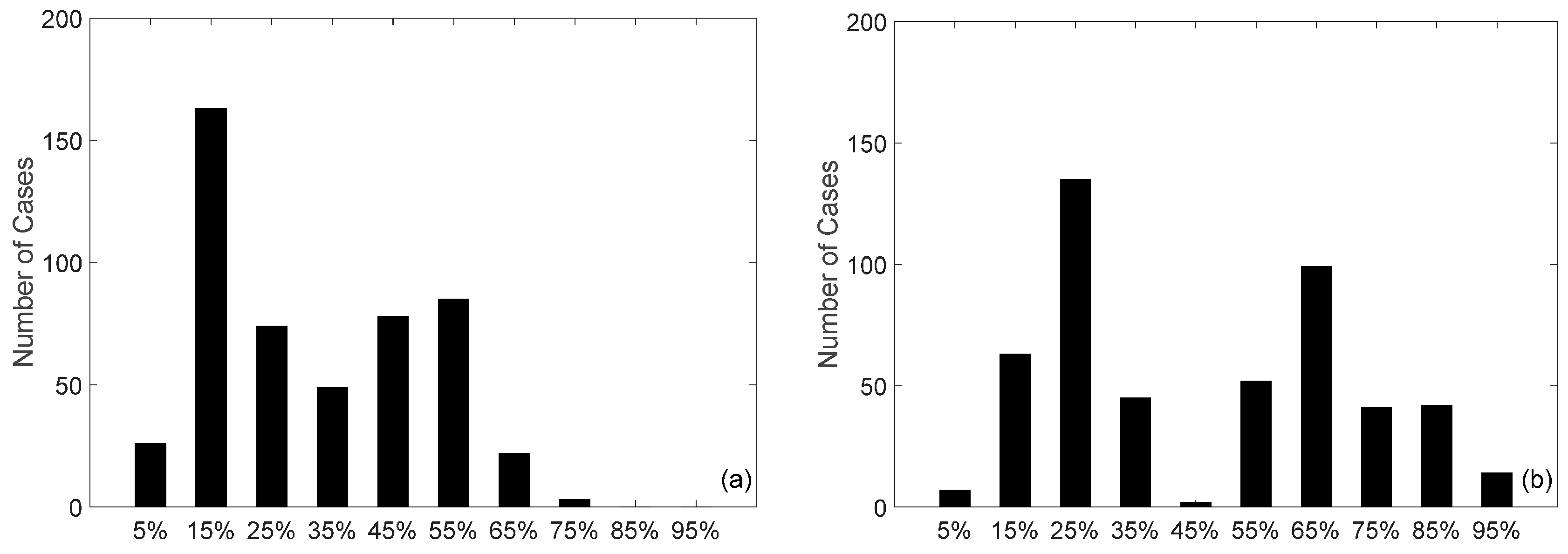
The Monte-Carlo Simulation method was used to generate random values for viscosity, bulk modulus, time skew, polling time, and noise level. The purpose was to observe the probabilistic effect of uncertainties on leak detectability. The hypothesis is that a pipeline system with a low R value is more tolerant of uncertainties compared to a system with a high R value. Here, the baseline was taken as the case without any error in viscosity or bulk modulus, 1 s polling time, no time skew, and with 1% Gaussian noise. For cases experiencing a flow decrease transient, the baseline detection time was 31.1 min for the low R system and 33.1 min for the high R system. In Figure 10a, a histogram is plotted that shows the percentage of delay in the detection time compared to the baseline for the 500 cases, for the low R and high R system, respectively. It can be seen that the presence of random uncertainties caused leak detection to be delayed in all cases. For the high R system, the mean value of the percentage delay was 46.5%, with a standard deviation of 24.8%, and the median was 40.8%. For the low R system, the mean value was 31.8%, with a standard deviation of 17.2%, and the median was 27.3%. This supports the previous finding that leak detection is generally less affected by uncertainties in the low R systems. It is interesting to see that the distribution for the high R system is clearly bimodal with peaks at approximately 25% and 65% in Figure 10b. The data centered around the peaks at 25% and 65% are associated with the cases with 1% and 2% Gaussian noise, respectively. Clearly, the higher the noise level in the “measured” data, the more leak detectability is impacted by uncertainties. This was less clear in the low R system, but a bimodal distribution still exists with peaks at approximately 15% and 55%. There are very few data points at values greater than 60–70%, again supporting the hypothesis that the low R systems tolerate uncertainties better than the high R systems.
Figure 11 summarizes the results for the cases corresponding to a steady state operation. In the low R system, the baseline detection time was 40.2 min, and 285 of the 500 cases were detectable. The mean value of the percentage delay for the detectable cases was 21.3%, with a standard deviation of 13.5% and a median of 19.6% for all detected tests. In the high R system, the baseline detection time was 41.4 min, and only 247 of the 500 cases were detectable. The mean value was 26.7%, with a standard deviation of 14% and median of 22.7%. For the cases experiencing a flow increase transient, all 500 cases became undetectable in either the low R or high R system.

4. Conclusions

This study investigated how various sources of uncertainty affect leak detection with the widely used SPS Statefinder leak detection software [15]. Uncertainties in viscosity, bulk modulus, polling time, time skew, and data noise were investigated. It was found that the SPS Statefinder leak detection system can cope better with errors in viscosity than in the bulk modulus. Leak detectability was unaffected by viscosity errors as long as Statefinder was configured to allow it to fully correct the friction factor. In the case of bulk modulus errors, full correction was only achievable when the bound of the bulk modulus correction coefficient was set equal to the exact amount of required correction and when the pressure wave propagated in a certain pattern. That is, when there is a positive error in the bulk modulus and the transient causes the pressure to increase in the pipeline or there is negative error in the bulk modulus and the transient causes pressure to decrease in the pipeline. A longer polling time alone did not affect leak detectability, but time skew caused a significant degradation of leak detectability during both steady and transient operating conditions when the “measured” data contained Gaussian noise. Therefore, a general ranking of the importance of the uncertainty sources (from high to low) is: (1) time skew, as it always causes degraded leak detectability; (2) bulk modulus error, as it may be incorrectly adjusted in some cases, and the required amount of correction is often not known; (3) viscosity error, as it only has an impact when full correction is not allowed and the data are noisy; and (4) polling time, as it does not affect leak detectability for the cases tested. The probabilistic effect of random uncertainties of all sources caused delayed leak detection in all cases. It was also shown that in general, systems with a lower R factor were less sensitive to uncertainties compared to systems with high R factors. These findings are applicable to a wide category of real-time transient model-based leak detection systems that utilize optimization algorithms to minimize the difference between the modelled and measured pipeline states.

Acknowledgments

This research was funded by a grant from Enbridge Pipelines Inc. and by the Natural Sciences and Engineering Research Council of Canada Collaborative Research Development grant, both of which are gratefully acknowledged.

Author Contributions

Zhe Lu and Yuntong She conceived and designed the study; Zhe Lu performed the study and wrote the draft paper; Yuntong She and Mark Loewen revised and edited the manuscript.

Conflicts of Interest

The authors declare no conflict of interest.

References

  1. National Energy Board. Safety Performance Portal. Available online: https://www.neb-one.gc.ca/sftnvrnmnt/sft/dshbrd/index-eng.html (accessed on 10 October 2016).
  2. Geiger, G. State-of-the-art in leak detection and localization. Oil Gas Eur. Mag. 2006, 32, 193–198. [Google Scholar]
  3. Po, A.; Xing, Y. Internal Free Swimming Pipeline Leakage Detection Technology—Smartball. In Proceedings of the International Conference on Pipelines and Trenchless Technology, Xi’an, China, 16–18 October 2011; American Society of Civil Engineers: Reston, VA, USA, 2011; pp. 996–1005. [Google Scholar]
  4. National Energy Board. Onshore Pipeline Regulations; SOR/99-294; Minister of Justice: Calgary, AB, Canada, 2010.
  5. Province of Alberta. Pipeline Act; Alberta Queen’s Print: Edmonton, AB, Canada, 2014; p. 32.
  6. American Petroleum Institute. Computational Pipeline Monitoring for Liquids; American Petroleum Institute Report 1130; American Petroleum Institute: Washington, DC, USA, 2002. [Google Scholar]
  7. Liou, C.P. Pipeline Leak Detection and Location. In Proceedings of the International Conference on Pipeline Design and Installation, Pipeline Division, American Society of Civil Engineers, Las Vegas, NV, USA, 24–29 September 1990. [Google Scholar]
  8. Al-Khomairi, A. Leak Detection in Long Pipelines Using the Least Squares Method. ASCE J. Hydraul. Res. 2008, 46, 392–401. [Google Scholar] [CrossRef]
  9. He, G.; Liang, Y.; Li, Y.; Wu, M.; Sun, L.; Xie, C.; Li, F. A Method for Simulating the Entire Leaking Process and Calculating the Liquid Leakage Volume of A Damaged Pressurized Pipeline. J. Hazard. Mater. 2017, 332, 19–32. [Google Scholar] [CrossRef] [PubMed]
  10. Al-Zahrani, M. Modeling and Simulation of Water Distribution System: A Case Study. Arab. J. Sci. Eng. 2014, 39, 1621–1636. [Google Scholar] [CrossRef]
  11. Duan, H.F. Uncertainty Analysis of Transient Flow Modeling and Transient-based Leak Detection in Elastic Water Pipeline Systems. Water Resour. Manag. 2015, 29, 5413–5427. [Google Scholar] [CrossRef]
  12. American Petroleum Institute. Pipeline Variable Uncertainties and Their Effects on Leak Detectability; American Petroleum Institute Report 1149; American Petroleum Institute: Washington, DC, USA, 1993. [Google Scholar]
  13. Liou, C.P.; Tian, J. Leak Detection—Transient Flow Simulation Approaches. ASME J. Energy Resour. Technol. 1995, 117, 243–248. [Google Scholar] [CrossRef]
  14. American Petroleum Institute. Pipeline Variable Uncertainties and Their Effects on Leak Detectability; American Petroleum Institute Report 1149; American Petroleum Institute: Washington, DC, USA, 2015. [Google Scholar]
  15. DNV GL Group. Stoner Pipeline Simulator (SPS) 9.9.0 Help and Reference; DNV GL Group: Hong Kong, China, 2012. [Google Scholar]
  16. Wylie, E.B.; Streeter, V.L. Fluid Transient in Systems; Prentice Hall: Englewood Cliffs, NJ, USA, 1993; ISBN 10:0139344233. [Google Scholar]
  17. Canadian Standards Association. Z662-07 Oil and Gas Pipeline Systems: Annex E: Recommended Practice for Liquid Hydrocarbon Pipeline System Leak Detection; Canadian Standards Association: Mississauga, ON, Canada, 2007; pp. 388–392. [Google Scholar]
  18. Vinh, P. Adding Value to CPM Testing; American Petroleum Institute Pipeline Conference and Cybernetics Symposium: Phoenix, AZ, USA, 2012. [Google Scholar]
  19. Modisette, J. State Estimation of Pipeline Models Using the Ensemble Kalman Filter; Pipeline Simulation Interest Group (PSIG): Prague, Czech Republic, 2013; p. 31. [Google Scholar]
  20. Arifin, B.; Li, Z.; Shah, S.L. Pipeline Leak Detection Using Particle Filters. IFAC PapersOnLine 2015, 48, 76–81. [Google Scholar] [CrossRef]
  21. Hung, D.; Mokamati, S. A Novel Approach to Leak Sensitivity Testing of Computational Pipeline Monitoring Systems for Hydrocarbon Liquid Pipelines with Hydraulic Simulators. In Proceedings of the 11th International Pipeline Conference, Calgary, AB, Canada, 26–30 September 2016. [Google Scholar]
  22. Pabon, S. Sensitivity Study of a Computer Model Based Leak Detection System in Liquid Pipelines. Master’s Thesis, University of Alberta, Edmonton, AB, Canada, 2015. [Google Scholar]
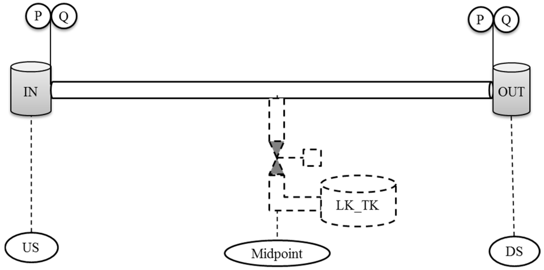
Figure 1. Schematic of the study pipeline with simulated leak.
Energies 10 01226 g001
Figure 2. Effect of uncertainty in R factor on leak detectability in a system with R = 2.20 for a flow decrease transient: (a) perfect data; and (b) noisy data. Arrows in (a) indicate the interception between the threshold line and the DVB curve.
Energies 10 01226 g002
Figure 3. Effect of viscosity error on leak detectability in a system with R = 2.20 with 1% Gaussian noise: (a) flow decrease; and (b) flow increase.
Energies 10 01226 g003
Figure 4. Effect of bulk modulus error on leak detectability in a system with R = 2.20 with perfect data: (a) flow decrease; (b) flow increase.
Energies 10 01226 g004
Figure 5. BMC behaviour for flow decrease transient initiated at: (a) the downstream end; and (b) upstream end with perfect data.
Energies 10 01226 g005
Figure 6. Effect of bulk modulus error on leak detectability with exact and excessive BMER in a system with R = 2.20 with perfect data.
Energies 10 01226 g006
Figure 7. Effect of bulk modulus error on leak detectability in a system with R = 2.20 with 1% Gaussian noise: (a) flow decrease; and (b) flow increase.
Energies 10 01226 g007
Figure 8. Effect of time skew on leak detectability in a system with R = 2.20 with perfect data (sensors contain a 10-s time skew): (a) flow decrease; and (b) flow increase.
Energies 10 01226 g008
Figure 9. Effect of time skew on leak detectability in a system with R = 2.20 with noisy data (sensors contain a 10-s time skew): (a) flow decrease; (b) flow increase; and (c) steady state.
Energies 10 01226 g009
Figure 10. Delayed leak detection time for the 500 cases with random uncertainties under flow decrease conditions in systems where: (a) R = 0.49; and (b) R = 2.20.
Energies 10 01226 g010
Figure 11. Delayed leak detection time for the 500 cases with random uncertainties under steady state conditions in systems where: (a) R = 0.49; and (b) R = 2.20.
Energies 10 01226 g011
Table 1. Level of uncertainties in fluid properties.
VariableVariable ValueEquivalent Error in R
LowerBaseUpperLowerBaseUpper
Viscosity (mPa·s): R = 2.20 system1.314.5711.53−20%0+20%
Viscosity (mPa·s): R = 0.49 system1.694.579.85−20%0+20%
Bulk modulus large (GPa)0.861.453.31+20%0−20%
Bulk modulus realistic (GPa)1.301.451.59+3.5%0−3.0%
Table 2. Tested scenarios of time skew.
Flow ConditionPressure Sensor with Time SkewFlow Meter with Time Skew
Steady State (with leak)USnone
noneDS
USDS
Flow DecreasenoneUS
noneDS
DSNone
DSUS
DSDS
Flow IncreaseUSNone
noneUS
noneDS
USDS
USUS
Table 3. The range of uncertainty for each variable in random error tests.
VariablesRange of UncertaintyTested Values
Viscosity1.31–11.53 mPa·srandom
Bulk modulus1.30–1.59 GParandom
Data noise-1%, 2%
Time skew-5 s, 10 s
Polling time-5 s, 10 s
Table 4. Tuning weights in Statefinder for single error and random error scenarios: Wj (j = 1–7) are weights assigned to measured pressure and flow rate, friction, rate of change of pressure, friction, and bulk modulus, and diagnostic flow, respectively. SCADA: supervisory control and data acquisition.
Tuning WeightsViscosity ErrorBulk Modulus ErrorSCADA ErrorRandom Error
W11111
W21111
W311071071
W410101010
W5500107107500
W610711071
W75555
Table 5. Change in detection time due to uncertainties in systems with low and high R factors.
Data TypeVariableFlow ConditionLevel of UncertaintyBaseline Detection Time (Minutes after Leak Starts)Change in Detection Time (Min)
R = 0.49R = 2.20R = 0.49R = 2.20
Perfect DataBulk ModulusFlow Decrease+10%24.224.90.70.0
−10%1.74.9
Flow Increase+10%24.526.10.50.0
−10%1.47.0
Steady State+10%24.425.50.050.2
−10%−0.05−0.2
Time SkewFlow Decrease10 s24.224.92.5–3.90.6–3.1
Flow Increase10 s24.526.10.8–2.20.5–3.3
Steady State10 s24.425.50.00.0
Noisy DataViscosity 1Flow Decrease−20% f31.133.1−1.8−4.5
+20% f0.20.5
Flow Increase−20% f55.561.7−22.6−34.2
+20% f1.30.1
Steady State−20% f39.841.7−8.7−15.2
+20% f0.5−0.3
Bulk ModulusFlow Decrease+10%31.133.10.1−1.0
−10%0.44.9
Flow Increase+10%55.561.70.0−4.6
−10%1.37.1
Steady State+10%39.841.70.050.2
−10%−0.02−0.3
Time SkewFlow Decrease10 s31.133.128.035.0
Flow Increase10 s55.561.7UndetectedUndetected
Steady State10 s39.841.7UndetectedUndetected
1 Viscosity error was introduced to obtain ±20% error in the friction factor f.