Performance Evaluation of a Hydrogen-Based Clean Energy Hub with Electrolyzers as a Self-Regulating Demand Response Management Mechanism

Abstract

Energy management of hybrid resources has become a critical issue in integrated energy system analysis. In this study, as a self-regulating demand response (DR) management mechanism, deferrable electrolyzers are used as a main controlled resource in a hydrogen-based clean energy hub (CEH), which includes a traditional generation plant (TGP), a low-carbon generation plant (LGP), and wind energy. Based on the hysteresis control model for aggregated electrolyzers, a comfort-constrained optimal energy state regulation (OESR) control strategy is implemented to model the deregulation feature of aggregated electrolyzers. The electrolyzers’ population can be integrated as a controlled efficient power plant (EPP) to provide the virtual spinning reserve for CEH. As a flexible and self-regulating participant, the electrolyzer-based EPP is integrated into the hybrid resource constrained optimization model; this reduces the total cost of CEH and carbon emissions and improves the integration of wind energy. Combined with TGP, LGP, and wind energy, the simulation results show that the deployment of aggregated electrolyzers on both the supply and demand sides of the CEH contributes to significant amounts of low-carbon hydrogen. The simulation also illustrates that the DR control strategy has a positive effect on active power and reserve re-dispatch.

1. Introduction

Improvements in efficient energy utilization and reduction of carbon emissions are among the main factors in the sustainable development of energy systems [1]. To combat global warming, the Paris Agreement was adopted under the United Nations Framework Convention on Climate Change (UNFCCC), with the goal of restricting global temperature increases to below 2 °C above pre-industrial levels [2]. Actions to reduce carbon emissions are key to achieving this goal [3]. However, energy systems are still challenged by managing unsustainable fuel mixtures from various sources, and the integration of renewable energy. High carbon sources, such as coal and oil, are widely used in traditional generation plants (TGPs), thus the overall cost and carbon emissions may increase with growing energy demands [4], subsequently requiring their urgent replacement with clean energy resources. Considering the intermittency and instability of renewable energy [5], low-carbon generation plants (LGPs) using low-carbon energy sources such as nuclear power, and CO₂-sequestered power are required and must be operated on a scheduled power generation plan. The consequent regulation capacity may be insufficient, therefore, the regulation capacity and reserve capacity are primarily supported with TGPs. Furthermore, the lack of reserve capacity may also affect the integration of renewable energy.

Aimed at solving the aforementioned problems, the energy hub concept provides a new way of managing energy in an integrated energy system. Defined as an interface between energy input and energy demand, an energy hub is characterized by multiple energy coupling, effective management through energy conversion and dispatch, and load control on the demand side [6,7]. From the perspective of energy input in an energy hub, hydrogen is regarded as a green energy carrier for clean development due to its low environmental impact and durable nature [8]. Combined with other energy carriers, hydrogen could make the energy systems more flexible and reliable [9]. The produced hydrogen can be fed into the natural gas system using power to gas (P2G) technology, or used in fuel-cell-based transportation and industrial processes. It can be also re-electrified on demand using a fuel cell or directly marketed as a commodity [10]. Accounting for the pathways of energy conversion mentioned previously and environmentally friendly effects, the concept of the energy hub can be extended to the clean energy hub (CEH) [11]. On this basis, the energy management of a hydrogen-based CEH is the primary focus of this study.

Economic and environmental factors require a large yield of hydrogen. Water electrolysis is considered the simplest solution to isolate hydrogen, as it splits water into positively charged hydrogen ions and negatively charged oxygen ions. However, from the perspective of a device level, electrolyzers are widely spatially-distributed in large numbers, which make up a relatively high percentage of energy demand profile. Thus modeling methods and control strategies need to be further exploited.

Combined with load control technologies, utilization of the load aggregation characteristics plays a crucial role in CEH energy management. Considering operational constraints, aggregated small-scale electric loads can be regarded as a dispatchable resource [12]. In this way, an effective integration mechanism for electrolyzer load is an efficient power plant (EPP) as discussed in [13,14]. The electrolyzer-based EPP model can exist as a distributed generator in a hydrogen-based CEH to facilitate resource regulation if implementing a reasonable control strategy; it also provides ancillary services and facilitates the integration of renewable energy.

Previous research [15,16] has shown that in a hydrogen-based energy system with high wind power penetration, a controlled electrolyzer population can be regulated as a load management mechanism for:

(1)

Enhancing resilient economic dispatch, which minimizes the wind curtailment while offsetting wind fluctuations and increasing the system reserve capacity;

(2)

Reducing environmental pressures, by generating hydrogen with a zero/low-carbon footprint.

However, detailed electric-to-hydrogen load dynamics and the deferrable nature of the electrolyzer have not been studied enough to reflect the energy constraints and the characteristics of self-regulation of electrolyzers. Both are necessary to access more realistic operational effects and enhance the regulation reserve capacity.

To obtain a synergistic control on both the system level and device level of an EPP, effective control strategies are necessary. Various control strategies are implemented to account for load types and control targets. In [17], a comfort-constrained demand response (DR) control for distributed heat pump systems was proposed to provide ancillary services, such as the spinning reserve for power systems with higher energy efficiency. In [18], a queuing-controlled strategy with lock-on and off constraint was proposed to control the aggregated thermostatically controlled loads, including water heaters. The queuing-controlled strategy enables thermostatically controlled appliances to provide the auxiliary service for frequency regulation and stable operation. In [19], an energy-constrained state priority list model was established to analyze the charging response of aggregated deferrable electrolyzer units. In this study, an optimal energy state regulation (OESR) control strategy is proposed to aggregate electrolyzer loads, which has the following advantages:

(1)

It is characterized by its ability to accurately respond to the control target.

(2)

It satisfies system-level decision-making while considering user comfort constraints.

(3)

It can be utilized to regulate the variability of renewable energy and filter larger fluctuations [13].

By applying the proposed control strategy, electrolyzer aggregation can be utilized as a self-regulating DR management mechanism. Once the model for an operational-constrained electrolyzer-based EPP is developed, the economic and environment impacts of its operation and optimal dispatch can be evaluated to determine the online resource response (for both supply and demand sides) within the framework of the CEH energy management. In this study, a novel hybrid resource-constrained CEH optimization model is studied to integrate electrolyzer-based EPP, TGP, LGP, and wind power. As a flexible participant, the electrolyzer-based EPP is capable of providing reserve capacity and mitigating the wind curtailment problem due to increased wind energy penetration [20]. This illustrates that the DR control strategy has a positive effect on active power and reserve re-dispatch. In addition, carbon emissions can be reduced due to EPP reserve shifting, where the generation burden is transferred to low-emission units.

This paper is organized as follows. In Section 2, the comfort-constrained DR models to control distributed electrolyzers are presented to describe the electrolyzer-based EPP modeling. The hybrid resource-constrained operation optimization model, and the CEH energy management solution are presented in Section 3. The modeling and simulation results with case studies are discussed in Section 4, and the conclusions, as well as the scope of future work, are summarized in Section 5.

2. Optimal Energy State Regulation for a Control Based Efficient Power Plant with Distributed Electrolyzers

2.1. Hysteresis Control Model of Aggregated Electrolyzers as Deferrable Loads

As typical electricity-to-hydrogen conversion devices [19], electrolyzers are regarded as deferrable loads with the ability to operate under a flexible schedule on the demand side. When implementing an appropriate control strategy, better load management controllability can be obtained. In [21], a hysteresis control model is presented to control the device-level deferrable loads within a user defined comfort zone, providing system ancillary services. In this study, such a control model is employed to increase the controllability of spatially-distributed electrolyzers. The hysteresis control of electrolyzers is shown in Figure 1.

There are two states in the charging process, standby (inactive-state) and charging (active-state). A deadband space δ should be defined according to the needs of end-use measurements, within which electrolyzers maintain their machine-state, i.e., inactive or active. Otherwise, any measurement outside this region results in a change in the energy state (or energy status) of electrolyzers. For example, if the energy trajectory exceeds the upper threshold of the deadband, the machine state of the electrolyzers is transformed from active to inactive, and vice versa. The deadband width is an important parameter for operation quality. By choosing this type of control, a rapid cycling of electrolyzer charging operation can occur with a noisy input, and a definite set point objective can be prevented [21].

For electrolyzers, the control objective is to achieve a desired level of hydrogen energy storage at the end of the operation cycle. This corresponds to a certain amount of charging energy accumulated over a user specified charging horizon. As discussed in [21], denoting the charging trajectory over the charging-horizon as $T_{\mathit{ES}}$, the end-use constraints are given by:

$$\begin{array}{cc}E(T_{\mathit{ES}})={\displaystyle {\int }_0^{T_{\mathit{ES}}}{\eta }^H{P}_{r}n[t]dt\ge E_c};& E[0]=0\end{array}$$

(1)

where $T_{ES}$ is the charging-horizon, ${\eta }^H$ is the one-way energy conversion efficiency, $P_r$ is the rated power of a single electrolyzer, $n[t]$ is the machine state of a single electrolyzer at time $t$, $E_c$ represents the desired level of energy.

Considering the equation above, it is clear that the electrolyzer can charge within the user defined timed bounds, namely:

$${\eta }^H{P}_R>E_c/T_{\mathit{ES}}$$

(2)

By changing the machine-state trajectory, the energy trajectory of electrolyzers can be deferred over the user-set charging horizon without disrupting their functionality for end-users.

As the measurements sample the energy state periodically, by controlling the operational state trajectory of energy conversion, they thereby discretize the system. Hence, mathematically, the hysteresis control logic for a charging process can be written as:

$$n_i[k+1]=\{\begin{array}{l}\begin{array}{cc}1& {\epsilon }_i[k]\le {\epsilon }_{-}\end{array}\\ \begin{array}{cc}0& {\epsilon }_i[k]\ge {\epsilon }_{+}\end{array}\\ \begin{array}{cc}{n}_i[k]& otherwise\end{array}\end{array}$$

(3)

where k is the counter of simulation, $\epsilon$ represents the sampled energy state comparison. ${\epsilon }_{+}$ and ${\epsilon }_{-}$ represent energy state index of lower and upper boundaries:

$$\epsilon [k]=\frac{E[k]-E_{\mathit{ES}}[k]}{E_c}$$

(4)

where $E_{\mathit{ES}}$ is the set point energy level. In this study, ${\epsilon }_{+}$ and ${\epsilon }_{-}$ are assumed to be close to the set point data:

$${\epsilon }_{\pm }=\pm \frac{\delta }{2}$$

(5)

with $\delta$ as the deadband width.

For electrolyzers, the primary objective of the device-level controller is maintaining the charging trajectory determined by Equation (1). The value of $E_{\mathit{ES}}$, therefore, represents a charging schedule that is maintained to ensure the device meets the end-user’s desired energy level by the end of the charging horizon, given by:

$$\begin{array}{cc}{E}_{\mathit{ES}}[k+1]=E_{\mathit{ES}}[k]+\frac{E_c}{T_{\mathit{ES}}}T;& E_{\mathit{ES}}[0]=0\end{array}$$

(6)

where T is the sample period.

2.2. Optimal Energy State Regulation Control Strategy

The OESR control strategy is integrated in this study to achieve an accurate control over the aggregated population of electrolyzers [14]. As shown in Figure 2, there are two groups of electrolyzers in the system, namely the inactive (${\varphi }_0$) and active (${\varphi }_1$) groups with a deadband width $\delta$. If a small regulation $u$ is applied to the virtual set point of the energy state, partial synchronization of energy-constrained electricity-to-hydrogen loads will provide a dynamic response in the power demand. Transitions between the active and inactive machine states will alter the number of groups of electrolyzers, thus varying the total power consumption. By solving the optimal regulation $u^{*}$, the target power consumption to follow a certain objective can be achieved.

Control of the electrolyzer population is achieved by controlling a single electrolyzer. The machine-state $n$ (equaling 1 for active and 0 for inactive) of a single electrolyzer $i$ can be assessed by applying a perturbation $u$ to the end-use function:

$$n_i[k+1]=\{\begin{array}{l}\begin{array}{cc}1& {\epsilon }_i[k]\le {\epsilon }_{-}+u^{}[k]\end{array}\\ \begin{array}{cc}0& {\epsilon }_i[k]\ge {\epsilon }_{+}+u^{}[k]\end{array}\\ \begin{array}{cc}{n}_i[k]& otherwise\end{array}\end{array}$$

(7)

The electrolyzers near the deadband boundaries (also called state transition boundaries) will respond to the regulation signal $u$. It is assumed that the bi-directional communication between electrolyzer appliances and the system central controller is functional. The population dynamics can be described in real-time using direct measurements. Thus power state vectors of the controllable loads can be obtained, which includes information of machine-state, energy state and electrolyzer power consumption. The power state vectors can be used to generate the power density distribution function for both the active and inactive machine states, which describes the amount of power at a given charging state relative to the total installed power existing in the participating population [13]. Since the total power prevailing in the active state defines the aggregated load, the current level can be expressed in terms of the total power in the current responsive population $P_{\mathit{cap}}$ and a capacity-factor Φ, which is given by:

$$P_E(t)=P_{\mathit{cap}}(t)\mathsf{\Phi }(t)$$

(8)

The capacity factor can be calculated in the discrete form as follows [21]:

$$\begin{array}{l}\mathsf{\Phi }[m,k+1]={\displaystyle \sum _{m=0}^{{\epsilon }_{-}}{\varphi }_0[m,k]\Delta \epsilon }+{\displaystyle \sum _{m=0}^{{\epsilon }_{+}}{\varphi }_1[m,k]\Delta \epsilon }\\ {\epsilon }_{+}=m_s+\delta /(2\Delta \epsilon ),\hspace{1em}{\epsilon }_{-}=m_s-\delta /(2\Delta \epsilon )\end{array}$$

(9)

where $m$ is the index for end-use measurement within the deadband space, $m_s$ is the energy state index corresponding to the set point, and $\Delta \epsilon$ is the interval between possible energy state measurements.

Therefore, the aggregated power consumption $P_E$ to produce hydrogen at k + 1 step can be calculated as follows:

$$P_E[k+1]=P_{\mathit{cap}}[k]\left({\displaystyle \sum _{m=0}^{{\epsilon }_{-}}{\varphi }_0[m,k]\Delta \epsilon }+{\displaystyle \sum _{m=0}^{{\epsilon }_{+}}{\varphi }_1[m,k]\Delta \epsilon }\right)$$

(10)

The following problem is to determine a solution $m_s^{*}$ that corresponds to the target $P_E^{*}$, this can be solved directly using the normal Newton-type method or construction of an optimization model [14]:

$$P_E^{*}[k+1]=P_{\mathit{cap}}[k]\mathsf{\Phi }[m_s^{*},k+1]=P_{\mathit{cap}}[k]\left({\displaystyle \sum _{m=0}^{{\epsilon }_{-}^{*}}{\varphi }_0[m,k]\Delta \epsilon }+{\displaystyle \sum _{m=0}^{{\epsilon }_{+}^{*}}{\varphi }_1[m,k]\Delta \epsilon }\right)$$

(11)

where $m_s^{*}$ is the energy state index corresponding to the set point after controlled (the optimal solution). The target $P_E^{*}$ is obtained from the hybrid resource constrained optimization of the CEH.

The optimal set point index $m_s^{*}$ is then converted to a corresponding set point regulation by:

$$u^{*}[k]=\delta \left(\frac{2m_s^{*}[k]}{\Re }-1\right)$$

(12)

where $\Re$ is the discretization resolution.

Preventing access to loads for over half of the deadband during each operating cycle, and guaranteeing that each system displays a somewhat natural duty cycle and passes through the user’s desired set point, the variable $u^{*}$ should observe the following constraint [22]:

$$\left|u^{*}\left[k\right]\right|\le \frac{\delta }{4}$$

(13)

2.3. Comfort-Constraint Based Efficient Power Plant Modeling

The comfort-constraint mainly refers to the expectations of the end-use function to produce hydrogen. Considering other user defined constraints, such as the limitations in the communication and control infrastructure, the state-equation given by Equation (11) is constrained by stipulating the maximum and minimum set point variations. Therefore, if the bandwidth of the regulation signal is expressed as $[u_{min}(m_{s,min}),u_{max}(m_{s,max})]$, as shown in Figure 2, the limits of the aggregated power consumption to produce hydrogen can be calculated as follows:

$$\{\begin{array}{l}{P}_{E,\mathit{max}}[k+1]=P_{\mathit{cap}}[k]\left({\displaystyle \sum _{m=0}^{{\epsilon }_{-,max}}{\varphi }_0[m,k]\Delta \epsilon }+{\displaystyle \sum _{m=0}^{{\epsilon }_{+,max}}{\varphi }_1[m,k]\Delta \epsilon }\right)\\ P_{E,\mathit{min}}[k+1]=P_{\mathit{cap}}[k]\left({\displaystyle \sum _{m=0}^{{\epsilon }_{-,min}}{\varphi }_0[m,k]\Delta \epsilon }+{\displaystyle \sum _{m=0}^{{\epsilon }_{+,min}}{\varphi }_1[m,k]\Delta \epsilon }\right)\\ {\epsilon }_{+,max}=m_{s,max}+\delta /(2\Delta \epsilon ), {\epsilon }_{-,max}=m_{s,max}-\delta /(2\Delta \epsilon )\\ {\epsilon }_{+,min}=m_{s,min}+\delta /(2\Delta \epsilon ), {\epsilon }_{-,min}=m_{s,min}-\delta /(2\Delta \epsilon )\end{array}$$

(14)

The bound power consumption dynamics of an electrolyzer load population can be aggregated and treated as an EPP model under steady-state conditions, allowing a seamless integration with typical operational strategies, as shown in Figure 3. The operators can control the load group without tampering with the end-use functionality of the targeted devices, as the end-use comfort-constraints are explicitly embedded in the model [12].

The electrolyzer-based EPP model provides the spinning reserve for the CEH, but unlike the generation reserve, the responsive load reserve is the actual responsive power consumption, and this reserve $R_E$ reflects the potential regulation capacity of a “negative” EPP model for additional CEH operations. Specifically, there are two options, upward and downward regulation capacity:

$$\{\begin{array}{l}{R}_{E,\mathit{max}}^{\mathit{up}}[k]=P_{E,\mathit{max}}[k]-P_E^{*}[k]\\ R_{E,\mathit{max}}^{\mathit{down}}[k]=P_E^{*}[k]-P_{E,\mathit{min}}[k]\end{array}$$

(15)

In this study, the regulation capacity of the individual EPP at the step $k$ is selected as the regulation reserve and is satisfied by:

$$\begin{array}{l}0\le R_E^{\mathit{up}}[k]\le R_{E,\mathit{max}}^{\mathit{up}}[k]\\ 0\le R_E^{\mathit{down}}[k]\le R_{E,\mathit{max}}^{\mathit{down}}[k]\end{array}$$

(16)

If the load reserve cost per unit is defined lower than the traditional generation, the load reserve should be selected as the priority, which can be cut off from the whole original power reserve requirements $R_{\mathit{CEH}}$ for the CEH:

$${\displaystyle \sum R_g}+{\displaystyle \sum R_E}\ge R_{\mathit{CEH}}$$

(17)

3. Hybrid Resource Constrained Optimization and Energy Management Using Wind Energy and Electrolyzer Integration

At the level of optimal scheduling and energy management of a CEH integrating LGP, TGP, and electrolyzers, several system constraints should be considered depending on the location and control strategy of the electrolyzer applications. It is beyond the scope of this study to examine all these specific deployment configurations (i.e., the physical location of electrolyzers, the capacity of hydrogen storage, and infrastructure requirements and power flow modeling and security checking problem) that can be discussed in a follow-up study.

The configuration of the CEH is shown in Figure 4, where the wind farm, LGP and TGP are mainly on the supply side, while a “demand side electrolyzers (DE) stock” is located at or near the main points of hydrogen demand [22]. An additional load consisting of a “supply side electrolyzers (SE) stock” is placed in the supply side, near the wind farm and LGP, to absorb the wind power that cannot be accommodated by the CEH (otherwise curtailed). Transformer and power electronic converter (PEC) are installed for power conversion, while the electricity-to-hydrogen energy conversion is available via electrolyzers. System reserve is taken into account to withstand the uncertainty in the process of energy supply and utilization, maintaining the operation stability of CEH. The system reserve capacity can be provided by TGP, LGP and electrolyzer-based EPP. The electrolyzer-based EPP can be divided into DE-EPP and SE-EPP, and it is also worth mentioning that the TGP is necessary due to its advantageous ability in regulation and response. On the other hand, from the perspective of decarbonization, it is encouraged to replace this TGP with other low carbon sources like LGP and electrolyzer-based EPP. In addition, the fuel mix for each combination of LGP, wind farm and TGP is also required as input data in order to determine the carbon emissions.

The energy demand in a CEH can be met through a variety of energy conversion and dispatch process in response to the specific targets, indicating the potential of energy management. For example, the customer load can be supplied by TGP, LGP or wind power. In order to address this characteristic of flexible dispatch, the mathematical model of the CEH proposed in Figure 4 can be expressed as:

$$\left[\begin{array}{l}{P}_{\mathrm{C}}\\ P_{\mathrm{DE}}\\ P_{\mathrm{SE}}\\ L_H\end{array}\right]=\left[\begin{array}{ccc}{\lambda }_2^{\mathrm{TGP}}{\eta }^T& {\lambda }_3^{\mathrm{LGP}}{\eta }^T& {\lambda }_2^{\mathrm{Wind}}{\eta }^{\mathit{PEC}}\\ {\lambda }_3^{\mathrm{TGP}}{\eta }^T& {\lambda }_2^{\mathrm{LGP}}{\eta }^T& {\lambda }_1^{\mathrm{Wind}}{\eta }^{\mathit{PEC}}\\ 0& {\lambda }_4^{\mathrm{LGP}}{\eta }^T& {\lambda }_3^{\mathrm{Wind}}{\eta }^{\mathit{PEC}}\\ {\lambda }_3^{\mathrm{TGP}}{\eta }^T{\eta }^H& ({\lambda }_2^{\mathrm{LGP}}+{\lambda }_4^{\mathrm{LGP}}){\eta }^T{\eta }^H& ({\lambda }_1^{\mathrm{Wind}}+{\lambda }_3^{\mathrm{Wind}}){\eta }^{\mathit{PEC}}{\eta }^H\end{array}\right]\left[\begin{array}{l}{P}_{\mathrm{TGP}}\\ P_{\mathrm{LGP}}\\ P_{\mathrm{Wind}}\end{array}\right]$$

(18)

$$\{\begin{array}{l}{\lambda }_1^{\mathrm{TGP}}+{\lambda }_2^{\mathrm{TGP}}+{\lambda }_3^{\mathrm{TGP}}=1\\ {\lambda }_1^{\mathrm{LGP}}+{\lambda }_2^{\mathrm{LGP}}+{\lambda }_3^{\mathrm{LGP}}+{\lambda }_4^{\mathrm{LGP}}=1\\ {\lambda }_1^{\mathrm{Wind}}+{\lambda }_2^{\mathrm{Wind}}+{\lambda }_3^{\mathrm{Wind}}=1\end{array}$$

(19)

where ${\lambda }_1^{\mathrm{TGP}}$, ${\lambda }_2^{\mathrm{TGP}}$ and ${\lambda }_3^{\mathrm{TGP}}$ represent the dispatch factors defining power dispatched to reserve capacity, customer load and DE from TGP, respectively; ${\lambda }_1^{\mathrm{LGP}}$, ${\lambda }_2^{\mathrm{LGP}}$, ${\lambda }_3^{\mathrm{LGP}}$ and ${\lambda }_4^{\mathrm{LGP}}$ represent the dispatch factors defining power dispatched to reserve capacity, DE, customer load and SE from LGP, respectively; ${\lambda }_1^{\mathrm{Wind}}$, ${\lambda }_2^{\mathrm{Wind}}$ and ${\lambda }_3^{\mathrm{Wind}}$ represent the dispatch factors defining power dispatched to DE, customer load and SE from the wind farm. $P_{\mathrm{TGP}}$, $P_{\mathrm{LGP}}$ and $P_{\mathrm{Wind}}$ stand for the power supply by TGP, LGP and the wind farm, respectively. $P_{\mathrm{C}}$, $P_{\mathrm{DE}}$, $P_{\mathrm{SE}}$ and $L_H$ denote the demand of customer load, demand side electrolyzer load, supply side electrolyzer load and hydrogen, respectively.

In this study, it is assumed that all the hydrogen produced by electrolyzers are sold for power generation, thus the energy revenue can be included in the optimization model. Hydrogen fuel quality leads to its issues related transportation and storage. By producing the hydrogen locally through distributed electrolyzers, and utilizing the daily quotas immediately, the problems associated with the transportation and storage costs can be avoided [21].

3.1. Objective Function Definition

In order to minimize the system cost while reduce the carbon emissions of the CEH, the optimization objective of economic dispatch can be modeled by a linear programming problem. Considering that there is a limit of wind directly integrated into CEH, the excess part will be curtailed due to system stability considerations [23]. In this regard, the cost for wind curtailment $J_{\mathit{WCU}}$ is integrated into the optimization model:

$$\begin{array}{l}\min (J_g+J_{R_g}+J_E+J_{R_E}+J_{WCU}-J_H)\\ =\min \left(\begin{array}{l}{\displaystyle \sum _{i=1}^{N_g}{A}_{g,i}}{P}_{g,i}+{\displaystyle \sum _{i=1}^{N_g}{A}_{R_g,i}}{R}_{g,i}+{\displaystyle \sum _{i=1}^{N_E}{A}_{E,i}}{P}_{E,i}+{\displaystyle \sum _{i=1}^{N_E}{A}_{R_E,i}}{R}_{E,i}\\ +A_{WCU}{P}_{WCU}-{\displaystyle \sum _{i=1}^{N_E}{A}_{H,i}}{M}_{H,i}\end{array}\right)\end{array}$$

(20)

For the sake of simplifying the representation of the optimization model where:

• $N_g,N_E$: number of power plants and electrolyzers existing in the CEH;
• $J_g$: total energy cost for generation consisting of fuel consumption, O&M and carbon emissions;
• $J_{R_g}$: total reserve cost for generation;
• $J_E$: the energy consumption cost to produce hydrogen for electrolyzers consisting of O&M and carbon emissions;
• $J_{R_E}$: total reserve cost for EPP provision;
• $J_{WCU}$: total cost for curtailed wind;
• $J_H$: the energy revenue from hydrogen power generation;
• $A_g,A_E$: spot prices to define the TGP, LGP and electrolyzer-based EPP environmental cost characteristics;
• $A_{R_g},A_{R_E}$: constant reserve prices for TGP, LGP and electrolyzer-based EPP;
• $A_H,M_H$: energy price of hydrogen power generation and hydrogen energy produced from the CEH;
• $A_{WCU}$: cost defining wind curtail characteristics;
• $P_{WCU}$: wind power being curtailed;
• $P_g,P_E$: power plants (LGP and TGP) outputs and aggregated power consumption to produce hydrogen;
• $R_g,R_E$: power plants (LGP and TGP) reserve and responsive load reserve.

The emissions cost of each generation resource is calculated based on a carbon tax, which we use its current value of $30 per metric ton of carbon dioxide equivalent (MtCO₂eq) [24] in order to monetize the environmental cost of operating a particular generation resource. The model implements numerical values for the other resource parameters can be found in [14]. Considering fuel, operational, and environmental impacts, and the spot price $A_g$ is modeled by:

$$A_g=(C_f^g+C_{\mathit{om}}^g+C{I}_e\cdot C_{\mathit{ct}}^g)/60$$

(21)

where $g$ stands for the number index of LGP and TGP, $C_f^g$ is the fuel cost, $C_{\mathit{om}}^g$ is the operating & maintenance cost, $C{I}_e$ and $C_{\mathit{ct}}^g$ represent greenhouse gas emission intensities and carbon tax caused by power plants, respectively.

As a regulating and reserve revenue evaluation of electrolyzer-based EPP model, several generation-type parameters are also defined from [25]. The spot price $A_E$ for producing hydrogen process is given by:

$$A_E=\frac{1}{60}\left(\frac{C_{\mathit{om}}^H}{LHV}+\frac{C{I}_H\cdot C_{\mathit{ct}}^e}{LHV}\right)$$

(22)

$$A_H=C_H$$

(23)

where $e$ represents number index of electrolyzer-based EPP, $C{I}_H$ is the greenhouse gas caused by hydrogen production process, $C_{\mathit{om}}^H$ is variable operating & maintenance cost for producing hydrogen, $C_{\mathit{ct}}^e$ is carbon tax caused by electrolyzers, $LHV$ represents lower heating value, $C_H$ is the revenue from producing hydrogen.

3.2. Equality and Inequality Constraints

Equality constraints of CEH energy balance can be obtained by Equations (18) and (19). The flexible energy dispatch is crucial for the hybrid resource constrained optimization. The OESR control strategy and the application of electrolyzer-based EPP exert great impacts on power and reserve re-dispatch, making the aggregation of distributed electrolyzers acts as a dispatchable short term energy balancing resources [17]. The equality constraints of CEH dispatch factors can be illustrated as:

$$\{\begin{array}{l}{P}_{\mathrm{DE}}+P_{\mathrm{SE}}={\displaystyle \sum _{i=1}^{N_E}{P}_{E,i}}\\ P_{\mathrm{DE}}={\lambda }_3^{\mathrm{TGP}}{P}_{\mathrm{TGP}}{\eta }^T+{\lambda }_2^{\mathrm{LGP}}{P}_{\mathrm{LGP}}{\eta }^T+{\lambda }_1^{\mathrm{Wind}}{P}_{\mathrm{Wind}}{\eta }^{\mathit{PEC}}\\ P_{\mathrm{SE}}={\lambda }_4^{\mathrm{LGP}}{P}_{\mathrm{LGP}}{\eta }^T+{\lambda }_3^{\mathrm{Wind}}{P}_{\mathrm{Wind}}{\eta }^{\mathit{PEC}}\end{array}$$

(24)

The output of power plants LGP, TGP and electrolyzer-based EPP should be limited into:

$$P_{g,min}\le P_g+R_g\le P_{g,max}$$

(25)

$$P_{E,min}\le P_E-R_E\le P_{E,max}$$

(26)

where $P_{g,min}$ and $P_{g,max}$ represent power outputs limits of LGP and TGP, $P_{E,min}$ and $P_{E,min}$ represent feasible boundaries of aggregated power consumption of electrolyzers.

Meanwhile, the ramping constraints of controlled units and loads to provide the regulation reserve are summarized as:

$$-r_{g,min}\Delta t\le P_g[k+1]-P_g[k]\le r_{g,max}\Delta t$$

(27)

$$-r_{E,min}\Delta t\le P_E[k+1]-P_E[k]\le r_{E,max}\Delta t$$

(28)

where $r_g$ and $r_E$ represent the ramping constraints of power plants and controlled electrolyzers.

A set of constraints for supplying reserve are also defined for all the units and loads:

$${\displaystyle \sum _{i=1}^{N_g}{R}_{g,i}}+{\displaystyle \sum _{i=1}^{N_E}{R}_{E,i}}\ge R_{\mathit{CEH}}$$

(29)

All the components of supply and demand side should be non-negative:

$$\begin{array}{ll}{P}_i\ge 0;& i\in (\mathrm{TGP},\mathrm{LGP},\mathrm{Wind});\\ P_j\ge 0;& j\in (\mathrm{C},\mathrm{DE},\mathrm{SE})\end{array}$$

(30)

3.3. The Energy Management Solution for Clean Energy Hub

In this study, the CEH functions as an interface between the energy producer (TGP, LGP, and wind energy) and the consumer (customer loads and electrolyzers). The diversities of the fuel mixture on the supply side highlight the flexibility and optimization potential of a CEH. Given that the integration of renewable energy and reduction of carbon emissions are stressed as the optimization objective, energy replacement in the CEH is encouraged for the sake of the economy and environmental benefits. However, the TGP is necessary because it provides the system reserve that maintains the operational stability. In this regard, it is actually a trade-off between the economy, environment, and system stability. Thus, it is vital to coordinate with various low carbon resources. Among these, the load management plays a significant role, and an accurate and reasonable DR control strategy is the key issue.

The energy management solution for the CEH consists of three primary parts: the OESR control strategy stage, the EPP modeling stage and the optimization stage, as illustrated in Figure 5.

After the CEH structure and the operation parameters are set in the initialization process, the CEH energy management starts from the OESR control strategy stage. With the application of the hysteresis control, the deferrable characteristic of electrolyzers is enhanced and thus the controllability of the aggregated electrolyzers can be improved. Based on this, the OESR control strategy is implemented to achieve the accurate and effective management of aggregated populations of controllable loads in response to the optimal target, which is updated from the hybrid resource constrained optimization process.

In the next stage, by analyzing the bound power consumption dynamics of aggregated electrolyzers, the comfort-constraint based EPP model is established. The EPP comfortable boundaries also elucidate the potential regulation ability in providing the CEH spinning reserve and reducing the TGP output power.

As a flexible and self-regulating participant, the electrolyzer-based EPP is then integrated into the optimization stage, which illustrates that the DR control strategy has a positive effect on active power and reserve re-dispatch. Therefore, the optimal target for the controllable loads in the next time interval can be obtained.

4. Case Studies

The case study part assumes a CEH attempting to pursue a low carbon fuel mix along with the verification of the proposed control strategy of aggregated electrolyzers. The structure of the CEH is illustrated in Figure 4. The conventional generation is defined to consist of both a LGP and a TGP. The LGP, wind farms, as well as the EPP represent the low-carbon resources (the clean energy), while the TGP represents a carbon intensive resource.

Three kinds of loads are considered in the CEH, consumer residential load, DE on the demand side and SE on the supply side. In all cases, customer loads are normal end-use loads, such as air conditioners, lights, and plug loads. The power rating of the electrolyzers is uniformly distributed in a range of 5–20 kW, which is commissioned to produce 0.031 kg/kWh of hydrogen (based on the LHV = 33.3 kWh/kg for hydrogen) over the production period of one day. The efficiency of the production process is sensitive to the voltage applied across the electrolytic cells, where it is assumed that in each case the rated power for an operating unit corresponds to the maximum efficiency associated with the number of electrolytic cells encompassed. A summary of the parameters implemented in the electrolyzer example is provided in

Table A1. Parameters for the device-level simulation of supply and demand side electrolyzers.

Parameter	Description	Value
Pr	Rated power of electrolyzer	5–20 kW
ηT	conversion efficiency of transformer	1
ηPEC	conversion efficiency of PEC	1
ηH	Electrolyzer energy conversion efficiency	0.75
EC	Desired amount of hydrogen (energy content)	0.031 kg/kWh
Ts	Desired time to accumulate total energy	24 h
δ	Hysteresis control deadband width	0.0375

of Appendix A. No other energy storage technologies or load management mechanisms have been considered in the study presented here.

It is assumed that all power plants and controlled electrolyzer loads act to provide regulation service requirements caused by the intermittency of wind power. Electrolyzer operations and emission punishments are considered in this model. All corresponding economic and environmental parameters for units and loads are defined as constant values shown in

Table A2. Parameters used for units and loads.

Gen/Load	Resources Type	AE × 10−3 ($/kW∙min)	AH × 10−3 ($/kW∙min)	CIe (kgCO2/MWh)	CIH (kgCO2/kgH2)	${\mathit{C}}_{\mathit{f}}^{\mathit{g}}$ ($/MWh)	${\mathit{C}}_{\mathit{o}\mathit{m}}^{\mathit{g}}$ ($/MWh)	${\mathit{C}}_{\mathit{o}\mathit{m}}^{\mathit{H}}$ ($/kg H2)	Cct ($/kgCO2)
1	TGP	0.2400	-	0.980	-	13.7	0.70	-	0.03
2	LGP	0.1150	-	0.012	-	6.20	0.07	-	0.03
3	Wind	0.0028	-	0.015	-	0.00	0.17	-	0.03
4	Zero-carbon DE/SE	-	0.0751	-	0	-	-	0.15	0.03

of Appendix A [21]. The optimization model is run over a 24-h time-period at a frequency of 1 min (1440 decision making intervals for regulation time-scales), but the methodology is applicable to any appropriate time based simulation. The main outputs are daily energy balances, load profiles and carbon intensities for electricity. The results are analyzed in terms of the time-varying generation outputs, and two specific scenarios are studied, namely with and without access to a DR control for the electrolyzer loads. The simulation was run on an Intel Core i5-2540M, 2.60 GHz processor with 8 GB of RAM.

To explore the impacts of different parameters on the results, four cases were studied.

Table 1. Brief description of each case study.

Case Number	Description	Controlled Proportion (%)
		DE	SE
Case-1	Controlled electrolyzers are deployed on both the supply side and demand side with fixed wind penetration of 30%.	30	50
Case-2	Scenario A: Controlled electrolyzers are located only on the demand side with fixed wind penetration of 30%.	--	0
	Scenario B: Controlled electrolyzers are located only on the supply side with fixed wind penetration of 30%.	0	--
	Scenario C: Controlled electrolyzers are deployed both on the supply side and demand sides with fixed wind penetration of 30%.	--	--
Case-3	Controlled electrolyzers are deployed on the demand side with different wind penetration.	80	0
Case-4	Scenario A: Controlled electrolyzers are located only on the demand side with different δ and fixed wind penetration of 30%.	50	0
	Scenario B: Controlled electrolyzers are located only on the demand side with different $u_{\max }$ and fixed wind penetration of 30%.	50	0

provides brief descriptions of the four cases.

4.1. Case-1: Aggregated Charging Performance of Efficient Power Plant Based on Optimal Energy State Regulation Control Strategy

Wind penetration ${\mathsf{\Phi }}_{\mathrm{Wind}}$ is defined as the ratio of the installed capacity of the wind farm to the maximum system demand (MSD) $P_{\mathit{MSD}}$ [21]. According to [23], there is a 30% penetration limit on the wind power output directed to the grid, as described in the following equation:

$$P_{\mathrm{Wind}}=P_{\mathrm{Wind}\_\mathrm{C}}+P_{\mathrm{Wind}\_\mathrm{DE}}\le 0.3(P_{\mathrm{C}}+P_{\mathrm{DE}})$$

(31)

This implies that the wind will be curtailed whenever the wind energy exceeds 30% of the total system demand (including customer demand and electrolyzers located on the demand side) [21]. For this case, the wind penetration ${\mathsf{\Phi }}_{\mathrm{Wind}}$ is considered as 30%. The 400 DE loads $P_{\mathrm{DE}}$ and 400 SE loads $P_{\mathrm{SE}}$ are located on the demand and supply side, of which 30% of DE loads and 50% of SE loads are controlled. The uncontrolled power consumption for all loads and the wind profile used in the simulation are shown in Figure 6. In this case, the wind power is fully integrated to supply the loads, and the controlled electrolyzers primarily impact the CEH energy dispatch.

Table 2. Numerical values implemented to parameterize the generation and efficient power plant (EPP) model.

Gen/Load	Type	Pmax (MW)	Pmin (MW)	${\mathit{r}}_{\mathit{m}\mathit{a}\mathit{x}}^{\mathit{A}\mathit{G}\mathit{C}}$ (MW)	${\mathit{A}}_{{\mathit{R}}_{\mathit{g}}}$, ${\mathit{A}}_{{\mathit{R}}_{\mathit{E}}}$ ($/kW∙min)	RCEH (MW)
1	TGP	10	2	3	0.165 × 10−3	Equation (33)
2	LGP	4	1	1	0.155 × 10−3
3	DE	Auto	Auto	0.5	0.100 × 10−3
4	SE	Auto	Auto	0.5	0.100 × 10−3

“Auto” indicates that the boundaries for the DE and SE power consumptions are calculated using Equation (14) and are updated each minute.

summarizes the numerical values implemented to parameterize the generation and EPP model in the operation process. In this case, the total reserve is defined as:

$$R_{\mathrm{TGP}}+R_{\mathrm{LGP}}+R_{\mathrm{DE}}+R_{\mathrm{SE}}\ge 0.1R_{\mathit{CEH}}$$

(32)

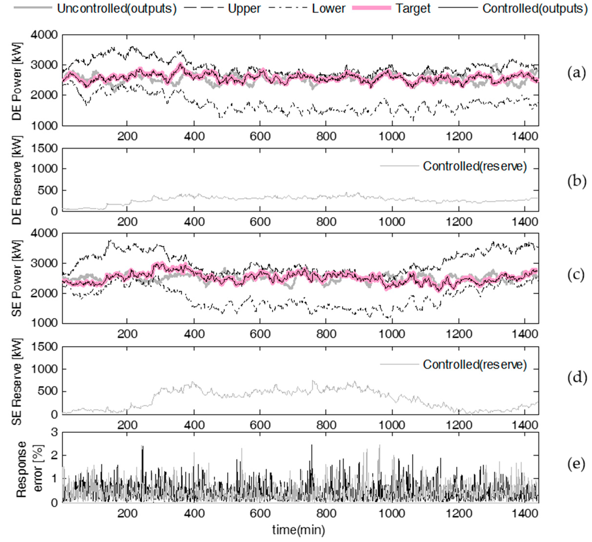
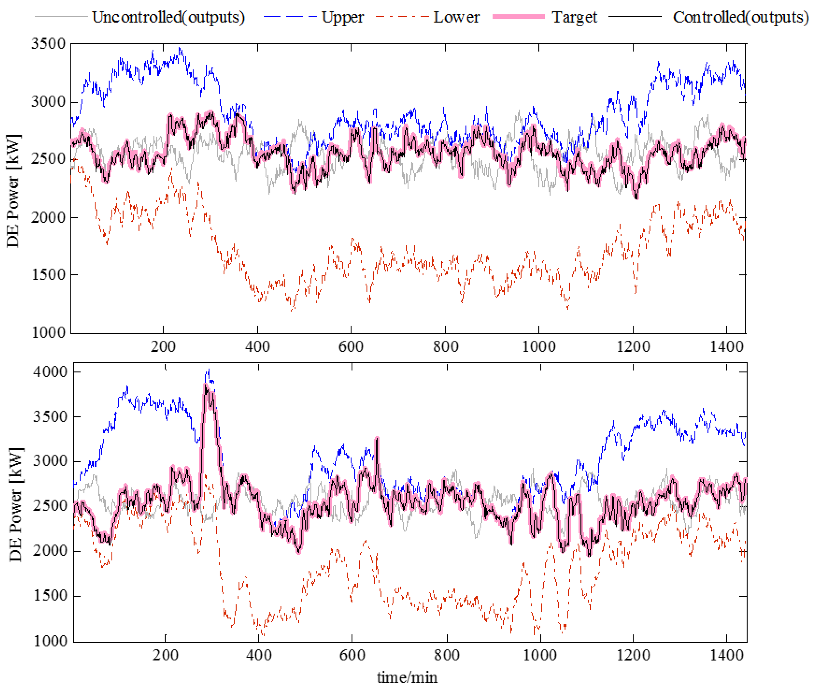
In the simulation results from Case-1, without considering the EPP reserve, the DE and SE loads are operated to maintain a certain region to provide a virtual reserve, as shown in Figure 7b,d. The results show that the actual response of the controlled loads is well aligned with the target, which is obtained from the optimization model in Section 3. Meanwhile, the effective control strategy ensures that maintaining this response generates an error less than 3%, which is expressed as:

$$E_r=\left|(P_E^{*}-P_E)/P_E^{*}\right|\times 100\%$$

(33)

As shown in Figure 7a–c, more hydrogen is expected to be generated to integrate more wind energy, especially when the customer load profile is at its relative valley and wind energy is at its relative peak (Figure 6) during t = 800–1000 min. In addition, the EPP reserve is limited by the feasible operating boundaries of the electrolyzers because the controlled power trajectory has to follow the limits without any variable margin to support this service.

As shown in the Figure 8, the TGP provides more regulation reserve than the LGP due to its flexible regulatory capacity in the uncontrolled scenario. In the controlled scenario, the reserves from the TGP and LGP decrease further due to the integration of the EPP reserve provided by DE and SE. Meanwhile, as seen in Figure 9, the total system cost also decreases by 10.2%, from approximately $705.6 (the uncontrolled case) to $633.6 (the controlled case) per day because the cheaper reserve service is preferred.

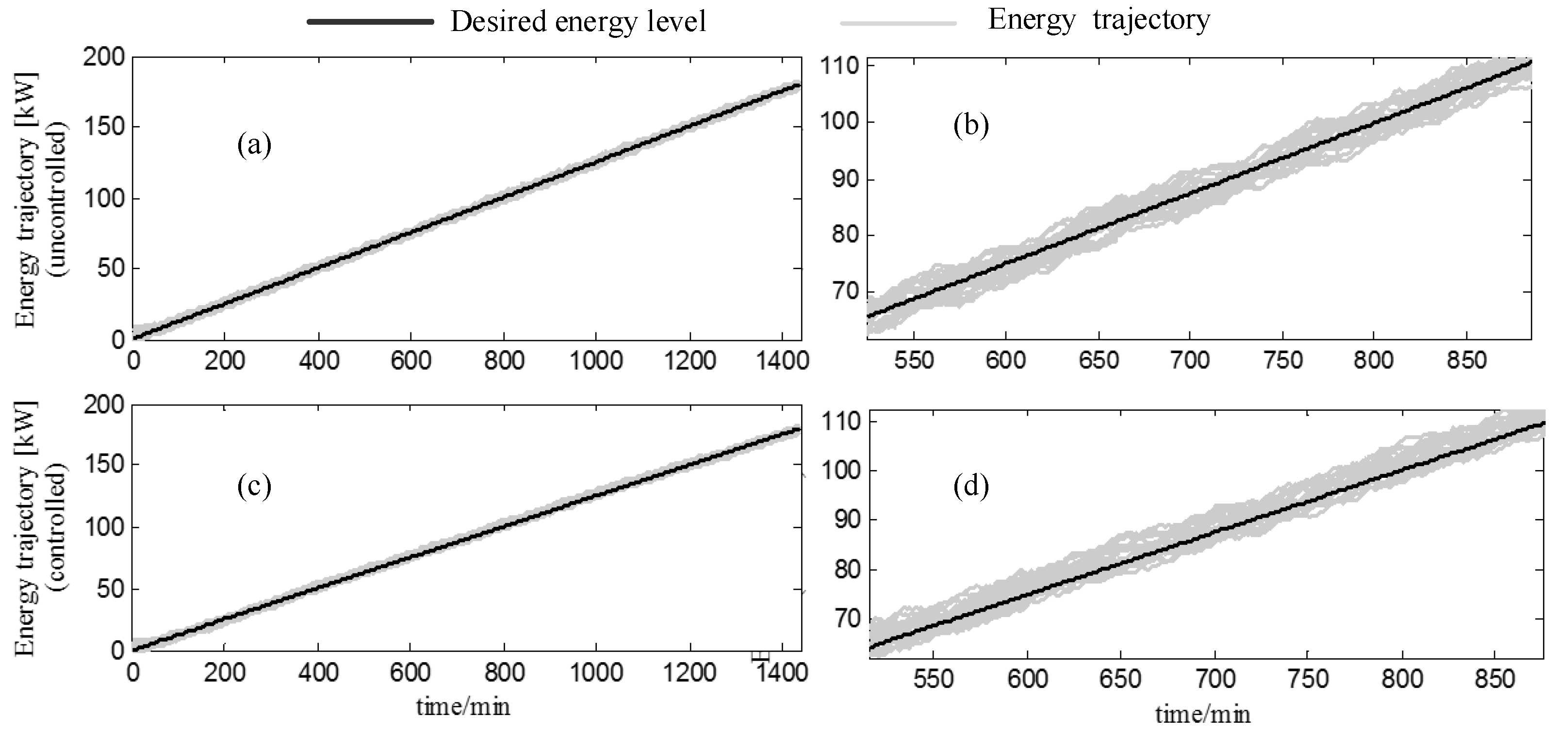
The charging trajectory and relative energy state of the DE are shown in Figure 10 and Figure 11. All the charging energy trajectories of the uncontrolled and controlled scenarios are determined using Equation (1). In the uncontrolled case shown in Figure 10a,b, all energy trajectories are determined with hysteresis control, and in the controlled case, they are modified due to the OESR control strategy, as shown in Figure 10c,d. The trajectories in Figure 10d ascend due to the optimal regulation signal $u$, especially in comparison to energy trajectories in a magnified time range [600, 800].

Similarly, as shown in Figure 11, the energy state for an individual electrolyzer also indicates the control result of the OESR strategy. In particular, there are obvious changes in $n[t]$ that occur in a time range where there are obvious variations in the load following signal $P_E^{*}$. Due to the optimal regulation $u$, the energy state of an individual electrolyzer is operated within the boundary constraints to respond to the optimal target.

4.2. Case-2: Impacts of Increasing the Response Capacity of the Controlled Load

In this case, the proportion of controlled load varies from 0% to 100% of the total DE or SE. The level of wind penetration is 30% and there is no wind curtailment. The electrolyzer parameters are the same as those for Case-1. Three scenarios are simulated. In scenario A, only the DE controlled case was modeled, while in scenario B, only the SE controlled case was modeled. In scenario C, the model coordinated the control of the DE and SE.

The changes of the controlled load response capacity have a significant effect on reserve dispatch and generation plants output power. In general, with the increase of the controlled load proportion, the potential regulation ability of comfort-constraint based EPP is enhanced, and from the perspective of economy and environmental benefits, the task of providing the spinning reserve is gradually undertaken by the EPP. As a self-regulating participant capable of providing the flexible reserve, the integration of EPP also results in the consequent diversities in TGP/LGP output power.

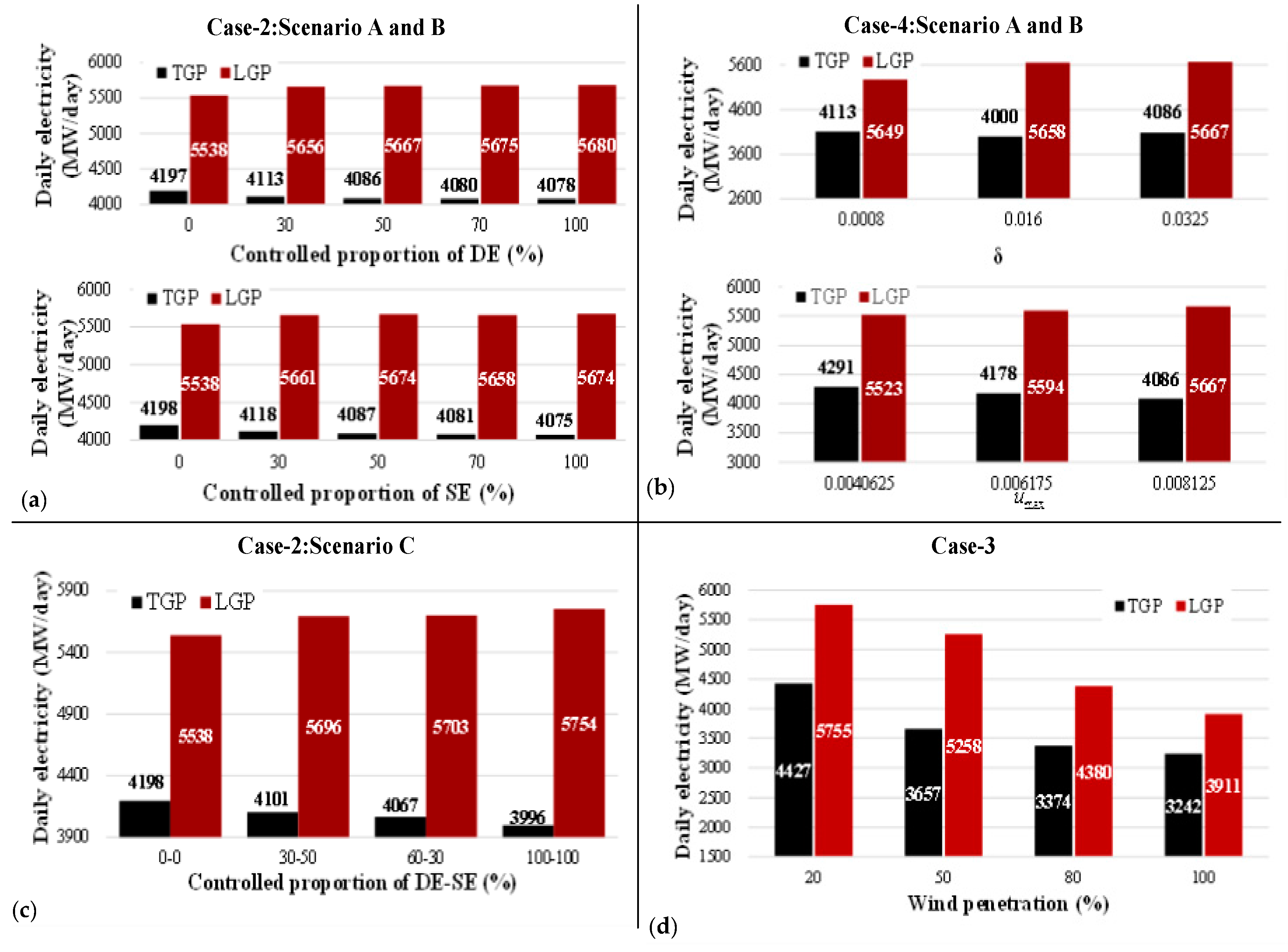
Taking scenario A as the example, the increased proportion of controlled DE causes the significant decrease of TGP and LGP reserve. In contrast, due to the lower cost provided, the DE-EPP virtual reserve rises rapidly, reaching 1129 MW when the controlled proportion of the DE reaches 100%, as seen in Figure 12a.

The diversities of TGP/LGP output power can be illustrated from Figure 13, where the daily electricity from TGP is reduced by 119 MW per day, and that from the LGP increases by 142 MW due to less carbon emissions produced. The output from the TGP has a lower limit to maintain a safe CEH operation.

The aggregated controlled electrolyzers also have the potential to integrate more wind energy, which is even more important when accounting for wind curtailment. As shown in Figure 14a, over 40% of wind electricity is transferred to the DE in the controlled cases. Compared to the controlled proportion 50% and 100%, the wind energy transferred to the DE decreases. There are two possible explanations for this. First, as depicted in Figure 15, a better performance in tracking the target and less power consumption can be achieved as the DE controlled proportion increases. The enhanced potential regulation ability of EPP leads to the decrease of average target power per minute from 2580 kW to 2570 kW, as well as the average upper and lower boundary difference from 1183 kW to 1173 kW, satisfying the comfort constraint of end-use customers. This produces differences in wind power dispatch factor, where ${\lambda }_1^{\mathrm{Wind}}$ (indicating wind power dispatched to DE) decreases from 0.25 to 0.24. Second, although a greater yield of hydrogen is encouraged, the upper limit of hydrogen production is reached before the controlled proportion of the DE reaches 100%. In this regard, more wind energy is dispatched to the customer load and the SE to maintain the energy balance. Considering that SE is not controlled in this scenario, the wind integration with the SE is limited and the customer load consumes more wind energy.

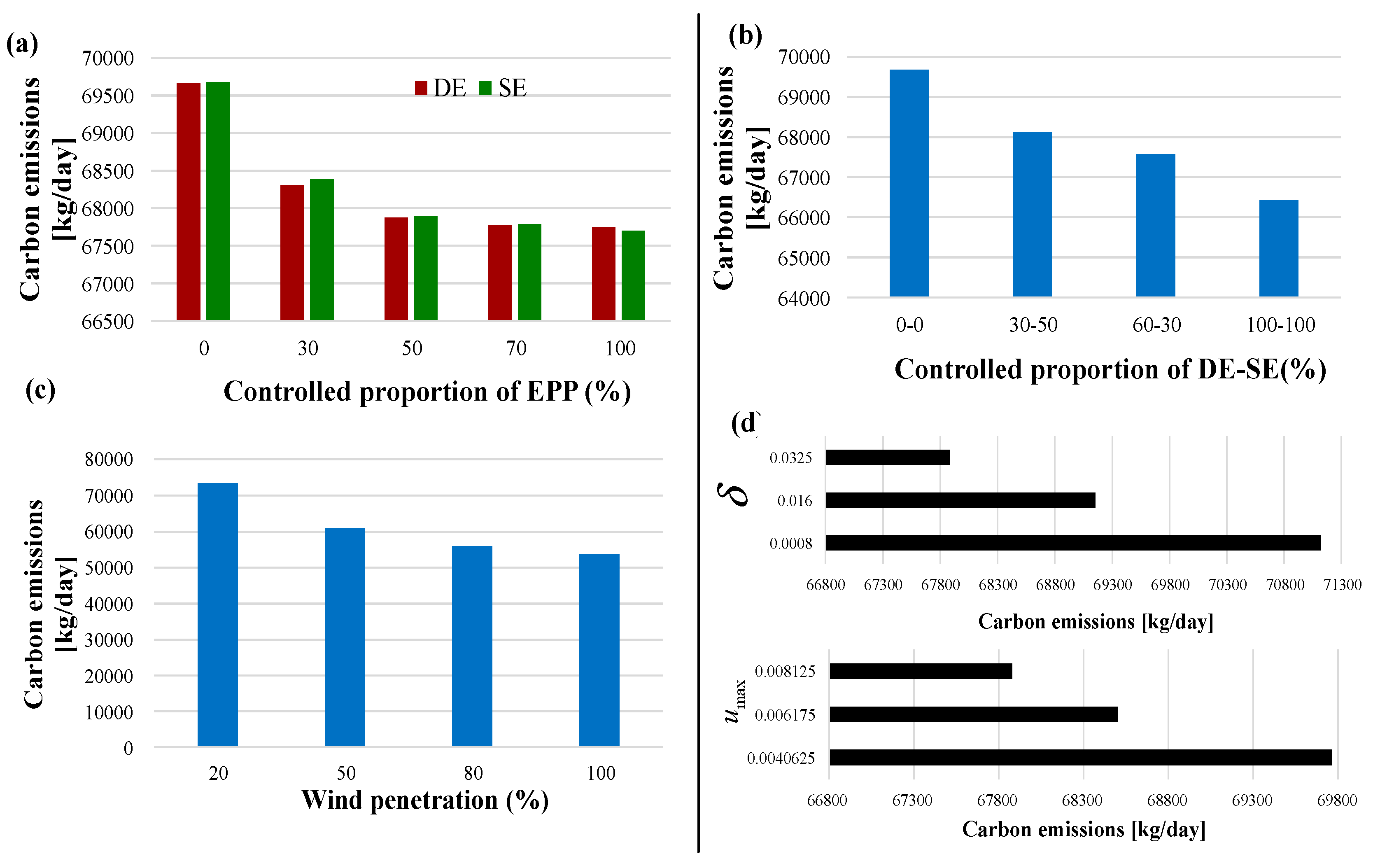
Similar effects can be achieved in scenario B with respect to reserve dispatch and generation plants output power. With the controlled proportion of SE increased, more wind energy can be absorbed by SE to some extent, resulting in the variation of wind dispatch factors. In addition, compared to the uncontrolled case, carbon emissions are reduced by 1913 kg and 1980 kg per day in scenario A and scenario B as illustrated in Figure 16, respectively, showing the environmental benefits of employing the proposed control strategy.

In scenario C, as rendered in Figure 12b, with more DE and SE controlled, the TGP reserve decreases further, to approximately 1182 WM per day; the explanation is clear considering the reserve in the last two scenarios. Taking the controlled situation with a 100% DE and 100% SE participating in the aggregated DR for example, the daily electricity from the TGP is reduced by 202 MW per day while that of the LGP increases by 215 MW. Meanwhile, there is a change in wind power dispatch compared to that in the uncontrolled case (see Figure 14c). There is also a 3300 kg per day decrease in carbon emissions, indicating the changes in the control proportion have a significant impact on reducing the carbon emissions (see Figure 16b). These carbon emissions impacts are a result of (1) the increase of control proportion of DE and SE, which decrease the electricity from the TGP, and (2) much of the reserve is provided by the electrolyzer-based EPP, thus reducing the TGP output.

4.3. Case-3: Impacts from Increasing Wind Penetration

In this case, the wind penetration ${\mathsf{\Phi }}_{\mathrm{Wind}}$ ranges from 20% to 100%. Under some conditions when ${\mathsf{\Phi }}_{\mathrm{Wind}}$ is over the 30% limit, $J_{\mathit{WCU}}$ in Equation (20), which accounts for the wind power curtailment, is adopted. The controlled electrolyzers are located on the demand side with a controlled proportion of 80%. The related parameters, as well as conventional power plants constraints are the same as those in Case-1.

As the wind penetration level increases, the TGP reserve decreases by 756 WM per day while the LGP reserve increases by 369 WM when ${\mathsf{\Phi }}_{\mathrm{Wind}}$ ranges from 20% to 100%, as illustrated in Figure 12c. Due to the fixed response scale of the DE, the virtual reserve is limited. With increasing penetration of wind energy, the LGP reserve increases to reduce the wind curtailment. Similarly, the TGP and LGP output power decrease due to wind integration. Specifically, the TGP output power is reduced by 1185 MW per day while that from the LGP is reduced by 1844 MW when ${\mathsf{\Phi }}_{\mathrm{Wind}}$ reaches 100% (see Figure 13d).

As shown in Figure 14d, with an increase in wind penetration, the amount of wind power transferred to the DE rises in both the controlled (C) and uncontrolled (U) scenarios due to the curtailed wind punishment. The consumption of the DE is inherent and fixed in the uncontrolled scenario; in contrast, with the employment of the OESR control strategy, the enhanced potential regulation ability of DE-EPP facilitates the mitigation of wind fluctuation.

However, due to the upper and lower boundary limitation of DE-EPP in the controlled scenario, there is still some wind that cannot be absorbed, especially when the wind penetration level exceeds 50%, as detailed in

Table 3. Utilization ratio of wind power with different wind penetration values.

Controllable Case	Wind Penetration (%)	20	50	80	100
Uncontrolled	Curtailed ratio (%)	0	0.14	5.75	13.8
	Curtailed power (MW)	0	3	198	593
	Cost for wind curtailment ($)	0	8.4	554.4	1660.4
Controlled	Curtailed ratio (%)	0	0	3.34	8.53
	Curtailed power (MW)	0	0	114.8	367.2
	Cost for wind curtailment ($)	0	0	462.9	1480.5

. Taking the 100% wind penetration controlled case as an example, compared to the uncontrolled case, the curtailed ratio is reduced by 5.27% and $179.9 wind curtailment cost per day can be avoided. The enhancement of DE controllability makes ($P_{\mathrm{C}}+P_{\mathrm{DE}}$) in Equation (31) increase, thus the limit of $P_{\mathrm{Wind}}$ integration is extended.

As shown in Figure 16c, the increase in wind penetration results in fewer carbon emissions from the TGP and LGP. When ${\mathsf{\Phi }}_{\mathrm{Wind}}$ increases from 20% to 100%, the decrease in carbon emissions is approximately 19.7 t per day. The results show that the implementation of DE promotes the wind energy integration, and the application of the proposed control strategy is conducive to reducing carbon emissions.

4.4. Case-4: Impacts of Demand Response Parameter Changes

Apart from the control state of electrolyzers and wind integration factor, the selection of appropriate parameters is also crucial for the effect of the control strategy. In order to obtain the appropriate parameters, two scenarios are studied in this case, showing the impacts of parameter changes on the DR control strategy.

In scenario A, the value of the deadband $\delta$ is assumed to be varied. Three typical values are set to explore the effect, $\delta /4$, $\delta /2$ and $\delta$ (the typical value of $\delta$ is 0.0325). In scenario B, the value of $u_{max}$ is changed. Three typical values are set, $0.5\ast u_{max}$, $0.75\ast u_{max}$, $u_{max}$ (the typical $u_{max}$ is 0.25). The description of the deadband and $u$ are provided in Section 2. For this case, only 50% of the DE is controlled. The level of wind penetration is the same as in Case-1.

As seen in the subplot (d) of Figure 12, Figure 13 and Figure 16, the TGP reserve decreases by approximately 103 MW per day comparing the value of the deadband $\delta /4$ and $\delta$; concurrently, the power output from the TGP decreases and that from the LGP increases. In addition, the performance towards reducing carbon emissions is better achieved when the value $\delta$ is selected. The explanation for these changes is that as $\delta$ increases, the responsive range becomes wider, thus providing a larger reserve capacity. The results also indicate that a reasonable deadband is significant to control effects, the energy operators should define $\delta$ according to the actual target and end user requested comfort.

In scenario B, as shown in Figure 12d, with an increasing $u_{max}$, the reserves of TGP and LGP total decrease and the DE reserve increases. Moreover, as shown in Figure 16d, the carbon emissions also decrease by about 1883 kg per day. As the value of $u_{max}$ gets larger, the controllable boundary is extended. However, the reserve capacity supplied by the TGP and LGP decreases due to the replacement with the DE virtual reserve capacity. The result demonstrates that the value of $u_{max}$ is crucial for determining an OESR $u^{*}$ in the control strategy, and thus it can significantly influence the results. To achieve better results, the definition of $u_{max}$ should be a little more than $\delta /4$, according to Equation (13).

5. Conclusions

This study discusses how DR plays an important role in the energy management of a hydrogen-based CEH, which includes the TGP, the LGP, and wind energy as sources. The comfort-constrained OESR control strategy is implemented to model the deregulation feature of aggregated electrolyzers, as well as explore the potential for optimal target tracking. On this basis, the electrolyzer-based EPP model is established as a dispatchable resources, providing the regulation service to offset the variability of wind power in the self-regulating CEH. The electrolyzer-based EPP can then be integrated into the hybrid resource constrained optimization process, thus the resilient economic dispatch can be obtained, and environmental pressures can be reduced by EPP reserve shifting generation burden to low-emission units. The results also indicate that as a self-regulating DR management mechanism, the aggregation of electrolyzers can provide an effective technical path to support the integration of wind energy. Future work based on this study may include the two following aspects: (1) the coordination of various controllable loads (such as thermostatically controlled loads and plug-in electric vehicles) in the CEH energy management; and (2) the collaborative control of the supply side resources (e.g., synergies of electricity network, natural gas network and hydrogen network) and demand side resources.