A Full Frequency-Dependent Cable Model for the Calculation of Fast Transients

Abstract

The calculation of frequency-dependent cable parameters is essential for simulations of transient phenomena in electrical power systems. The simulation of transients is more complicated than the calculation of currents and voltages in the nominal frequency range. The model has to represent the frequency dependency and the wave propagation behavior of cable lines. The introduced model combines an improved subconductor method for the determination of the frequency-dependent parameters and a PI section wave propagation model. The subconductor method considers the skin and proximity effect in all conductors for frequency ranges up to few megahertz. The subconductor method method yields accurate results. The wave propagation part of the cable model is based on a cascaded PI section model. A modal transformation technique has been used for the calculation in the time domain. The frequency-dependent elements of the related modal transformation matrices have been fitted with rational functions. The frequency dependence of cable parameters has been reproduced using a vector fitting algorithm and has been implemented into an resistor-inductor-capacitor network (RLC network) for each PI section. The proposed full model has been validated with measured data.

1. Introduction

The safe and reliable operation of cable systems requires the analysis of transient behavior of such systems. Single core cables with a core and a shield are utilized prospectively. The first models for the calculations of wave propagation and their transient behavior were developed in the 1970s. The structure of the line models is divided into two main components, a module for calculation of frequency-dependent parameters and the wave-propagation model.

For calculation of the line parameters, Ametani’s algorithm [1] (cable constants) uses the principal assumptions of Wedepohl [2]. Ametani’s algorithm uses a bundle of equations to determine the coupled cable impedances. The frequency-dependent earth return impedance is considered with an fictive earth conductor given by Carson [3] and Pollaczek [4]. The skin effect within the cable core is implemented using Schelkunoff’s equations [5]. The proximity effect between the conductors and the skin effect in the shield are neglected. Morched et al. [6] also use principal assumptions similar to the ideas of Wedepohl [2] and Ametani [1].

The wave propagation models can be mainly classified into two categories: the models with distributed parameters and the models with lumped parameters. The models with distributed parameters are based on partial differential equations to describe the dependency of current and voltage on the time and distance. These differential equations are also known as telegraph equations [7]. d’Alembert solved the telegraph equations [8]. Using the Bergeron method [9], d’Alembert’s solution is represented with forward and backward waves, where the line parameters are assumed to be frequency independent. In addition, the losses are neglected.

Dommel [10] developed the method of Bergeron by considering the line losses using lumped resistances. Snelson [11] was able to further develop Dommel’s model by taking the frequency dependency of the line parameters into account. Based on Snelson’s model, Marti J. [12] presented a model for overhead lines. In this model, a modal transformation has been used to simplify the modelling. The modal transformations are performed using modal transformation matrices, whose parameters are generally frequency dependent. However, Marti J. used constant (frequency independent) modal transformation matrices. The frequency dependency of the modal transformation matrices are considered later in the model of Marti L. [13]. In order to avoid the difficulties by using frequency-dependent modal transformation matrices, Noda et al. [14] have developed the line model directly in the phase domain. Morched et al. [6] have further developed this model and introduced a universal line model. The model can be used for overhead lines and cables. In order to simplify the calculations, the universal line model uses a vector fitting algorithm [15,16], which approximates some of the line parameters (surge admittance and propagation constant) by rational functions.

Another approach (alternatively to the vector fitting algorithm) for the approximation of the line parameters is based on the algorithm developed in Noda [17]. Noda has shown that this algorithm can be also applied to both overhead lines [18] and cables [19]. The universal line model gives good results. However, it sometimes produces numerical instabilities. This happens by approximation of the propagation constant and especially in the case of short cables, since the associated time delays become closer, leading to poor fitting. This problem was overcome in [20] by introducing a new method to calculate the time delays.

A second type for modeling of the line is used by lumping of the line parameters. The lumped parameters can be combined to build a PI section [10]. The behavior of the models with distributed parameters is approximated by connecting several PI sections in series, which results in a simplified representation of a line model with lumped parameters. The number of PI sections depends on the simulated cable length, the expected highest frequency in the investigated transient and the accepted calculation error. The principle of the model with lumped parameters or with PI sections is relatively simple compared to the models with distributed parameters. However, in the traditional PI section model the line parameters are calculated only at a specified frequency point. In other words, the frequency dependency of the line parameters is neglected. Therefore, the results of this model will only be valid for steady state simulations. For simulations of transients, the traditional PI section model has to be further developed [21].

In this paper, the main steps for the development of a full frequency-dependent three-phase PI section cable model (3PPI model) is introduced. The frequency-dependent impedances are determined with an improved sub-conductor method considering the skin and the proximity effect in the core, the shield and the earth. The frequency dependence of the cable parameters is implemented through an RLC (resistor-inductor-capacitor) network with a defined number of PI sections. To decouple the cable system, a modal transformation technique has been used. The calculation time necessary to work with a large number of PI sections is acceptable. For the simulation in the time domain, a recursive convolution technique has been used. The differential equations to describe the voltages and currents along the cable are of the first order, which can be easily solved as state space equations.

2. Algorithm for Calculation of Frequency-Dependent Cable Parameters

2.1. Fundamentals

For any inductive loop, the mutual inductance M of a conductor configuration characterizes the magnetic influencing of adjacent circuits on each other. The mutual inductance between two conductor loops M and N as shown in Figure 1 can be determined by Equation (1) (Kuepfmueller [22]).

$$M_{MN}=\frac{\mu }{2·\pi ·\ell }·\left(\frac{r_{14}}{r_{34}}·\frac{r_{23}}{r_{12}}\right)$$

(1)

Equation (1) is sufficiently accurate if the radii $r_i$ are negligibly small. Otherwise, the conductor cross-sectional area A must be taken into account. Maxwell [23] incorporated the cross-sectional area A through a mean geometric distance g. According to Bruederlink [24], for any two areas $A_1$ and $A_2$, shown in Figure 2, their mean geometric distances $g_{MN}$ are given by Equation (2).

$$ln\left(g_{MN}\right)=\frac{1}{A_M·A_N}\underset{A_M}{\int }\underset{A_N}{\int }ln{r}_{mn}\mathrm{d}{a}_m\mathrm{d}{a}_n$$

(2)

The mean geometric distance of an area on itself $g_{MM}$ can be obtained by Equation (3).

$$ln\left(g_{MM}\right)=\frac{1}{A_M^2}\underset{A_M}{\int }\underset{A_M}{\int }ln{r}_{mn}\mathrm{d}{a}_m\mathrm{d}{a}_n$$

(3)

For the characterization of conductor loops with common return conductor through earth, the analytical approaches of Carson [3] can be applied on cable systems over narrow frequency ranges only. To incorporate the return conductor into the model, it is reasonable to define a fictive hull cylinder with a radius $R_{\mathrm{H}}$. Figure 3 shows a simplified equivalent configuration introduced by Rees [25], illustrating the conductors m and n as well as the fictive hull cylinder which is the common return.

The subconductor self impedance $Z_{mm}^{\prime }$ and the mutual impedances $Z_{mn}^{\prime }$ are given by Expression (4).

$$\begin{array}{cc}\hfill {\underline{Z}}_{mn}^{\prime }& =\mathrm{j}·\omega ·\frac{\mu }{2·\pi }·ln\left(\frac{R_{\mathrm{H}}}{g_{mn}}\right)\hfill \\ \hfill {\underline{Z}}_{mm}^{\prime }& =R_m^{\prime }+\mathrm{j}·\omega ·\frac{\mu }{2·\pi }·ln\left(\frac{R_{\mathrm{H}}}{g_{mm}}\right)\hfill \end{array}$$

(4)

A resistive component $R_m^{\prime }$ is thereby included only in the self impedance.

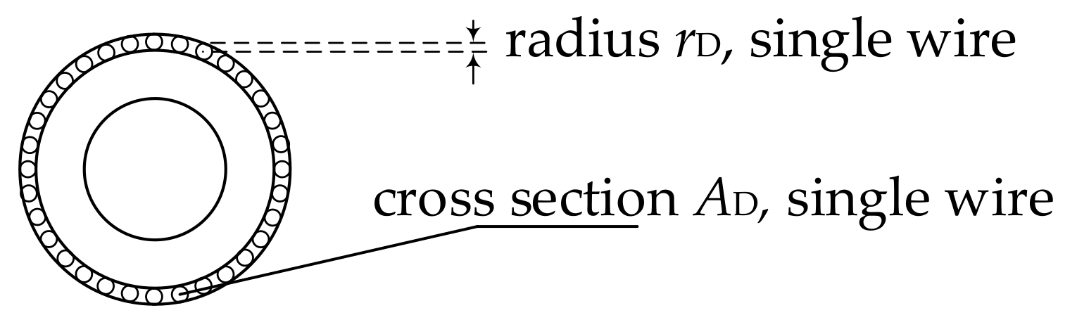
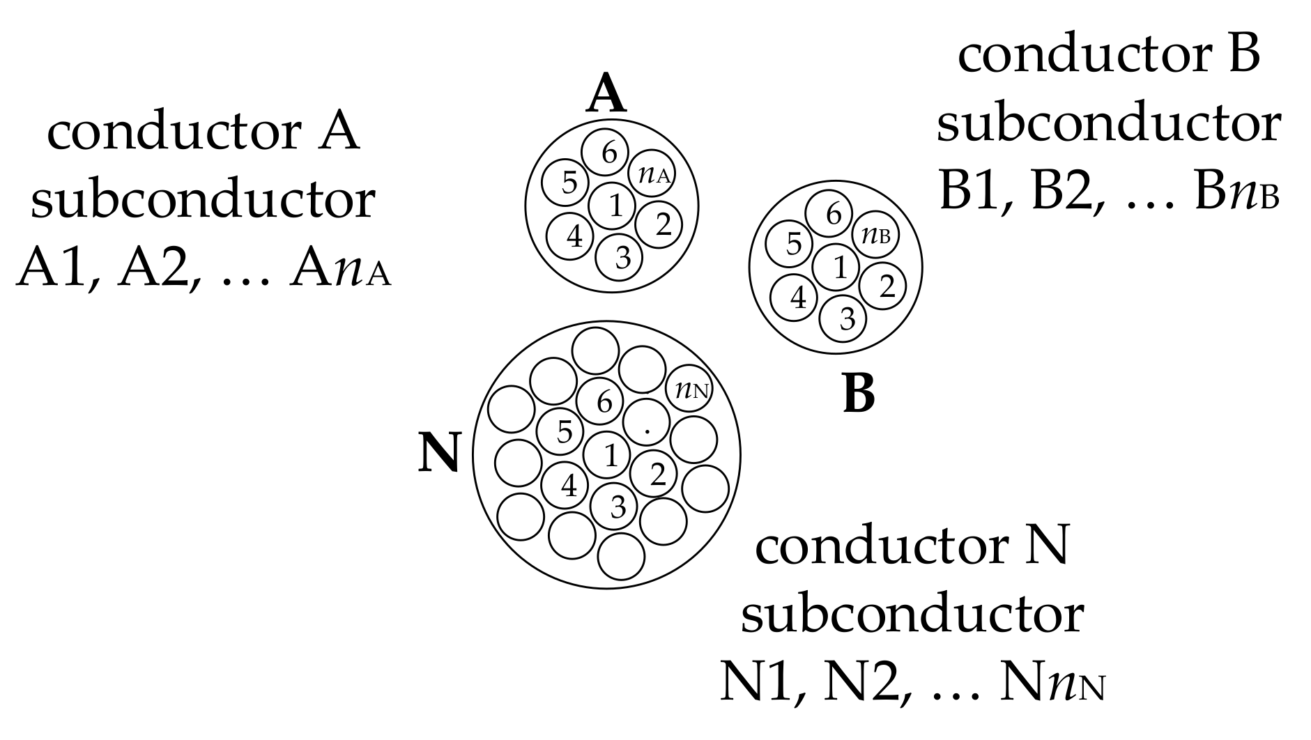
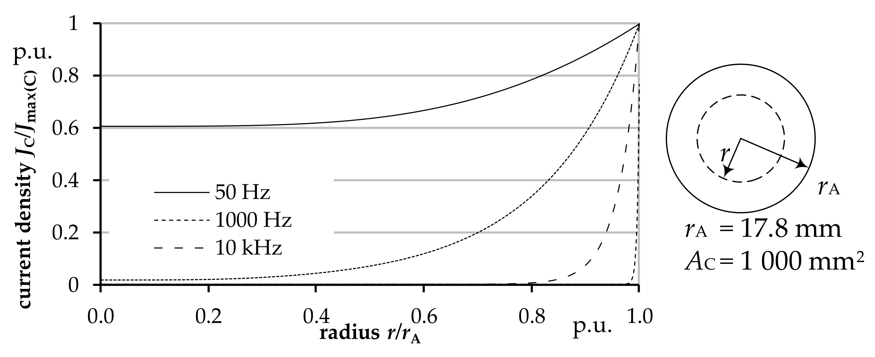
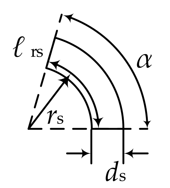
2.2. Partial Subconductor Method

The principle of the partial subconductor method as published by Comellini [26] is based on the segmentation of the conductor cross-sectional area into sufficiently small subconductors so that the current density will be nearly homogeneous within each subconductor. The subconductors of the system are inductively coupled through the mutual inductance per unit length $Z_{mn}^{\prime }$ of all conductor loops. Therefore, it is possible to model skin and proximity effects in the conductors of the cable and in the earth. Figure 4 shows the principle of segmentation.

The inductive coupling of current and voltage of all subconductors is characterized by the equation system of the subconductor-submatrices as specified in Equation (5) for three conductors $\mathrm{A}$, $\mathrm{B}$, and $\mathrm{C}$.

$$\left[\begin{array}{c}{{\underline{\mathit{v}}}^{\prime }}_{\mathbf{A}}\\ {{\underline{\mathit{v}}}^{\prime }}_{\mathbf{B}}\\ {{\underline{\mathit{v}}}^{\prime }}_{\mathbf{C}}\end{array}\right]=\left[\begin{array}{ccc}{{\underline{\mathit{Z}}}^{\prime }}_{\mathbf{AA}}& {{\underline{\mathit{Z}}}^{\prime }}_{\mathbf{AB}}& {{\underline{\mathit{Z}}}^{\prime }}_{\mathbf{AC}}\\ {{\underline{\mathit{Z}}}^{\prime }}_{\mathbf{BA}}& {{\underline{\mathit{Z}}}^{\prime }}_{\mathbf{BB}}& {{\underline{\mathit{Z}}}^{\prime }}_{\mathbf{BC}}\\ {{\underline{\mathit{Z}}}^{\prime }}_{\mathbf{CA}}& {{\underline{\mathbf{Z}}}^{\prime }}_{\mathbf{CB}}& {{\underline{\mathit{Z}}}^{\prime }}_{\mathbf{CC}}\end{array}\right]·\left[\begin{array}{c}{\underline{\mathit{i}}}_{\mathbf{A}}\\ {\underline{\mathit{i}}}_{\mathbf{B}}\\ {\underline{\mathit{i}}}_{\mathbf{C}}\end{array}\right]$$

(5)

It is possible to incorporate all conductors of the system into the algorithm, for instance any of the cable components such as the core conductor, shield, armor, earth, semiconducting layers and possible return conductors of the system. The conventional subconductor method realizes a “fixed” segmentation with arc segments. Dommel [27] discussed different shapes of segments, for instance circles, squares and so forth. The limitation to frequencies of $f<10\mathrm{kHz}$ is a significant disadvantage of the fixed segmentation. The reason for the limitation to frequencies is named by Lucas [28] described in detail in Schidt et al. [29,30]. The limitation of the conventional sub-conductor method can be avoided by using frequency-dependent segmentation.

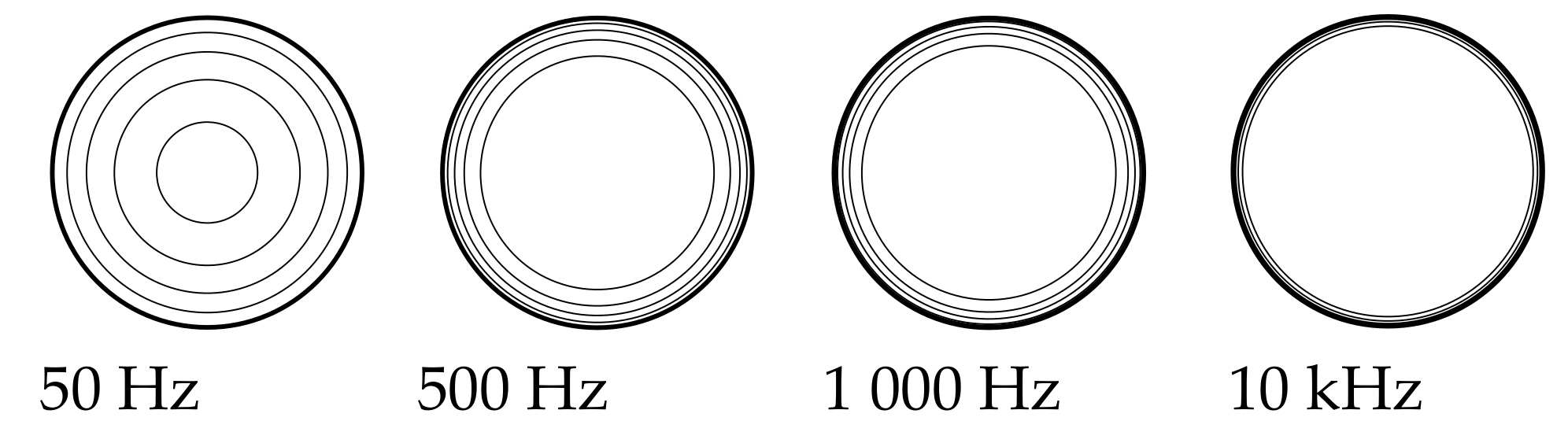
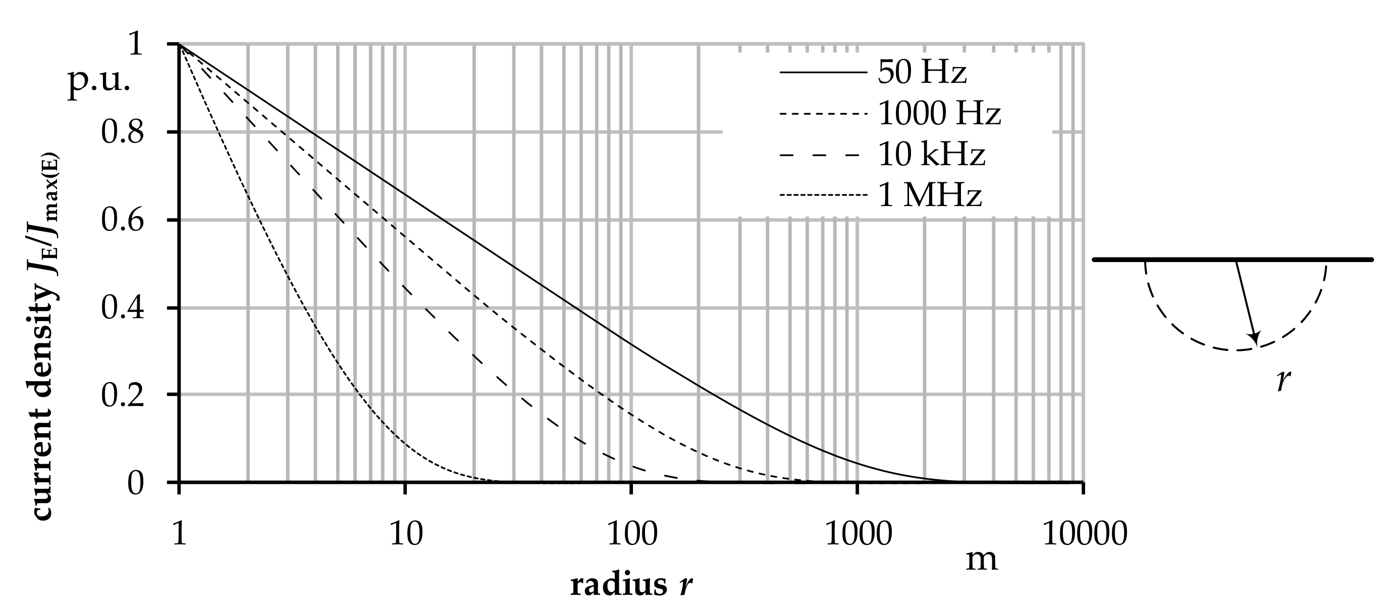
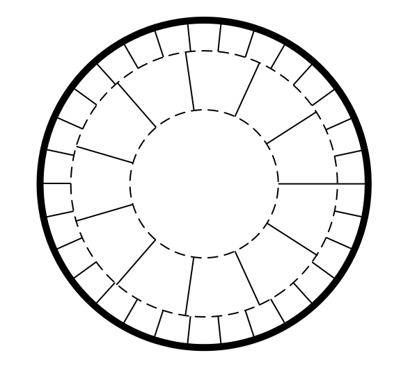
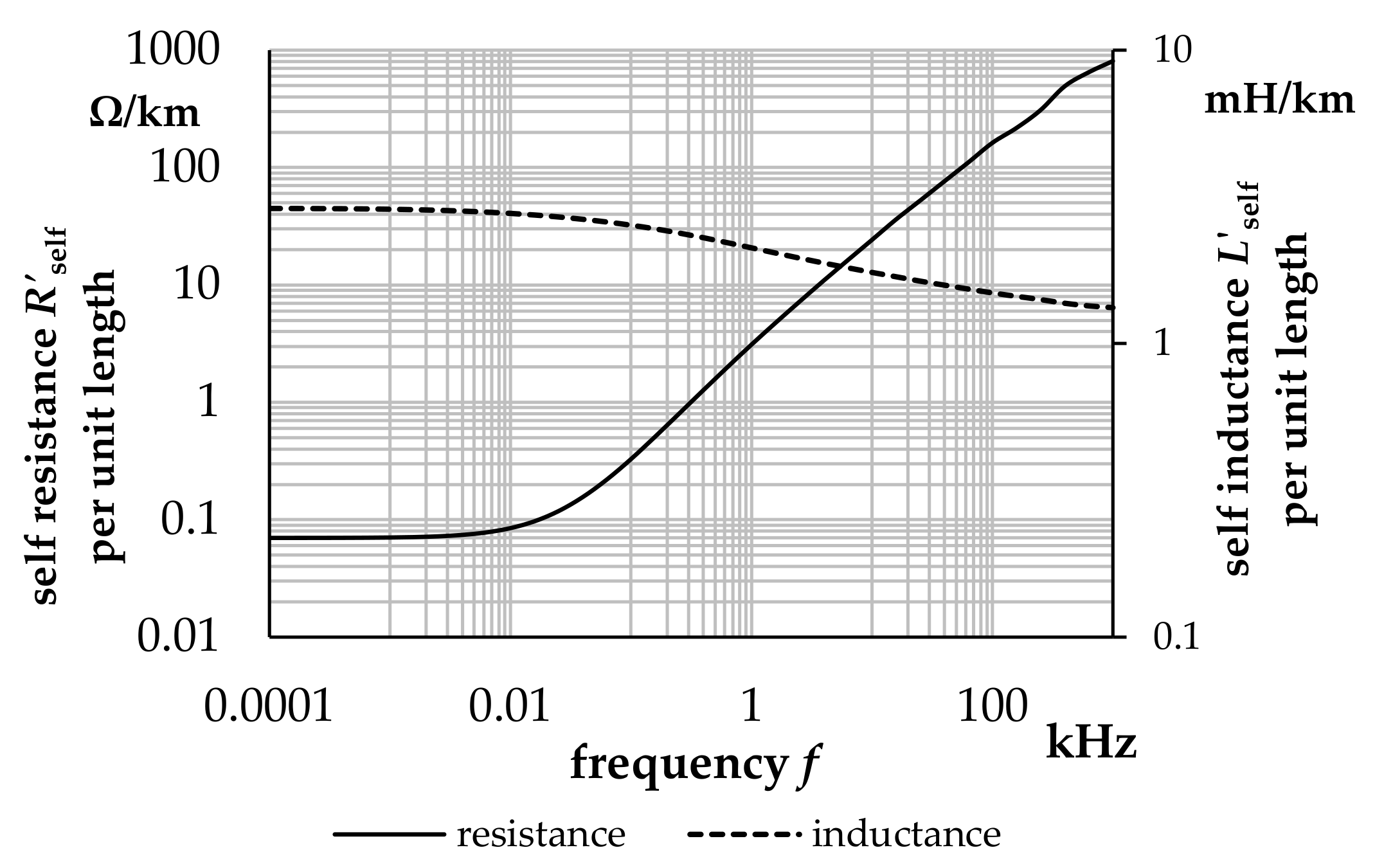
2.3. Frequency-Dependent Segmentation of Conductors

The segmentation of a cylindrical conductor is realized considering the skin and proximity effect. To determine the segmentation algorithm, the current density $J(f,r)$ of the cylindrical conductor is analytically derived from Maxwell’s equations as a function of the frequency f and the radius r. Figure 5 illustrates the current density $J_{\mathrm{C}}/J_{\text{max}}\left(\mathrm{C}\right)$ at different frequencies for a solid, cylindrical copper conductor with a cross-section area $A_{\mathrm{C}}$ of $1000{\mathrm{mm}}^2$.

With increasing frequency f the skin effect grows stronger. At high frequencies, a significant current flow remains directly under the surface only. For instance, at a frequency $f=1000\mathrm{Hz}$, $90\%$ of the current I is concentrated in the outer $4.5\mathrm{mm}$. Therefore, the cylindrical conductor is segmented across its radius $r_{\mathrm{A}}$ as a function of the relative current density $J/J_{\text{max}}$. It is assumed that a constant error of the current density distribution can be achieved by calculating the current density $J(f,r)$ with the outer radius of the i-th skin $r_i$ directly dependent on the relative current density $J/J_{\max }$. The number of skins n can be set in accordance to the required accuracy. Nevertheless, it must be considered that the number of skins impacts the algorithm’s computation time. The consideration of the proximity effect is covered by the skin subdivision into arc segments.

As an example, Figure 6 displays the allocation of the skins over the conductor’s radius exemplary for five skins. The determination of the skin radii $r_1$ to $r_n$ follows a $1/n$-increment of the relative current density $J/J_{\max }$. However, the subdivision of the conductors into skins as demonstrated in Figure 6 does not cover the proximity effect. This must be incorporated by another subdivision of the skins into arc segments (see Figure 7). Arnold [31] yields an analytical approach to calculate the proximity effect. Based on the error which occurs from the calculation of the subconductor impedances $Z_{mm}^{\prime }$ and $Z_{mn}^{\prime }$ , the segmentation of the skins can be defined. Nevertheless, calculating the mutual mean geometric distances $g_{mn}$ of two arc segments as indicated in Equation (2) and the self mean geometric distance $g_{mm}$ of one arc segment on itself as indicated in (3) causes a high numerical complexity. In order to simplify, Rees [25] and Brakelmann [32] introduced the centroid distance s of the corresponding arc segments into Expression (4), instead of using the mean geometric distance g. The replacement of the mean geometric distance g by the centroid distance s of the arc segments results in an error which cannot be ignored, but Rees [25] shows that at least for certain configurations it is essentially acceptable to use the centroid distance s. A numerical determination of the deviation between centroid distance s and mean geometric distance g is presented by Schmidt [29,30].

Those calculations have shown that for the geometric factors $k_{\mathrm{s}}={\ell }_{\mathrm{rs}}/d_{\mathrm{s}}$ smaller than 2, the relative deviation $s_{mn}/g_{mn}$ is minimized. Figure 8 gives an example for the segmentation into three skins for a frequency of $f=50\mathrm{Hz}$.

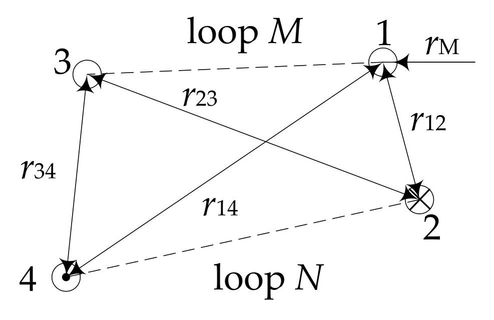
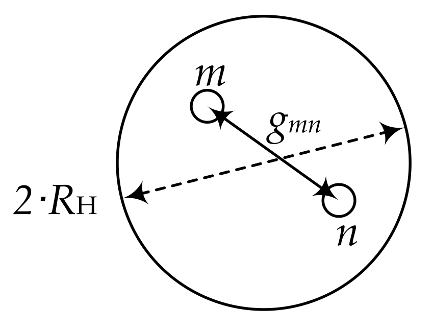
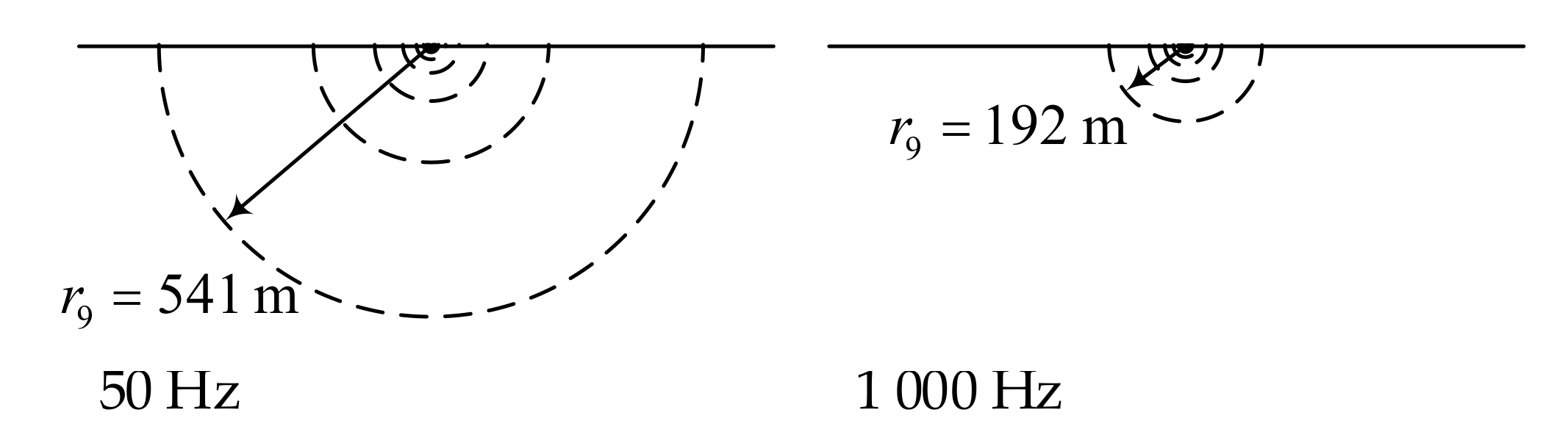
2.4. Earth Segmentation

The segmentation of the earth is based on the analytically calculated current distribution in the earth. The approach of Ruedenberg [33] can directly be applied to underground cable systems. The calculated current density $J_{\mathrm{E}}(f,r)$ is shown in Figure 9 and displays the relative current density $J_{\mathrm{E}}/J_{\max \left(\mathrm{E}\right)}$ as a function of the radius r at different frequencies between $50\mathrm{Hz}$ and $1\mathrm{MHz}$. The specific earth resistance ${\varrho }_{\mathrm{E}}$ is assumed to a typical value (in Central Europe) of $150\mathsf{\Omega }$ m.

The segmentation is again realized by analytical calculation of the conductor current density $J_{\mathrm{C}}/J_{\max }\left(\mathrm{C}\right)$. For frequencies of $f=50$ and $1000\mathrm{Hz}$, Figure 10 shows how ten skins would be allocated.

To provide a better overview, only every second skin is plotted in Figure 10. At the fictive hull cylinder with the radius $R_{\mathrm{H}}$ the current density J must have declined to zero. As Dommel [34] was able to demonstrate, this condition can be fulfilled for a distance of ten times the penetration depth ${\varrho }_{\mathrm{E}}$. The segmentation of the skins is done according to the results of the errors computation discussed in Schmidt [30].

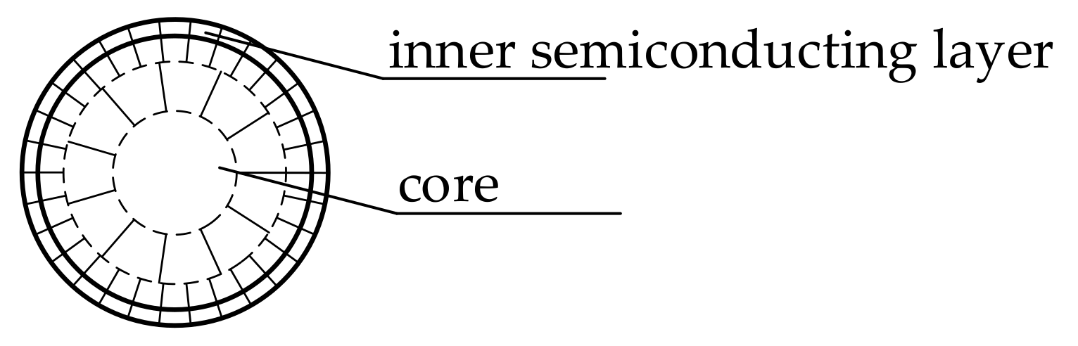
2.5. Shield Segmentation

The shields of single core cables are usually stranded rigid copper conductors illustrated in Figure 11.

In this case, the frequency-dependent segmentation is not necessary since the skin effect is only effective in single wires. The self-impedance per unit length of the single wire with the cross section $A_{\mathrm{D}}=\pi ·r_{\mathrm{D}}^2$ can be calculated by Equation (6).

$$\underline{Z}{}_{mm}^{\prime }=R_{\mathrm{ac}}^{\prime }\left(\mathrm{D}\right)+\mathrm{j}·\omega ·\frac{\mu }{2\pi }·ln\left(\frac{R_{\mathrm{H}}}{g_{mm}}\right)$$

(6)

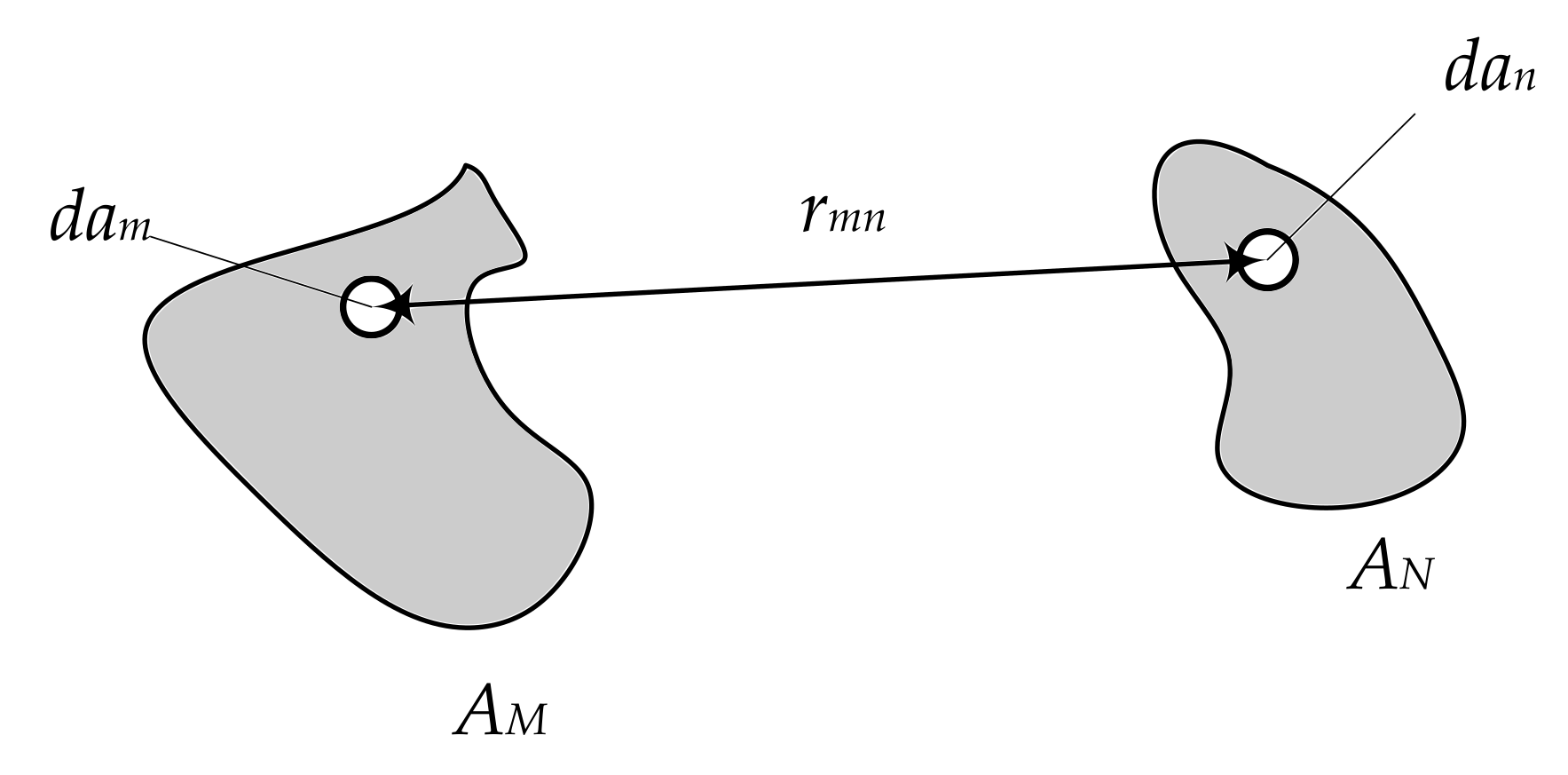
2.6. Calculation of Frequency-Dependent Impedances

Equation (4) describes the impedances ${\underline{Z}}^{\prime }$ of all subconductors in a certain area of all considered subconductors in a certain area and thus the inductive coupling between all subconductors. The reference conductor (or common return conductor) of all loops is the radius of the fictive hull cylinder $R_{\mathrm{H}}$. The complete impedance matrix of a system appears as represented in Equation (5) and contains the subconductor matrices of each individual phase. The rank of the impedance matrix ${\underline{\mathit{Z}}}^{\prime }$ is equal to the number of all subconductors in the enclosed area $n_{\mathrm{all}}$. A resistive component $R^{\prime }$, which characterizes the direct current resistance per unit length $R_m^{\prime }$ of the electrical subconductor m as a function of the specific resistance and the subconductor area $A_m$, is merely included in the self impedances $Z_{mm}^{\prime }$. The direct current resistances $R_m^{\prime }$ of all subconductors are comprised in a column vector ${\mathit{R}}^{\prime }$. The impedance matrix ${\underline{\mathit{Z}}}^{\prime }$ can be expressed according to Equation (7).

$${\underline{\mathit{Z}}}^{\prime }={\mathit{R}}^{\prime }+\mathrm{j}·\omega ·\frac{\mu }{2·\pi }·\left(ln{R}_{\mathrm{H}}-ln\mathit{s}\right)$$

(7)

The indices of the centroid distance elements in Matrix (8) designate the respective subconductor. The subscripted index names the m-th subconductor of the current-carrying loop and the superscripted index names the n-th subconductor influenced by the current-carrying loop.

$$\mathbf{s}=\left[\begin{array}{cccccccc}{s}_{\mathrm{A}1}^{\mathrm{A}1}& \cdots & s_{\mathrm{A}1}^{\mathrm{A}{n}_{\mathrm{A}}}& & & s_{\mathrm{A}1}^{N1}& \cdots & s_{\mathrm{A}1}^{N{n}_n}\\ ⋮& \ddots & ⋮& \cdots & \cdots & ⋮& \ddots & ⋮\\ s_{{\mathrm{A}n}_{\mathrm{A}}}^{\mathrm{A}1}& \cdots & s_{\mathrm{A}{n}_{\mathrm{A}}}^{\mathrm{A}{n}_A}& & & s_{\mathrm{A}{n}_{\mathrm{A}}}^{N1}& \cdots & s_{\mathrm{A}{n}_{\mathrm{A}}}^{N{n}_n}\\ & ⋮& & \ddots & & & ⋮& \\ & ⋮& & & \ddots & & ⋮& \\ s_{N1}^{\mathrm{A}1}& \cdots & s_{N1}^{\mathrm{A}{n}_{\mathrm{A}}}& & & s_{N1}^{N1}& \cdots & s_{N1}^{N{n}_n}\\ ⋮& & ⋮& \cdots & \cdots & ⋮& \ddots & ⋮\\ s_{N{n}_n}^{\mathrm{A}1}& \cdots & s_{N{n}_n}^{\mathrm{A}{n}_{\mathrm{A}}}& & & s_{N{n}_n}^{N1}& \cdots & s_{N{n}_n}^{N{n}_n}\end{array}\right]$$

(8)

The subconductor matrices of the centroid distances $s_{mn}$ and the admittance matrix ${\underline{\mathit{Y}}}^{\prime }$ are symmetrical. Therefore, to calculate the centroid distances s, it is sufficient to determine the elements above the main diagonal and to reflect them at the main diagonal. For unknown currents $\underline{\mathit{i}}$ of the cable system and known voltages ${\underline{\mathit{v}}}^{\prime }$, a system of equations (with reference to Equation (5)) can be obtained as given by Equation (9).

$$\underline{\mathit{i}}={\underline{\mathit{Y}}}^{\prime }·{\underline{\mathit{v}}}^{\prime }$$

(9)

The admittance matrix ${\underline{\mathit{Y}}}^{\prime }$ is the inverse of the impedance matrix ${\underline{\mathit{Z}}}^{\prime }$. The voltage across all subconductors in a conductor K is the same. It is:

$${\underline{V}}_K^{\prime }={\underline{V}}_{k1}^{\prime }={\underline{V}}_{k2}^{\prime }=\dots ={\underline{V}}_{k{n}_i}^{\prime }$$

(10)

The sum of the subconductor admittance matrices ${\underline{\mathit{Y}}}_{mn}^{\prime }$ and ${\underline{\mathit{Y}}}_{mm}^{\prime }$ can be realized using basic matrix operations demonstrated in Relation (11).

$${{\underline{\mathit{Y}}}^{\prime }}^{\mathrm{red}}=\mathit{T}·{\underline{\mathit{Y}}}^{\prime }·{\mathit{T}}^{-\mathbf{1}}$$

(11)

The dimension ($N\times n_{\mathrm{all}}$) of the transformation matrix $\mathit{T}$ is defined by the total number of conductors in the system N and the sum of all subconductors $n_{\mathrm{all}}$. Row K is associated with conductor K. All elements corresponding to the submatrix ${\mathit{Y}}_K^{\prime }$ are filled with 1, the remaining elements are filled with 0. For a seven-conductor system (3 × core, 3 × shield, 1 × earth) the transformation matrix $\mathit{T}$ is of the form indicated by Equation (12).

$$\mathbf{T}=\left[\begin{array}{cccc}{\mathbf{1}}_{(\mathbf{1}\mathbf{\times }{\mathbf{n}}_{\mathbf{A}})}& \mathbf{0}& \mathbf{0}& \mathbf{0}\\ \mathbf{0}& {\mathbf{1}}_{(\mathbf{1}\mathbf{\times }{\mathbf{n}}_{\mathbf{B}})}& \mathbf{0}& \mathbf{0}\\ \mathbf{0}& \mathbf{0}& {\mathbf{1}}_{(\mathbf{1}\mathbf{\times }{\mathbf{n}}_{\mathbf{C}})}& \mathbf{0}\\ \mathbf{0}& \mathbf{0}& \mathbf{0}& {\mathbf{1}}_{(\mathbf{1}\mathbf{\times }{\mathbf{n}}_{\mathbf{E}})}\end{array}\right]$$

(12)

The number of rows in the transformation matrix $\mathit{T}$ according to Equation (12) is equal to the number of conductors N. The number of elements per row represents the number of subconductors n in conductor K. The reduced impedance matrix ${{\underline{\mathit{Z}}}^{\prime }}^{\mathrm{red}}$ can be obtained from the reduced admittance matrix ${{\underline{\mathit{Y}}}^{\prime }}^{\mathrm{red}}$.

$${{\underline{\mathit{Z}}}^{\prime }}^{\mathrm{red}}={\left({{\underline{\mathit{Y}}}^{\prime }}^{\mathrm{red}}\right)}^{-1}$$

(13)

2.7. System Impedances

The reduced impedance matrix ${{\underline{\mathit{Z}}}^{\prime }}^{\mathrm{red}}$ (13) contains the submatrices of all conductors. It is useful to modify the matrix containing all submatrices to a ($6\times 6$) matrix. Expression (14) shows the structure of the reduced system with all submatrices for the core (C), shield (S) and earth (E).

$$\left[\begin{array}{c}{\underline{\mathit{v}}}_{\mathbf{C}}^{\prime }\\ {\underline{\mathit{v}}}_{\mathbf{S}}^{\prime }\\ {\underline{\mathit{v}}}_{\mathbf{E}}^{\prime }\end{array}\right]=\left[\begin{array}{ccc}{\underline{\mathit{Z}}}_{\mathbf{CC}}^{\prime }& {\underline{\mathit{Z}}}_{\mathbf{CS}}^{\prime }& {\underline{\mathit{Z}}}_{\mathbf{CE}}^{\prime }\\ {\underline{\mathit{Z}}}_{\mathbf{SC}}^{\prime }& {\underline{\mathit{Z}}}_{\mathbf{SS}}^{\prime }& {\underline{\mathit{Z}}}_{\mathbf{SE}}^{\prime }\\ {\underline{\mathit{Z}}}_{\mathbf{EC}}^{\prime }& {\underline{\mathit{Z}}}_{\mathbf{ES}}^{\prime }& {\underline{\mathit{Z}}}_{\mathbf{EE}}^{\prime }\end{array}\right]·\left[\begin{array}{c}{\underline{\mathit{i}}}_{\mathbf{C}}\\ {\underline{\mathit{i}}}_{\mathbf{S}}\\ {\underline{\mathit{i}}}_{\mathbf{E}}\end{array}\right]$$

(14)

The voltage vector ${\underline{\mathit{v}}}^{\prime }$ describes longitudinal voltages measured against the hull cylinder. The equation system (14) can be partitioned into impedances of the cable system and impedances of return conductors (15).

$$\left[\begin{array}{c}{{\underline{\mathit{v}}}^{\prime }}_{\mathbf{c}}^{\mathbf{p}}\\ {{\underline{\mathit{v}}}^{\prime }}_{\mathbf{e}}^{\mathbf{p}}\end{array}\right]=\left[\begin{array}{cc}{{\underline{\mathit{Z}}}^{\prime }}_{\mathbf{cc}}^{\mathbf{p}}& {{\underline{\mathit{Z}}}^{\prime }}_{\mathbf{ce}}^{\mathbf{p}}\\ {{\underline{\mathit{Z}}}^{\prime }}_{\mathbf{ec}}^{\mathbf{p}}& {{\underline{\mathit{Z}}}^{\prime }}_{\mathbf{ee}}^{\mathbf{p}}\end{array}\right]·\left[\begin{array}{c}{\underline{\mathit{i}}}_{\mathbf{c}}^{\mathbf{p}}\\ {\underline{\mathit{i}}}_{\mathbf{e}}^{\mathbf{p}}\end{array}\right]$$

(15)

The reference potential is the potential of the fictive hull cylinder $U_{\mathrm{H}}=0$. It can be expressed in Equation (16).

$$\begin{array}{cc}\hfill {{\underline{\mathit{v}}}^{\prime }}_{\mathbf{c}}^{\mathbf{p}}& ={{\underline{\mathit{Z}}}^{\prime }}_{\mathbf{cc}}^{\mathbf{p}}·{\underline{\mathit{i}}}_{\mathbf{c}}^{\mathbf{p}}+{{\underline{\mathit{Z}}}^{\prime }}_{\mathbf{ce}}^{\mathbf{p}}·{\underline{\mathit{i}}}_{\mathbf{e}}^{\mathbf{p}}\hfill \\ \hfill \mathbf{0}& ={{\underline{\mathit{Z}}}^{\prime }}_{\mathbf{el}}^{\mathbf{p}}·{\underline{\mathit{i}}}_{\mathbf{c}}^{\mathbf{p}}+{{\underline{\mathit{Z}}}^{\prime }}_{\mathbf{ee}}^{\mathbf{p}}·{\underline{\mathit{i}}}_{\mathbf{e}}^{\mathbf{p}}\hfill \end{array}$$

(16)

Equation (16) can be rearranged to obtain (17) for the current ${\underline{\mathit{i}}}_{\mathbf{e}}^{\mathbf{p}}$:

$${\underline{\mathit{i}}}_{\mathbf{e}}^{\mathbf{p}}={\left({{-\underline{\mathit{Z}}}^{\prime }}_{\mathbf{ee}}^{\mathbf{p}}\right)}^{-1}·\left({{\underline{\mathit{Z}}}^{\prime }}_{\mathbf{ec}}^{\mathbf{p}}\right)·{\underline{\mathit{i}}}_{\mathbf{c}}^{\mathbf{p}}$$

(17)

Inserting Equation (17) into (16) results in Equation (18) for the voltage ${{\underline{\mathit{u}}}^{\prime }}_{\mathbf{c}}^{\mathbf{p}}$.

$$\begin{array}{cc}\hfill {{\underline{\mathit{u}}}^{\prime }}_{\mathbf{c}}^{\mathbf{p}}& =({{\underline{\mathit{Z}}}^{\prime }}_{\mathbf{cc}}^{\mathbf{p}}-{{\underline{\mathit{Z}}}^{\prime }}_{\mathbf{ce}}^{\mathbf{p}}·{\left({{\underline{\mathit{Z}}}^{\prime }}_{\mathbf{ee}}^{\mathbf{p}}\right)}^{-1}·{{\underline{\mathit{Z}}}^{\prime }}_{\mathbf{ec}}^{\mathbf{p}})·{\underline{\mathit{i}}}_{\mathbf{c}}^{\mathbf{p}}\hfill \\ \hfill {{\underline{\mathit{u}}}^{\prime }}_{\mathbf{c}}^{\mathbf{p}}& ={{\underline{\mathit{Z}}}^{\prime }}_{\mathbf{mod}}·{\underline{\mathit{u}}}_{\mathbf{c}}^{\mathbf{p}}\hfill \end{array}$$

(18)

The modified matrix ${{\underline{\mathit{Z}}}^{\prime }}_{\mathbf{mod}}$ has the rank of the sum of all cable conductors. The matrix is a ($6\times 6$) matrix single core cable system (3 × core, 3 × shield). It is also possible to reduce the coefficient matrix of equation system (14) to a ($3\times 3$) matrix. In case of earthed shields on both cable ends, the return conductor submatrices of the partitioned matrix (15) contains the shield submatrices. The earth and shield influence is considered in all modified impedance matrices ${\underline{\mathit{Z}}}_{\mathbf{mod}}^{\prime }$. In principle, this approach can also be realized for one-sided shield earthing (Schmidt [30]).

2.8. Impact of Semiconducting Layers

The influence of semiconducting layers is formulated in only very few publications. Ametani [35] determined the impact of semiconducting layers by modifying Schelkunoff’s method [5]. Semiconducting layers can also be considered with the subconductor method. A one-skin segmentation for the inner semiconducting layer is shown in Figure 12.

Segmentation can be realized also with more than one skin. The specific resistances of semiconducting layers can be ${\varrho }_{\mathrm{sl}}=0.01\dots 10\mathsf{\Omega }$ m according to Ametani [35]. Nevertheless, cable manufacturers specify particular values between ${\varrho }_{\mathrm{sl}}=10$ and $100\mathsf{\Omega }$ m. The calculated resistance per unit length $R_{\mathrm{ac}\left(\mathrm{C}\right)}^{\prime }$ for relevant specific semiconducting layer resistances ${\varrho }_{\mathrm{sl}}$ is shown in Figure 13.

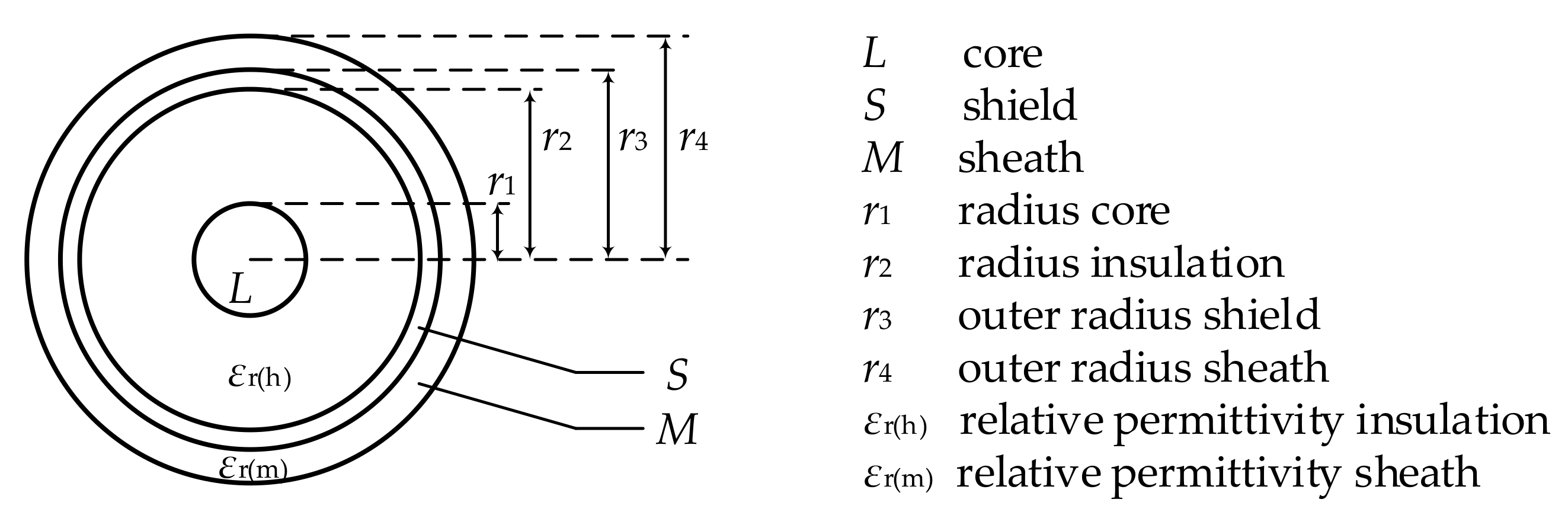
2.9. Main Insulation Capacitance

The single core cable capacitance shown in Figure 14 can be calculated by Equation (19) for the cross-linked polyethylene (XLPE) main insulation $C_{\mathrm{CS}}^{\prime }$:

$$C_{\mathrm{CS}}^{\prime }=2·\pi ·{\epsilon }_0·{\epsilon }_{\mathrm{r}\left(\mathrm{h}\right)}·\frac{1}{ln\left(\frac{r_2}{r_1}\right)}$$

(19)

and for the sheath capacitance $C_{\mathrm{sh}}^{\prime }$ (20).

$$C_{\mathrm{sh}}^{\prime }=2·\pi ·{\epsilon }_0·{\epsilon }_{\mathrm{r}\left(\mathrm{m}\right)}·\frac{1}{ln\left(\frac{r_4}{r_3}\right)}$$

(20)

The capacitances depend on the cylinder geometry, the relative permittivity ${\epsilon }_{\mathrm{r}}$ of the insulation and the polarization. The frequency-dependent effects of polarization are investigated in several publications (Liu [36], Hadid and Schmidt [37]). The frequency range of polarization types are given in

Table 1. Frequency ranges of polarization.

Polarization	Frequency Range ${\mathit{f}}_{\mathbf{e}}$
Electronic	≈${10}^{15}\mathrm{Hz}$
Ionic	≈${10}^{12}\mathrm{Hz}$
Orientational	≈${10}^9\mathrm{Hz}$
Interfacial	$\mathrm{mHz}\dots \mathrm{kHz}$

(see also Liu [36]).

The table shows that electronic, ionic, and orientational polarization will not contribute significantly to the capacitances of single core cables. A typical interfacial polarization occurs between the XLPE insulation and the semiconducting layers. This effect is of relevance in a frequency range $f\le 1\mathrm{Hz}$. The interfacial polarization can be ignored in frequency ranges $f\ge 10\mathrm{Hz}$. Therefore, the frequency dependency of the capacitances can be generally neglected in an algorithm for frequency-dependent parameters. A typical interfacial polarization occurs between the XLPE insulation and the semiconducting

layers. This effect is of relevance in a frequency range $f\le 1\mathrm{Hz}$. The interfacial polarization can be ignored in frequency ranges $f\ge 10\mathrm{Hz}$. Therefore, the frequency dependency of the capacitances can be generally neglected in an algorithm for frequency-dependent parameters. The semiconducting layers have an influence on the capacitance $C_{\mathrm{CS}}^{\prime }$, but for transient calculations it can be neglected. Hadid and Schmidt [37] and Wagenaars [38] confirm this approach.

2.10. Sheath Capacitances

2.10.1. Earth Installation

Ametani [1], Wedepohl [2], Gustavsen [39], and Marti L. [13] neglected the earth resistance $R_{\mathrm{E}}$ and the earth capacitance $C_{\mathrm{E}}$. In Schmidt [30], this approach is confirmed for specific earth resistances ${\varrho }_{\mathrm{E}}<500\mathsf{\Omega }\mathrm{m}$ and frequencies $f<100\mathrm{kHz}$. The sheath capacitance per unit length $C_{\mathrm{sh}}^{\prime }$ can be calculated with Equation (20).

2.10.2. Air Installation

For correct calculation of shield-shield capacitance $C_{\mathrm{SS}}$, the sheath capacitance $C_{\mathrm{sh}}$ and the air capacitance $C_{\mathrm{E}}$ have to be considered. The sheath capacitance $C_{\mathrm{sh}}$ is significantly larger than the air capacitance $C_{\mathrm{E}}$. Therefore, the sheath capacitance $C_{\mathrm{sh}}$ can be neglected (Schmidt [30]). This is also valid in case of small phase distances. The sheath capacitance $C_{\mathrm{sh}}$ can be calculated with the charge simulation methods of Steinbigler [40], and Probst [41].

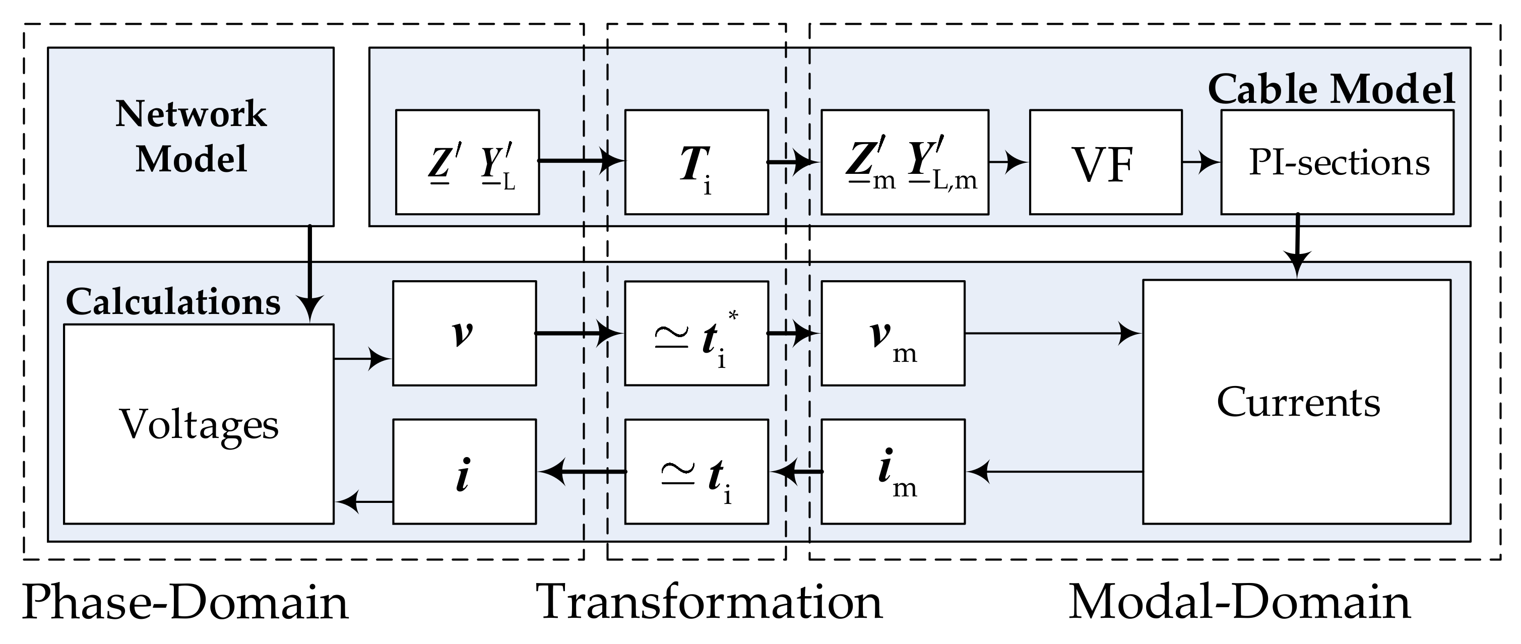
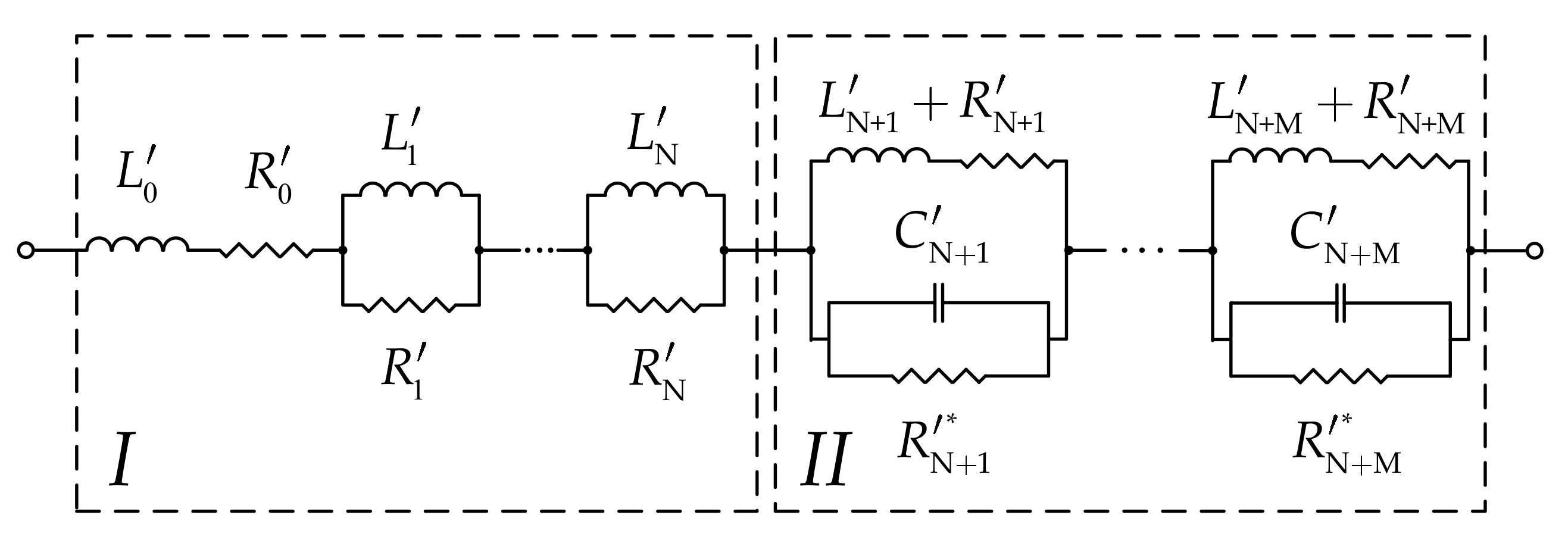
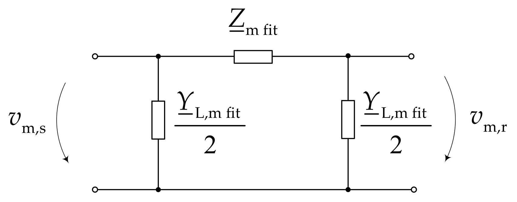
3. Wave Propagation Model

3.1. Approach

The wave propagation in a multi-conductor cable or transmission line can be represented in the frequency domain with second-order differential equations from Marti J. [42]:

$$\frac{{\mathrm{d}}^2\underline{\mathit{V}}}{\mathrm{d}{x}^2}={\underline{\mathit{Z}}}^{\prime }{\underline{\mathit{Y}}}_{\mathrm{L}}^{\prime }\underline{\mathit{V}}$$

(21)

$$\frac{{\mathrm{d}}^2\underline{\mathit{I}}}{\mathrm{d}{x}^2}={\underline{\mathit{Y}}}_{\mathrm{L}}^{\prime }{\underline{\mathit{Z}}}^{\prime }\underline{\mathit{I}}$$

(22)

The longitudinal impedances in the phase domain ${\underline{\mathit{Z}}}^{\prime }$ are calculated using the partial subconductor method as in Equation (7). The shunt admittance in the phase domain ${\underline{\mathit{Y}}}_{\mathrm{L}}^{\prime }$ represents the capacitance equations given in Equations (19) and (20). The index “L” stands for lateral. In order to solve the differential Equations (21) and (22), a modal transformation technique has been proposed in Marti J. [42]. As a result, the coupling between the cable conductors disappears and the cable system can be considered as decoupled single conductors. In the modal domain, the Equations (21) and (22) can be rewritten as:

$$\frac{{\mathrm{d}}^2{\underline{\mathit{V}}}_{\mathrm{m}}}{\mathrm{d}{x}^2}={\underline{\mathit{T}}}_{\mathrm{v}}^{-1}{\underline{\mathit{Z}}}^{\prime }{\underline{\mathit{Y}}}_{\mathrm{L}}^{\prime }{\underline{\mathit{T}}}_{\mathrm{v}}{\underline{\mathit{V}}}_{\mathrm{m}}=\underline{\mathit{\lambda }}{\underline{\mathit{V}}}_{\mathrm{m}}$$

(23)

$$\frac{{\mathrm{d}}^2{\underline{\mathit{I}}}_{\mathrm{m}}}{\mathrm{d}{x}^2}={\underline{\mathit{T}}}_{\mathrm{i}}^{-1}{\underline{\mathit{Y}}}_{\mathrm{L}}^{\prime }{\underline{\mathit{Z}}}^{\prime }{\underline{\mathit{T}}}_{\mathrm{i}}{\underline{\mathit{I}}}_{\mathrm{m}}=\underline{\mathit{\lambda }}{\underline{\mathit{I}}}_{\mathrm{m}}$$

(24)

where $\underline{\mathit{\lambda }}$ is a diagonal matrix which represents the eigenvalues matrix of ${\underline{\mathit{Z}}}^{\prime }$ ${\underline{\mathit{Y}}}_{\mathrm{L}}^{\prime }$ and ${\underline{\mathit{Y}}}_{\mathrm{L}}^{\prime }$${\underline{\mathit{Z}}}^{\prime }$. For the transformation into modal domain the modal transformation matrices ${\underline{\mathit{T}}}_{\mathrm{i}}$ and ${\underline{\mathit{T}}}_{\mathrm{v}}$ are used. The relation between the matrices is given by Marti J. [13]:

$${\underline{\mathit{T}}}_{\mathrm{v}}={\left[{\underline{\mathit{T}}}_{\mathrm{i}}^{-1}\right]}^{\mathrm{tr}}$$

(25)

Therefore, it is sufficient to calculate only one of them. In this paper, the results for ${\underline{\mathit{T}}}_{\mathrm{i}}$ will be calculated as in Chrysochos et al. [43].

In order to make the calculation in the modal domain, the quantities ${\underline{\mathit{Z}}}^{\prime }$, ${\underline{\mathit{Y}}}_{\mathrm{L}}^{\prime }$, $\underline{\mathit{V}}$ and $\underline{\mathit{I}}$ have to be transformed into this domain. From Equations (23) and (24), it can be derived:

$${\underline{\mathit{T}}}_{\mathrm{v}}^{-1}{\underline{\mathit{Z}}}^{\prime }{\underline{\mathit{Y}}}_{\mathrm{L}}^{\prime }{\underline{\mathit{T}}}_{\mathrm{v}}=\underline{\mathit{\lambda }}$$

(26)

$${\underline{\mathit{T}}}_{\mathrm{i}}^{-1}{\underline{\mathit{Y}}}_{\mathrm{L}}^{\prime }{\underline{\mathit{Z}}}^{\prime }{\underline{\mathit{T}}}_{\mathrm{i}}=\underline{\mathit{\lambda }}$$

(27)

With simple matrix perturbation, the above equations are then rewritten as:

$${\underline{\mathit{T}}}_{\mathrm{v}}^{-1}{\underline{\mathit{Z}}}^{\prime }\left({\underline{\mathit{T}}}_{\mathrm{i}}{\underline{\mathit{T}}}_{\mathrm{i}}^{-1}\right){\underline{\mathit{Y}}}_{\mathrm{L}}^{\prime }{\underline{\mathit{T}}}_{\mathrm{v}}=\underline{\mathit{\lambda }}$$

(28)

$${\underline{\mathit{T}}}_{\mathrm{i}}^{-1}{\underline{\mathit{Y}}}_{\mathrm{L}}^{\prime }\left({\underline{\mathit{T}}}_{\mathrm{v}}{\underline{\mathit{T}}}_{\mathrm{v}}^{-1}\right){\underline{\mathit{Z}}}^{\prime }{\underline{\mathit{T}}}_{\mathrm{i}}=\underline{\mathit{\lambda }}$$

(29)

By rearranging the terms and by using the Equation (25) in (28) and (29), the longitudinal impedance and the shunt admittance in the modal domain can be defined as:

$${\underline{\mathit{Z}}}_{\mathrm{m}}^{\prime }={\underline{\mathit{T}}}_{\mathrm{i}}^{\mathrm{tr}}{\underline{\mathit{Z}}}^{\prime }{\underline{\mathit{T}}}_{\mathrm{i}}$$

(30)

$${\underline{\mathit{Y}}}_{\mathrm{L},\mathrm{m}}^{\prime }={\underline{\mathit{T}}}_{\mathrm{i}}^{-1}{\underline{\mathit{Y}}}_{\mathrm{L}}^{\prime }{\left[{\underline{\mathit{T}}}_{\mathrm{i}}^{-1}\right]}^{\mathrm{tr}}$$

(31)

Both matrices in Equations (30) and (31) are diagonal. The frequency dependence of the elements of ${\underline{\mathit{Y}}}_{\mathrm{L},\mathrm{m}}^{\prime }$ cannot be neglected (as assumed for the elements of ${\underline{\mathit{Y}}}_{\mathrm{L}}^{\prime }$). This is related to the frequency dependent elements of ${\underline{\mathit{T}}}_{\mathrm{i}}$. The elements of ${\underline{\mathit{Z}}}_{\mathrm{m}}^{\prime }$ are also strongly frequency-dependent. In order to take the frequency dependency of ${\underline{\mathit{Z}}}_{\mathrm{m}}^{\prime }$ and ${\underline{\mathit{Y}}}_{\mathrm{L},\mathrm{m}}^{\prime }$ into account, their diagonal elements need to be approximated by mathematical functions using the vector fitting algorithm (VF) of Gustavsen and Semlyen [15], and Gustavsen [16]. For example, the first diagonal element in ${\underline{\mathit{Z}}}_{\mathrm{m}}^{\prime }$ can be approximated using VF as:

$$\begin{array}{ll}{\underline{Z}}_{\mathrm{m}\mathrm{fit}}^{\prime }& =d+\mathrm{j}\omega h+{\displaystyle \sum _{\mathrm{q}=1}^{\mathrm{N}}}\frac{p_{\mathrm{q}}}{\mathrm{j}\omega -a_{\mathrm{q}}}\\ & +{\displaystyle \sum _{\mathrm{b}=\mathrm{N}+1}^{\mathrm{N}+\mathrm{M}}}\left(\frac{s_{\mathrm{b},\mathrm{re}}+\mathrm{j}{s}_{\mathrm{b},\mathrm{im}}}{\mathrm{j}\omega +g_{\mathrm{b},\mathrm{re}}-\mathrm{j}{g}_{\mathrm{b},\mathrm{im}}}+\frac{s_{\mathrm{b},\mathrm{re}}-\mathrm{j}{s}_{\mathrm{b},\mathrm{im}}}{\mathrm{j}\omega +g_{\mathrm{b},\mathrm{re}}+\mathrm{j}{g}_{\mathrm{b},\mathrm{im}}}\right)\end{array}$$

(32)

The accuracy of ${\underline{Z}}_{\mathrm{m}\mathrm{fit}}^{\prime }$ depends on the number of the real terms N and the number of the complex terms M. ${\underline{Z}}_{\mathrm{m}\mathrm{fit}}^{\prime }$ can be reproduced with an electrical network. In Hoshmeh et al. [21], an RL network has been used. Using such a network allows us to employ only the real poles and residues in the approximation (the complex terms are discarded). Although the fitting is achieved with a low order of approximation, the accuracy is affected. In this paper, an RLC network shown in Figure 15 is introduced with regards to all the poles and residues in the approximation including the complex terms.

As can be seen, the network has been divided into two sections. The elements of section I can be evaluated in a similar way as in Hoshmeh et al. [21]. The elements of section II are obtained as follows:

$$\begin{array}{l}\left.\begin{array}{c}{R}_{\mathrm{b}}^{\prime }={\displaystyle \frac{-2g_{\mathrm{b},\mathrm{re}}{s}_{\mathrm{b},\mathrm{re}}^3-2s_{\mathrm{b},\mathrm{re}}^2{s}_{\mathrm{b},\mathrm{im}}{g}_{\mathrm{b},\mathrm{im}}}{g_{\mathrm{b},\mathrm{im}}^2(s_{\mathrm{b},\mathrm{re}}^2+s_{\mathrm{b},\mathrm{im}}^2)}}\hfill \\ L_{\mathrm{b}}^{\prime }={\displaystyle \frac{2s_{\mathrm{b},\mathrm{re}}^3}{g_{\mathrm{b},\mathrm{im}}^2(s_{\mathrm{b},\mathrm{re}}^2+s_{\mathrm{b},\mathrm{im}}^2)}}\hfill \\ C_{\mathrm{b}}^{\prime }={\displaystyle \frac{1}{2s_{\mathrm{b},\mathrm{re}}}}\hfill \\ R_{\mathrm{b}}^{\prime *}={\displaystyle \frac{2s_{\mathrm{b},\mathrm{re}}^2}{g_{\mathrm{b},\mathrm{im}}{s}_{\mathrm{b},\mathrm{im}}-g_{\mathrm{b},\mathrm{re}}{s}_{\mathrm{b},\mathrm{re}}}}\hfill \end{array}\right\}\mathrm{b}=\mathrm{N}+1\dots \mathrm{N}+\mathrm{M}\end{array}$$

(33)

The first diagonal element of ${\underline{Y}}_{\mathrm{L},\mathrm{m}}^{\prime }$ is similarly approximated. Furthermore, $R_0^{\prime }$ and $L_0^{\prime }$ are assumed to be zeros in ${\underline{\mathit{Y}}}_{\mathrm{L},\mathrm{m}\mathrm{fit}}^{\prime }$. After calculating ${\underline{Z}}_{\mathrm{m}\mathrm{fit}}^{\prime }$ and ${\underline{Y}}_{\mathrm{L},\mathrm{m}\mathrm{fit}}^{\prime }$, they will be combined to form a developed PI section. Figure 16 shows a representation for the developed PI section after regarding the cable length, where $v_{\mathrm{m},\mathrm{s}}$ and $v_{\mathrm{m},\mathrm{r}}$ are the voltages in the modal domain at the sending and receiving ends, respectively. One single conductor in the developed cable model can then be represented by cascading a number of PI sections.

For the remaining diagonal elements of ${\underline{\mathit{Z}}}_{\mathrm{m}}^{\prime }$ and ${\underline{\mathit{Y}}}_{\mathrm{L},\mathrm{m}}^{\prime }$, the same procedure is used to form the other conductors in the developed cable model. From the Equations (23)–(25), the voltages and the currents are transformed into the modal domain as follows:

$${\underline{\mathit{V}}}_{\mathrm{m}}={\underline{\mathit{T}}}_{\mathrm{i}}^{\mathrm{tr}}\underline{\mathbf{V}}$$

(34)

$${\underline{\mathit{I}}}_{\mathrm{m}}={\underline{\mathit{T}}}_{\mathrm{i}}^{-1}\underline{\mathit{I}}$$

(35)

Equations (34) and (35) are still in the frequency domain. However, since the simulations in the power system are necessary in the time domain, these equations have to be transformed into this domain. For the voltages in the Equation (34), the convolution integral is applied as:

$${\mathit{v}}_{\mathrm{m}}(t\ast u)={\int }_{-\infty }^{\infty }{\mathit{t}}_{\mathrm{i}}^{*}(t-u)\mathit{v}\left(u\right)\mathrm{d}u$$

(36)

Evaluation this integral point by point is time consuming. By approximating the elements of ${\underline{\mathit{T}}}_{\mathrm{i}}^{\mathrm{tr}}$ using rational functions, an efficient recursive convolution method is used from Marti J. [12] and the above integral can be rewritten as a sum of exponentials:

$${\mathit{v}}_{\mathrm{m}}(t\ast u)={\int }_{\tau }^{\infty }b{\mathrm{e}}^{-l(u-\tau )}\mathit{v}\left(u\right)\mathrm{d}u$$

(37)

where b and l are the approximations parameters of the rational functions. The wave travel time $\tau$ for the impulse from one end of the cable to the other one is related to the imaginary term of the propagation function $\underline{\gamma }$:

$$\underline{\gamma }=\sqrt{{\underline{\mathit{Z}}}^{\prime }{\underline{\mathit{Y}}}_{\mathrm{L}}^{\prime }}$$

(38)

The voltage vector ${\mathit{v}}_{\mathrm{m}}\left(t\right)$ is calculated recursively from ${\mathit{v}}_{\mathrm{m}}(t-\Delta t)$ as:

$${\mathit{v}}_{\mathrm{m}}\left(t\right)=a_1{\mathit{v}}_{\mathrm{m}}(t-\Delta t)+a_2\mathit{v}(t-\tau )+a_3\mathit{v}(t-\tau -\Delta t)$$

(39)

In this relation, $a_1$, $a_2$ and $a_3$ are constants that mainly depend on b, l and $\Delta t$ Marti J. [42]. The same procedure is used to transform the currents in the Equation (35) into the time domain. In order to execute the time domain simulations, the differential equations for single conductors in the developed cable model have to be formulated. As shown in Hoshmeh et al. [21], the differential equations can be represented using state space techniques. A numerical backward Euler rule of integration can then be applied to find the solution for the related state space equations of Meyer and Dommel [44]. To solve the cable equations with the rest of the network, which is always defined in phase quantities, the calculated voltages and currents in the modal domain must be transformed back to phase quantities.

Figure 17 shows an overview for the realization of the 3PPI model. Starting from defining ${\underline{\mathit{Z}}}^{\prime }$ and ${\underline{\mathit{Y}}}_{\mathrm{L}}^{\prime }$, the cable model part is executed only once to provide the PI sections for the calculation part. In this part, the computation is evaluated every $\Delta t$. For the first one, the vector of the voltages $\mathit{v}$ is calculated using the network model and the vector of the currents $\mathit{i}$. By applying the recursive convolution between $\mathit{v}$ and the approximation of ${\mathit{t}}_{\mathrm{i}}^{*}$ ($\simeq {\mathit{t}}_{\mathrm{i}}^{*}$), the vector of the voltages ${\mathit{v}}_{\mathrm{m}}$ is calculated. Using the PI sections and ${\mathit{v}}_{\mathrm{m}}$, the state space equations are formulated and solved by means of numerical backward Euler rule of integration to yield the current vector ${\mathit{i}}_{\mathrm{m}}$. The recursive convolution between ${\mathit{i}}_{\mathrm{m}}$ and the approximation of ${\mathit{t}}_{\mathrm{i}}$ ($\simeq {\mathit{t}}_{\mathrm{i}}$) provides the vector of currents $\mathit{i}$ for the next $\Delta t$.

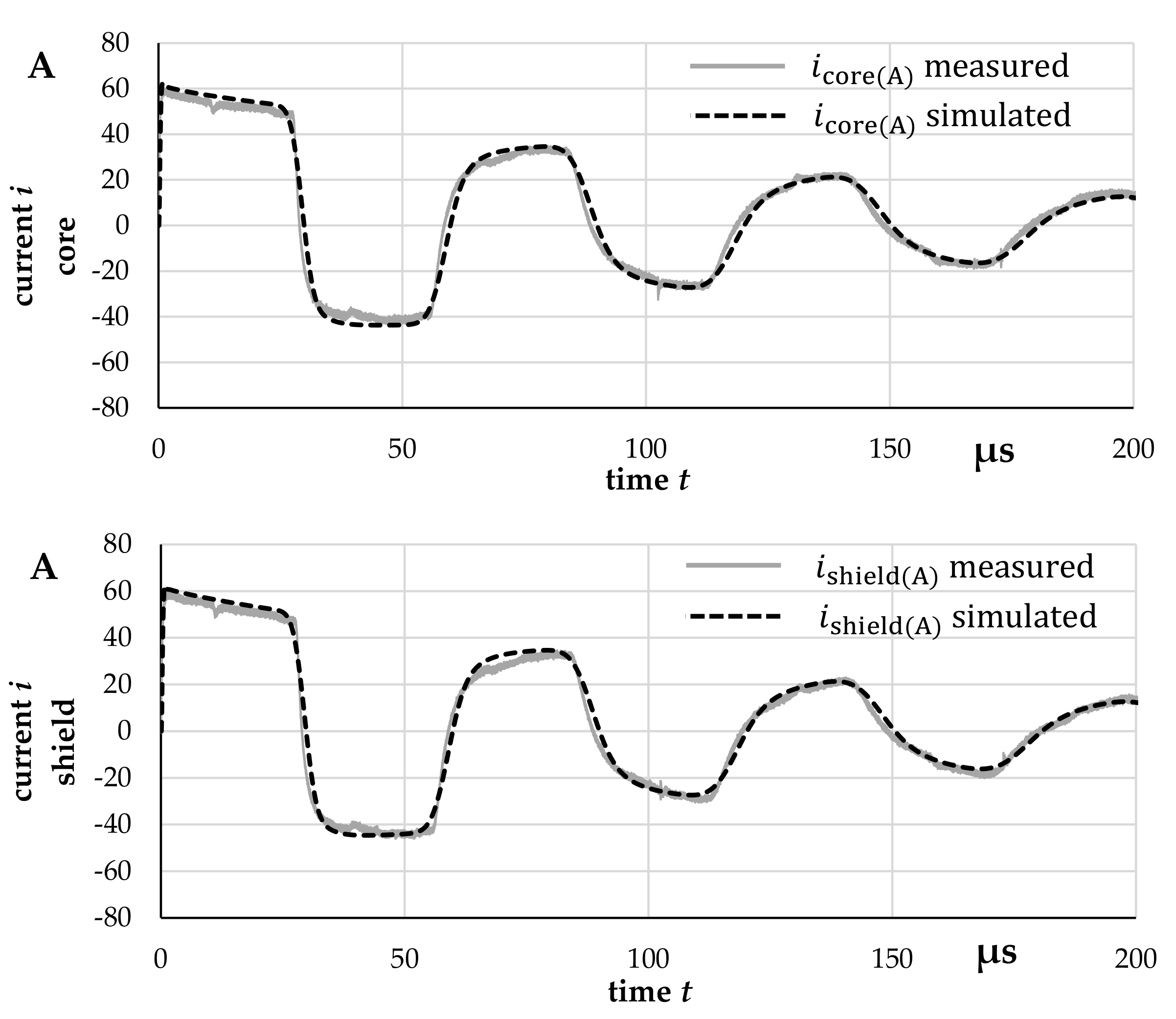
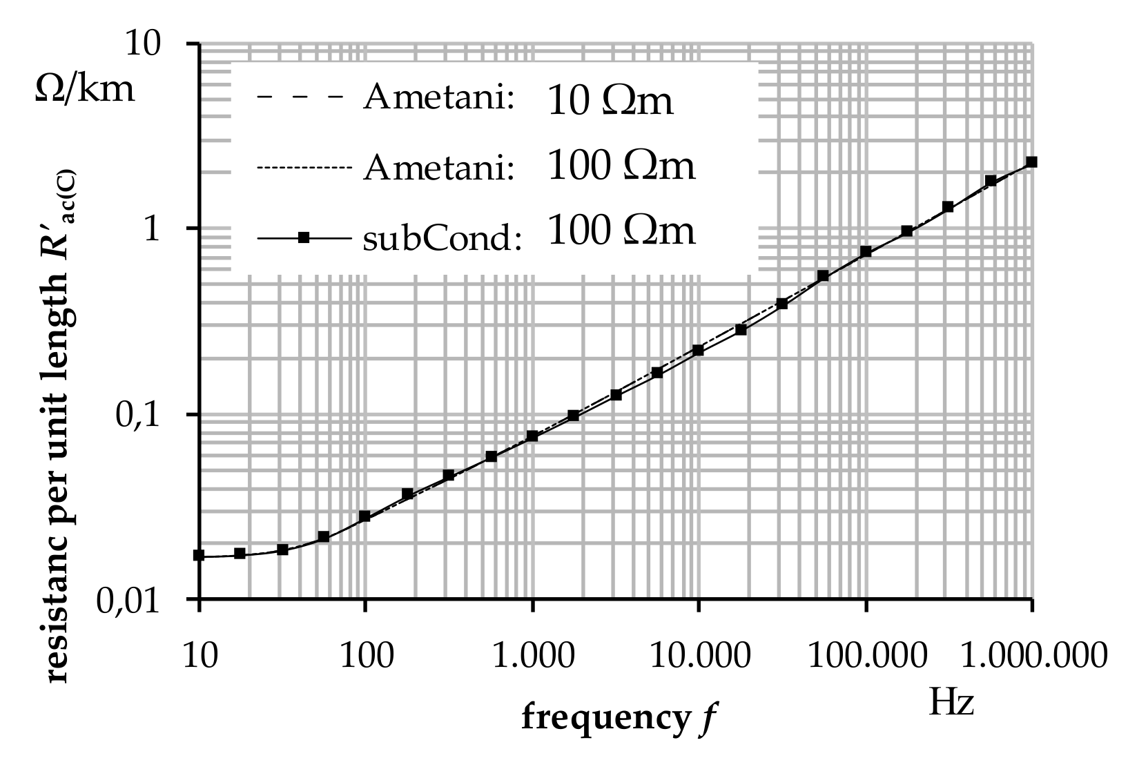
4. Validation of the Full Frequency-Dependent Cable Model

For the validation of the 3PPI model, a DC-Test on a three-phase cable with a length of $\ell \approx 2.5\mathrm{km}$ in trefoil formation has been used. The test is performed by charging the cable conductors up to 1 kV. After that, the charged conductors are connected to earth through the circuit breaker (s2) and the currents $i_{\mathrm{core}\left(\mathrm{A}\right)}$, $i_{\mathrm{core}\left(\mathrm{B}\right)}$, $i_{\mathrm{shield}\left(\mathrm{A}\right)}$ and $i_{\mathrm{shield}\left(\mathrm{B}\right)}$ at the sending end are measured. The test configuration is shown in Figure 18. The cable parameters are given in

Table 2. Parameters of 20-kV cable, NA2XS(FL)2Y.

Name	Unit	Value
Outer radius of the core $r_1$	$\mathrm{mm}$	$11.9$
Inner radius of the sheath $r_2$	$\mathrm{mm}$	$19.0$
Outer radius of the sheath $r_3$	$\mathrm{mm}$	$20.1$
Outer insulation radius $r_4$	$\mathrm{mm}$	$23.5$
Core resistivity ${\varrho }_{\mathrm{c}}$	$\mathsf{\Omega }\mathrm{m}$	$2.82\times {10}^{-8}$
Shield resistivity ${\varrho }_{\mathrm{s}}$	$\mathsf{\Omega }\mathrm{m}$	$1.70\times {10}^{-8}$
Inner insulation $tan\delta$		$4\times {10}^{-4}$
Outer insulation $tan\delta$		$4\times {10}^{-4}$
Inner insulation relative permittivity ${\epsilon }_{\mathrm{r}}$		$2.3$
Outer insulation relative permittivity ${\epsilon }_{\mathrm{r}}$		$2.4$
Relative permeability ${\mu }_{\mathrm{r}}$		$1.0$
Earth resistivity ${\rho }_{\mathrm{E}}$	$\mathsf{\Omega }\mathrm{m}$	150
Type of installation		Trefoil
Laying depth (system center)	$d_{\mathrm{d}}$	$1.2\mathrm{m}$
Length	ℓ	≈2.5 $\mathrm{km}$

.

The capacitances are calculated with Equations (19) and (20). The calculated frequency-dependent self resistance $R_{\mathrm{self}}^{\prime }$ and self inductance $L_{\mathrm{self}}^{\prime }$ are shown in Figure 19. The simulations with the 3PPI model have been executed with 75 PI sections. The order of approximation for ${\underline{\mathit{Z}}}_{\mathrm{m}\mathrm{fit}}^{\prime }$ and for ${\underline{\mathit{Y}}}_{\mathrm{L},\mathrm{m}\mathrm{fit}}^{\prime }$ is 8. The simulation time step is set to $\Delta t={10}^{-7}$ s. In this simulation, two facts should be replicated correctly: the wave travel time $\tau$, which is related to the imaginary term of $\underline{\gamma }$ and the attenuation, which is related to the real term of $\underline{\gamma }$. For the sake of clearness, Figure 20 shows only a comparison between the outcomes of 3PPI Model with the measured currents for the core and shield A. The comparison shows that the model results match very well with the measured data. This means that the wave travel time and attenuation are replicated correctly in the developed cable model which proves its validity. For example, in our case the simulated wave travel time is 14.8 $\mathsf{\mu }$s and the measured value is 14.5 $\mathsf{\mu }$s. The small deviation between the travel times (0.3 $\mathsf{\mu }$s) can also be minimized by increasing the number of PI sections. However, this will increase the calculation time.

In addition, it should be noted that a certain variation between simulation and measurement is always to be expected in general. This is mostly related to the lack of accurate information about some cable data, for example the thickness of inner and outer insulation screens and also their conductivity and permittivity. The inaccuracy in the cable data will affect the accuracy of the calculated longitudinal impedance ${\underline{\mathit{Z}}}^{\prime }$ and shunt admittance ${\underline{\mathit{Y}}}_{\mathrm{L}}^{\prime }$. This will be reflected in the simulation results of the cable model.

The required number of PI sections in the model depends on the expected frequencies in the transients, the cable length and the accepted calculation error. With the proposed model, calculation times of few seconds have been achieved.

5. Conclusions

In this paper, a full frequency-dependent cable model for calculations of transients was introduced. The frequency-dependent cable parameters are determined with an improved partial subconductor algorithm. The algorithm is able to handle a large number of conductors. Complete cable systems can be implemented including components like shields, armor, earth and other grounding conductors in parallel through the earth. If necessary, semiconducting layers can be realized in form of additional conductors. The skin and the proximity effect is considered in all conductors.

The improved partial subconductor method merely allows the calculation of the inductive coupling between conductor loops. The capacitive coupling is realized by other analytical methods. The frequency dependency of a XLPE insulation capacitance can be neglected for calculations in frequency ranges $f<5\mathrm{MHz}$.

The wave propagation cable model based on lumped parameters. A modal transformation technique was employed in the cable model to transform the cable system into decoupled single conductors. Every single conductor in the modal domain is represented through cascaded developed PI sections, where the frequency dependence of cable parameters is implemented through an RLC network in every PI section.

For an efficient computation time, the simulations in the time domain are executed using a recursive convolution technique. The number of PI sections in the full frequency-dependent cable model depends on the simulated cable length, the expected highest frequency in the investigated transient, and the accepted calculation error.

A comparison of the outcomes of proposed 3PPI model with measured data has shown a good match, which validates the approach used in developing this model.

A next important step is to compare the results of the developed full Frequency-dependent PI section cable model with other existing cable models, which is the goal of our next publication.

References

1. Ametani, A. A general formulation of impedance and admittance of cables. IEEE Trans. Power Appar. Syst. 1980, PAS-99, 902–909. [Google Scholar] [CrossRef]
2. Wedepohl, L.; Wilcox, D. Transient analysis of underground power transmission systems. Proc. IEE 1973, 120, 253–260. [Google Scholar]
3. Carson, J.R. Wave propagation in overhead wires with ground return. Bell Syst. Tech. J. 1926, 5, 539–554. [Google Scholar] [CrossRef]
4. Pollaczek, F. Über das Feld einer unendlich langen wechselstromdurchflossenen Einfachleitung. Elektr. Nachr. 1926, 3, 339–359. [Google Scholar]
5. Schelkunoff, A. The electromagnetic theory of coaxial transmission line and cylindrical shields. Bell Syst. Tech. J. 1934, 13, 532–579. [Google Scholar] [CrossRef]
6. Morched, A.; Gustavsen, B.; Manoocher, T. A universal model for accurate calculation of electromagnetic transients on overhead lines and underground cables. IEEE Trans. Power Deliv. 1999, 14, 1032–1038. [Google Scholar] [CrossRef]
7. Cgj, L.; Greeff, J.C.; Joubert, S.V. Modelling of telegraph equations in transmission lines. In Proceedings of the Buffelspoort TIME2008, Buffelspoort, South Africa, 22–26 September 2008. [Google Scholar]
8. Bekefi, G.; Barrett, H.A. Electromagnetic Vibrations, Waves, and Radiation; MIT Press: Cambridge, MA, USA, 1987. [Google Scholar]
9. Rusek, A.; Ganesan, S.; Aloi, N.D. A Friendly Approach to Transient Processes in Transmission Lines. In Proceedings of the 2011 ASEE North Central & Illinois-Indiana Section Conference, Mt. Pleasant, MI, USA, 1–2 April 2011. [Google Scholar]
10. Dommel, H.W. Electromagnetic Transients Program Manual (EMTP Theory Book); Bonneville Power Administration: Portland, OR, USA, 1986. [Google Scholar]
11. Snelson, J. Propagation of travelling waves on transmission lines-frequency dependent parameters. IEEE Transm. Power Appar. Syst. 1971, PAS-90, 2561–2567. [Google Scholar] [CrossRef]
12. Marti, J. Accurate modelling of frequency-dependent lines in electromagnetic transient simulations. IEEE Transm. Power Appar. Syst. 1982, PAS-101, 147–155. [Google Scholar] [CrossRef]
13. Marti, L. Simulation of transients in underground cables with frequency dependent modal transformation matrix. IEEE Transm. Power Appar. Syst. 1988, 3, 1099–1110. [Google Scholar] [CrossRef]
14. Noda, T.; Nagaoka, N.; Ametani, A. Phase Domain Modeling of Frequency-Dependent transmission Lines by Means of an ARMA Model. IEEE Trans. Power Deliv. 1996, 11, 401–411. [Google Scholar] [CrossRef]
15. Gustavsen, B.; Semlyen, A. Rational approximation of frequency domain responses by Vector Fitting. IEEE Trans. Power Deliv. 1995, 21, 1052–1061. [Google Scholar] [CrossRef]
16. Gustavsen, B.; Morched, A.; Manoocher, T. Improving the pole relocating properties of vector fitting. IEEE Trans. Power Deliv. 2006, 21, 1587–1592. [Google Scholar] [CrossRef]
17. Noda, T. Identification of a multiphase network equivalent for electromagnetic transient calculations using partitioned frequency response. IEEE Trans. Power Deliv. 2005, 20, 1134–1142. [Google Scholar] [CrossRef]
18. Noda, T. Application of Frequency-Partitioning Fitting to the Phase-Domain Frequency-Dependent Modeling of Overhead Transmission Lines. IEEE Trans. Power Deliv. 2015, 30, 174–183. [Google Scholar] [CrossRef]
19. Noda, T. Application of Frequency-Partitioning Fitting to the Phase-Domain Frequency-Dependent Modeling of Underground Cables. IEEE Trans. Power Deliv. 2016, 31, 1776–1777. [Google Scholar] [CrossRef]
20. Kocar, I.; Mahseredjian, J. Accurate Frequency Dependent Cable Model for Electromagnetic Transients. IEEE Trans. Power Deliv. 2016, 31, 1281–1288. [Google Scholar] [CrossRef]
21. Hoshmeh, A.; Malekian, K.; Schufft, W.; Schmidt, U. A single-phase cable model based on lumped-parameters for transient calculations in the time domain. In Proceedings of the 15th International Conference on Environment and Electrical Engineering, Rome, Italy, 10–13 June 2015; pp. 731–736. [Google Scholar]
22. Küpfmüller, K. Einführung in die Theoretische Elektrotechnik, 2nd ed.; Springer: Berlin/Heidelberg, Germany; New York, NY, USA, 1973. [Google Scholar]
23. Maxwell, I.C. A Treatise on Electricity and Magnetism, 4th ed.; Oxford University Press: London, UK, 2002; Volume 2. [Google Scholar]
24. Brüderlink, R. Induktivität und Kapazität der Starkstrom-Freileitung, 1st ed.; Verlag, G., Ed.; Braun: Karlsruhe, Germany, 1954. [Google Scholar]
25. Rees, F. Einfluss des Erdreichs auf das Elektromagnetische und Thermische Verhalten von Hochspannungs- Gleichstrom-Kabeln. Ph.D. Thesis, Technische Universität Darmstadt, Darmstadt, Germany, 1977. [Google Scholar]
26. Comellini, E.; Invernizzi, A.; Manzoni, G. A computer program for determining electrical resistance and reactance of any transmission line. IEEE Transm. Power Appar. Syst. 1973, PAS-92, 308–314. [Google Scholar] [CrossRef]
27. Dommel, H.W. Computation of cable impedances based of subdivision of conductors. IEEE Trans. Power Deliv. 1987, PWRD-2, 21–27. [Google Scholar]
28. Lucas, R.; Taluktar, S. Advances in finite elemente techniques for calculation cable resistances and inductances. IEEE Trans. Power Appar. Syst. 1978, PAS-9711, 875–883. [Google Scholar] [CrossRef]
29. Schmidt, U.; Shirvani, A.; Probst, R. An improved algorithm for determination of cable parameters based on frequency-dependent conductor segmentation. In Proceedings of the IEEE PES Transmission and Distribution Conference, Orlando, FL, USA, 7–10 May 2012; pp. 241–246. [Google Scholar]
30. Schmidt, U. Frequenzabhängige Parameter von Kabeln zur Berechnung von Ausgleichsvorgängen im Zeitbereich. Ph.D. Thesis, Chemnitz Technical University, Chemnitz, Germany, 2013. [Google Scholar]
31. Arnold, A.H.M. Proximity effect in solid and hollow round conductors. J. IEE 1941, 88, 349–359. [Google Scholar]
32. Brakelmann, H. Analyse der Stromdichteverteilungen von Mehrleiteranordnungen mit einem iterativen Teilleiterverfahren. ETZ Archiv 1989, 11, 369–377. [Google Scholar]
33. Ruedenberg, R. Die Ausbreitung der Erdstroeme in der Umgebung von Wechselstromleitungen. Zeitschrift für Angewandte Mathematik und Mechanik 1925, 5, 361–389. [Google Scholar] [CrossRef]
34. Dommel, H.W. Digital computer solution of electromagnetic transients in single- and multiphase networks. IEEE Trans. Power Appar. Syst. 1969, PAS-88, 388–399. [Google Scholar] [CrossRef]
35. Ametani, A.; Miyamoto, Y.; Nagaoka, N. Semiconducting layer impedance and its effect on cable wave-propagation and transient characteristics. IEEE Trans. Power Deliv. 2004, 19, 1523–1531. [Google Scholar] [CrossRef]
36. Liu, T. Dielectric Spectroskopy of Very Low Loss Model Power Cables. Ph.D. Thesis, University of Leicester, Leicester, UK, 2010. [Google Scholar]
37. Hadid, S.; Schmidt, U.; Schufft, W.; Rätzke, S. Frequenzabhängigkeit des Verlustfaktors tan δ an VPE-isolierten Kabeln. In Proceedings of the ETG-Fachtagung, Diagnostik Elektrischer Betriebsmittel, Fulda, Germany, 15–16 November 2012. [Google Scholar]
38. Wagenaars, P.; Wouters, P.; Wielen, P.; Steenis, E. Approximation of transmission line parameters of single-core and three-core XLPE cables. IEEE Trans. Dielectr. Electr. Insul. 2010, 17, 106–115. [Google Scholar] [CrossRef]
39. Gustavsen, B.; Sletbak, J.; Henriksen, T. Calculation of electromagnetic transients in transmission cables and lines taking frequency dependent effects accurately into account. IEEE Trans. Power Deliv. 1995, 10, 1076–1084. [Google Scholar] [CrossRef]
40. Steinbigler, H. Anfangsfeldstärken und Ausnutzungsfaktoren Rotationssymmetrischer Elektrodenanordnungen in Luft. Ph.D. Thesis, Technische Universität München, Munich, Germany, 1969. [Google Scholar]
41. Probst, R. Ermittlung der Kapazitäten des Drehstrom-Kabelsystems. Bachelor’s Thesis, Chemnitz Technical University, Chemnitz, Germany, 2011. [Google Scholar]
42. Marti, J. The Problem of Frequency Dependence in Transmission Line Modelling. Ph.D. Thesis, University of British Columbia, Vancouver, BC, Canada, 1981. [Google Scholar]
43. Chrysochos, A.I.; Papadopoulos, T.A.; Papagiannis, G.K. Robust Calculation of Frequency-Dependent Transmission-Line Transformation Matrices Using the Levenberg Marquardt Method. IEEE Trans. Power Deliv. 2014, 29, 1621–1629. [Google Scholar] [CrossRef]
44. Scott-Meyer, W. EMTP—Rule Book; Manual, Bonneviller Power Administration: Portland, OR, USA, 1982. [Google Scholar]
Figure 1. Equivalent configuration for the determination of the mutual inductance M between linear conductor loops.
Energies 10 01158 g001
Figure 2. Principal configuration for the determination of mean geometric distance g.
Energies 10 01158 g002
Figure 3. Equivalent circuit for determination of mutual inductance M m n with common return (hull cylinder).
Energies 10 01158 g003
Figure 4. Principle of conductor segmentation into subconductors.
Energies 10 01158 g004
Figure 5. Current density J C / J max ( C ) in a cylindrical conductor at different frequencies f.
Energies 10 01158 g005
Figure 6. Segmentation of a conductor into five skins.
Energies 10 01158 g006
Figure 7. The geometry of an arc segment.
Energies 10 01158 g007
Figure 8. Example for a segmentation of a conductor into three skins at frequency f = 50 Hz .
Energies 10 01158 g008
Figure 9. Current density J E / J max ( E ) in the earth at different frequencies f.
Energies 10 01158 g009
Figure 10. Segmentation of the earth into ten skins.
Energies 10 01158 g010
Figure 11. Structure of stranded rigid copper conductor.
Energies 10 01158 g011
Figure 12. One-skin segmentation of the inner semiconducting layer.
Energies 10 01158 g012
Figure 13. Resistance per unit length R ac C considering the semiconducting layer.
Energies 10 01158 g013
Figure 14. Configuration of a single core cable.
Energies 10 01158 g014
Figure 15. Representation of the frequency dependence of the cable longitudinal impedance.
Energies 10 01158 g015
Figure 16. PI section with the frequency dependence.
Energies 10 01158 g016
Figure 17. Principle of the three-phase cable model. VF: vector fitting algorithm.
Energies 10 01158 g017
Figure 18. Test configuration for the current measurements.
Energies 10 01158 g018
Figure 19. Simulated frequency-dependent self resistance R self and self inductance L self .
Energies 10 01158 g019
Figure 20. Comparison of simulated currents with measured data.
Energies 10 01158 g020