Nonlinear Adaptive Control of Heat Transfer Fluid Temperature in a Parabolic Trough Solar Power Plant


Abstract
:1. Introduction
2. Design
2.1. Adaptation
2.2. Prediction
- The controller output at time k, , must be the first value of a predicted controller output sequence in which all the increments in the interval are equal to zero. In the same interval, all the increments of the predicted disturbance sequence are assumed to be equal to zero.
- The predicted process output trajectory must be at time equal to a desired output value .
2.3. Initialization
- A generic, critically damped, second order linear model is chosen. A high gain of this model is desirable since it will avoid abrupt control actions during the first control instants.
- The controller is then started with the RBF network disabled and is updated at every control step according to Equation (6).
- After the linear model has somehow stabilized, it is set as and the regular operation described above in this section is started.
2.4. Sequence of Operations
- Obtain a measurement of the process output , along with a measurement of the variable vector .
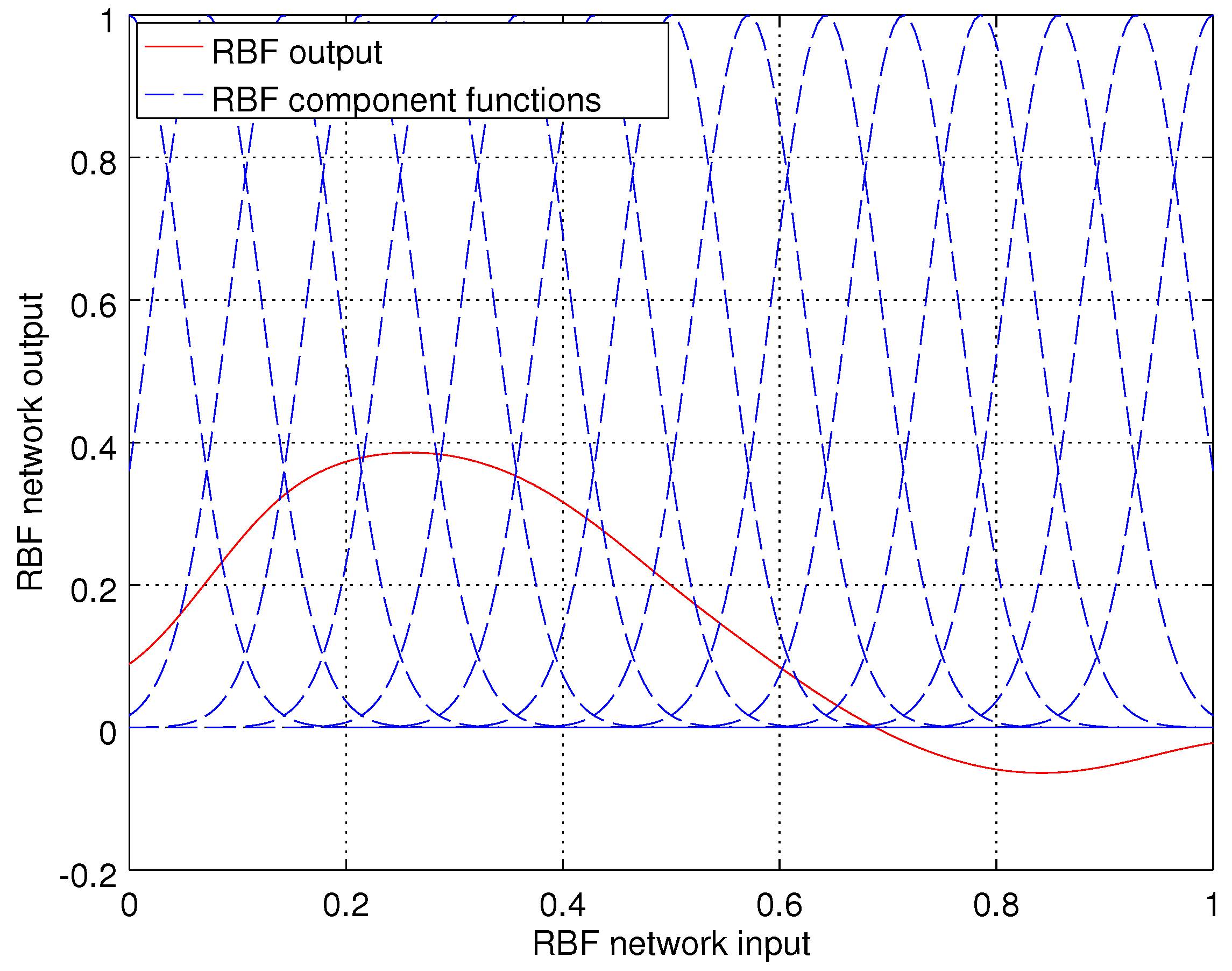
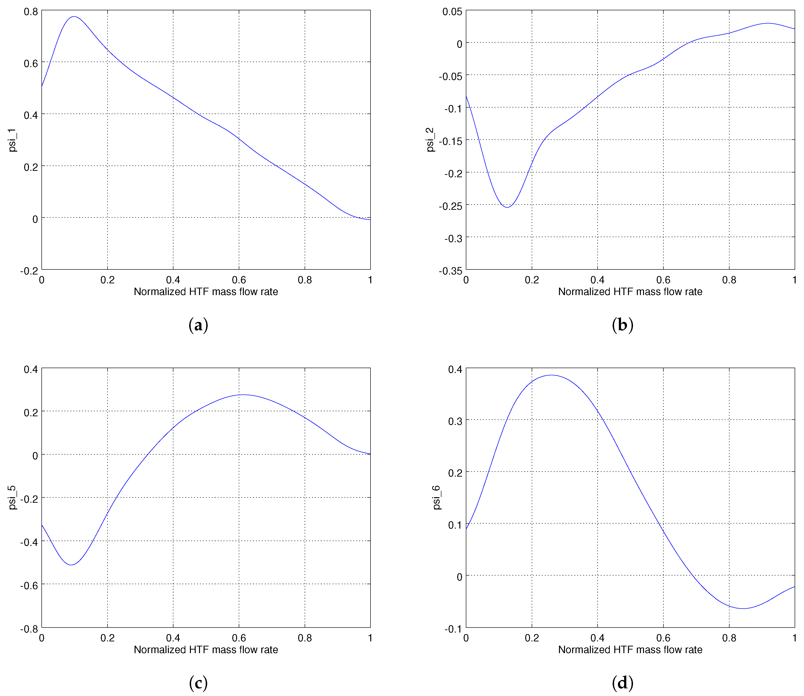
- Calculate the RBF network value at , , by using Equation (4).
- Obtain the expected process model linearization at , according to Equation (3).
- Obtain the new expected process model linearization at , according to Equation (3).
- Calculate the desired output process trajectory by using Equation (9).
- Calculate the control sequence as described in Section 2.2.
- Apply the first element of the calculated control sequence.
- Wait for the selected control period and repeat this sequence from the beginning.
3. Results and Discussion
3.1. Simulation
3.2. Control Scenario
3.3. Controller Configuration and Start-Up
- The controller sampling time has been set to 180 s.
- The variable under control, or process output, referred to as y in Equation (2) corresponds to the HTF final temperature and its set point has been set to 393 C.
- The control output, or process input, referred to as u in Equation (2) corresponds to the HTF pumps flow rate control loop set point in kg/s.
- The control action incremental limit has been set to 300 kg/s.
- The measurable disturbance referred to as d in Equation (2) corresponds to the measured DNI in W/m.
- The model size in Equation (2) has been set with the values , and .
- The horizon length referred to as in Equation (2) has been set to 7.
- The model parameters dependency set of variables referred to as in Equation (2) comprises only the circulating HTF mass flow rate as .
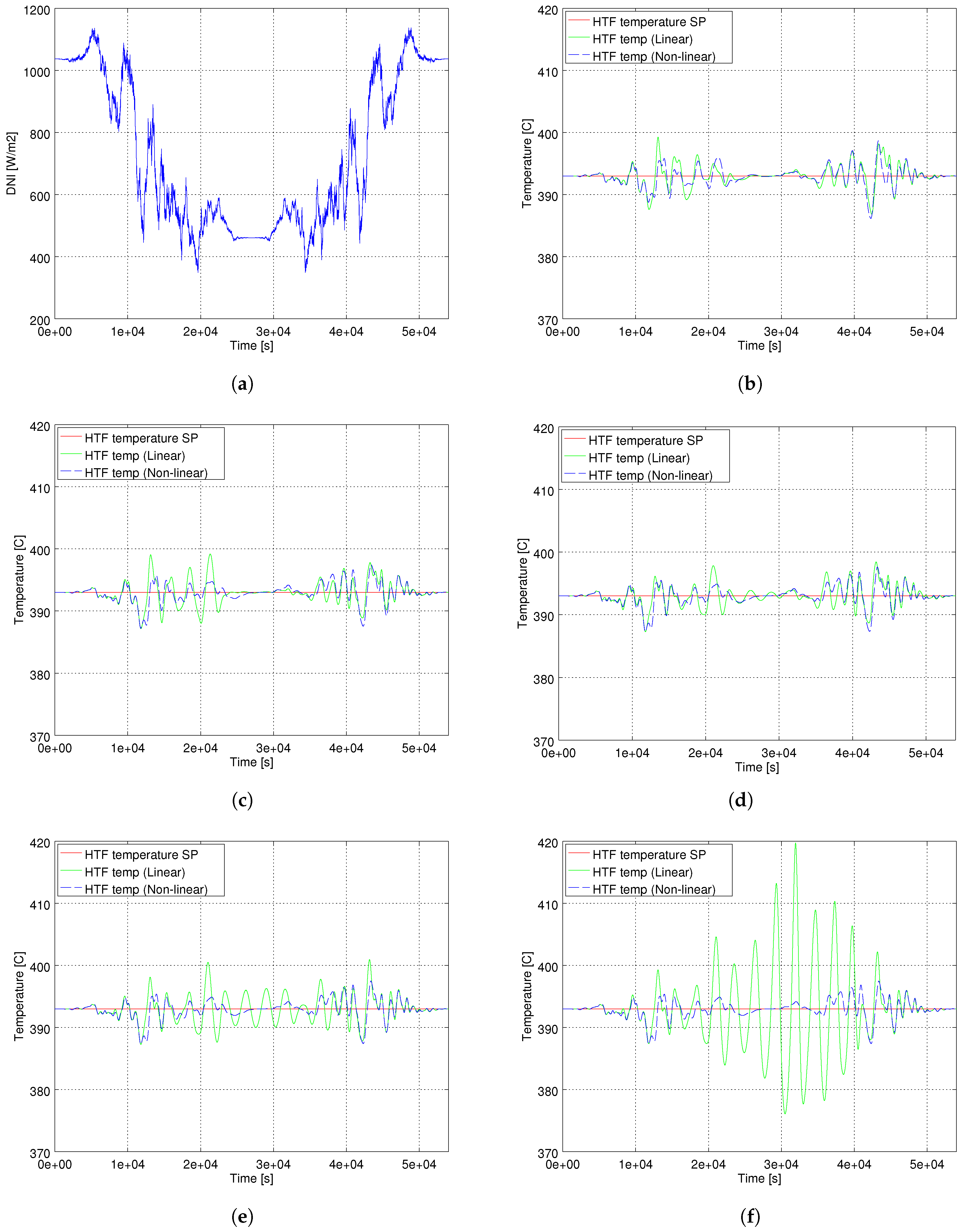
3.4. Performance Comparison
3.4.1. Regular Operation
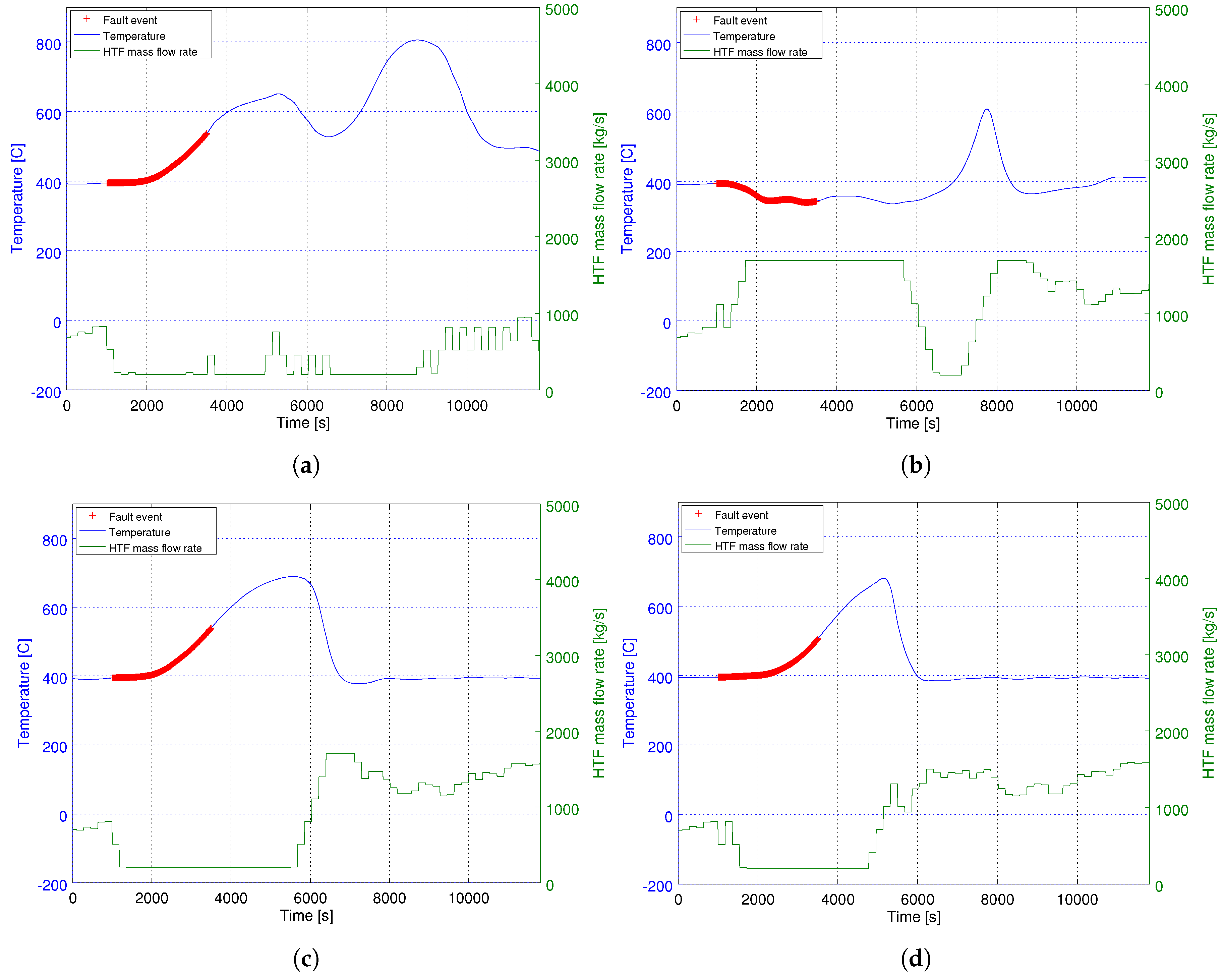
3.4.2. Fault Tolerance
3.5. Future Works
4. Conclusions
Author Contributions
Conflicts of Interest
References
- Rato, L.; Silva, R.; Lemos, J.M.; Coito, F.; Mosca, E.; Borreli, D.; Filatov, N.; Unbehauten, H. Adaptive predictive and switching control of a distributed collector solar field. In Proceedings of the CONTROLO—Portugese Conference on Automatic Control, Coimbra, Portugal, 9–11 September 1998. [Google Scholar]
- Leonessa, A.; Haddad, W.M.; Chellaboina, V.S. Nonlinear system stabilization via hierarchical switching control. IEEE Trans. Autom. Control 2001, 46, 17–28. [Google Scholar] [CrossRef]
- Pasamontes, M.; Álvarez, J.; Guzmán, J.; Lemos, J.; Berenguel, M. A switching control strategy applied to a solar collector field. Control Eng. Pract. 2011, 19, 135–145. [Google Scholar] [CrossRef]
- Zhang, Y.; Chai, T.; Wang, H.; Fu, J.; Zhang, L.; Wang, Y. An adaptive generalized predictive control method for nonlinear systems based on ANFIS and multiple models. IEEE Trans. Fuzzy Syst. 2010, 18, 1070–1083. [Google Scholar] [CrossRef]
- Kandare, G.; Nevado, A. Adaptive predictive expert control of dissolved oxygen concentration in a wastewater treatment plant. Water Sci. Technol. 2011, 64, 1130–1136. [Google Scholar] [CrossRef] [PubMed]
- Cirre, C.; Valenzuela, L.; Berenguel, M.; Camacho, E. Feedback linearization control for a distributed solar collector field. Control Eng. Pract. 2007, 15, 1533–1544. [Google Scholar] [CrossRef]
- Khoukhi, B.; Tadjine, M.; Boucherit, M. Nonlinear continuous-time generalized predictive control of solar power plant. Int. J. Simul. Multidiscip. Des. Optim. 2015, 6, A3. [Google Scholar] [CrossRef]
- Camacho, E.; Rubio, F.; Berenguel, M.; Valenzuela, L. A survey on control schemes for distributed solar collector fields. Part I: Modeling and basic control approaches. Sol. Energy 2007, 81, 1240–1251. [Google Scholar] [CrossRef]
- Camacho, E.; Rubio, F.; Berenguel, M.; Valenzuela, L. A survey on control schemes for distributed solar collector fields. Part II: Advanced control approaches. Sol. Energy 2007, 81, 1252–1272. [Google Scholar] [CrossRef]
- Barcia, L.A.; Peón, R.; Martínez-Esteban, J.A.; José-Prieto, M.A.; Martín-Ramos, J.A.; Cos Juez, F.J.; Nevado, A. Dynamic modeling of the solar field in parabolic trough solar power plants. Energies 2015, 8, 13361–13377. [Google Scholar] [CrossRef]
- Nevado, A.; Martín, I.; Mur, F. Design and application of a steam temperature optimizer in a combined cycle. Int. J. Adapt. Control Signal Process. 2012, 26, 919–931. [Google Scholar] [CrossRef]
- Nevado, A.; Requena, R.; Viúdez, D.; Plano, E. A new control strategy for IKN-type coolers. Control Eng. Pract. 2011, 19, 1066–1074. [Google Scholar] [CrossRef]
- Kandare, G.; Viúdez-Moreiras, D.; Hernández-del-Olmo, F. Adaptive control of the oxidation ditch reactors in a wastewater treatment plant. Int. J. Adapt. Control Signal Process. 2012, 26, 976–989. [Google Scholar] [CrossRef]
- Broomhead, D.S.; Lowe, D. Radial Basis Functions, Multi-Variable Functional Interpolation and Adaptive Networks; Royal Signals and Radar Establishment: Malvern, UK, 1988. [Google Scholar]
- Goodwin, G.C.; Sin, K.S. Adaptive Filtering Prediction and Control; Prentice-Hall: Upper Saddle River, NJ, USA, 1984. [Google Scholar]
- Martín-Sánchez, J.M.; Rodellar, J. Adaptive Predictive Control: From the Concepts to Plant Optimization; Prentice-Hall International: Upper Saddle River, NJ, USA, 1996. [Google Scholar]


| Variance | |||||
|---|---|---|---|---|---|
| Linear model | 2.911 | 3.506 | 2.748 | 4.944 | 40.751 |
| Nonlinear model | 2.407 | 2.361 | 2.355 | 2.338 | 2.336 |
© 2017 by the authors. Licensee MDPI, Basel, Switzerland. This article is an open access article distributed under the terms and conditions of the Creative Commons Attribution (CC BY) license (http://creativecommons.org/licenses/by/4.0/).
Share and Cite
Nevado Reviriego, A.; Hernández-del-Olmo, F.; Álvarez-Barcia, L. Nonlinear Adaptive Control of Heat Transfer Fluid Temperature in a Parabolic Trough Solar Power Plant. Energies 2017, 10, 1155. https://doi.org/10.3390/en10081155
Nevado Reviriego A, Hernández-del-Olmo F, Álvarez-Barcia L. Nonlinear Adaptive Control of Heat Transfer Fluid Temperature in a Parabolic Trough Solar Power Plant. Energies. 2017; 10(8):1155. https://doi.org/10.3390/en10081155
Chicago/Turabian StyleNevado Reviriego, Antonio, Félix Hernández-del-Olmo, and Lourdes Álvarez-Barcia. 2017. "Nonlinear Adaptive Control of Heat Transfer Fluid Temperature in a Parabolic Trough Solar Power Plant" Energies 10, no. 8: 1155. https://doi.org/10.3390/en10081155
APA StyleNevado Reviriego, A., Hernández-del-Olmo, F., & Álvarez-Barcia, L. (2017). Nonlinear Adaptive Control of Heat Transfer Fluid Temperature in a Parabolic Trough Solar Power Plant. Energies, 10(8), 1155. https://doi.org/10.3390/en10081155