Numerical Investigation for the Impact of Single Groove on the Stall Margin Improvement and the Unsteadiness of Tip Leakage Flow in a Counter-Rotating Axial Flow Compressor

Abstract

A low-speed counter-rotating axial flow compressor (CRAC) with single circumferential grooved casing treatment (CT) was investigated numerically. Both steady and time-accurate numerical calculations were performed to study the effects of the single grooved CTs over the rear rotor on the stability enhancement and the unsteadiness of tip leakage flow (TLF) in the CRAC. Parametric studies indicate that the best position of the single groove should be located near about 20% axial tip chord in terms of the stall margin improvement (SMI). The coincidence of the effective CT locations and the high fluctuating region on blade pressure surface in the smooth wall case shows that the unsteadiness of TLF plays an important role in the stall inception process. Frequency analysis for the static pressure signals near the blade tip shows that both the disappearance of the low frequency components and the suppression of unsteady TLF are beneficial to the SMI. Detailed observation of the flow structures illustrates that the action of the grooves on the different parts of TLF is responsible for the difference of SMI in the CTs. It is more effective to improve the flow stability by controlling the critical TLF released from near the mid-chord.

1. Introduction

Tip leakage flow (TLF) is well known as an important factor to impact the compressor performance, as measured in terms of pressure rise ability, efficiency and stability [1,2]. Up to now, much effort has been made to reveal the nature of TLF and researchers have made noteworthy progress on the potential relation between the stall inception and the unsteady phenomena in the tip region [3,4,5,6,7,8,9,10,11,12]. It has been found that the TLF could become unsteady at high loading operating conditions and the tip leakage vortex plays an important role in the stall inception process.

Both active flow control method (such as plasma actuation [13], fluidic actuators [14], and aspiration techniques [15]) and passive flow control method (such as blade tip modifications [16], blade tip winglet [17] and casing treatment) have been carried out by a large number of researchers to expand stall margin and improve the compressor performance by controlling the impact of the TLF. As a passive flow control method, casing treatment (CT) has been proven to have a beneficial effect on enlarging the stable operating range of compressors. To obtain an adequate CT configuration for real compressors, a large amount of work has been conducted on the effects of CTs on the unsteady flow structures in the tip region. Past research showed that the interaction between the unsteadiness of the TLF and the CTs is of great importance for the compressor performance. Zhao and Lu [18] conducted an investigation of the circumferential grooves on the TLF and stall margin improvement (SMI) numerically. It was found that the delay of the happening of TLF unsteadiness is responsible for the extension of the compressor stall margin. Hwang [19] investigated the effect of CT on the unsteadiness of TLF in a low-speed axial compressor and the result showed that the unsteady strength of the TLF was alleviated by the CT. Du et al. [20] numerically studied the effect of single grooves at different axial location on the self-induced unsteadiness of TLF in a low-speed axial compressor. It demonstrated that the single groove location affected not only the oscillating strength but also the frequency of the TLF. At the mass flow corresponding to the near-stall condition of the smooth wall (SW) case, the more the fluctuation amplitude of TLF was intensified, the higher the SMI obtained with the groove. The frequency component became more complicated as the single groove was moved from the blade leading edge to the trailing edge. It was also found that the stall pattern of the original SW compressor stage can be changed by the application of the CTs [21,22,23,24]. Additionally, the stall precursor-suppressed CT designed by Sun et al. indicates that the unsteady CT can delay the nonlinear development of stall process by suppressing the propagation of inception wave [25,26,27]. Although the physical mechanism of CT for SMI is still not fully understood, all the results above indicate that the SMI of compressors is closely related to the impact of the CT grooves on the TLF unsteadiness.

Recently, the counter-rotating axial flow compressor (CRAC) attracts great intention because it enables the reduction of the engine weight by removing of the stator blade row between the adjacent rotors [28,29]. Endeavors to gain further insights into the flow physics in CRAC have been conducted on the important factors, including axial spacing between two rotors, unsteady effects, inlet distortion, etc. [30,31,32,33,34,35,36,37,38]. Compared with a conventional compressor stage, it was found that there are many new characteristics and unique flow phenomena in CRAC. For example, it has been found that a contra-stage produces a stall free characteristic when the second rotor is contra-rotated at a speed faster than the first rotor. A higher rotational speed of the second rotor has a beneficial effect on the overall performance due to the strong suction generated by higher rotational speed of the second rotor with circumferential inflow distortion. Additionally, the flow fields in the second rotor are more complicated and challenging due to its higher aerodynamic loading than the front rotor. The changes of the compressor performance and unsteady phenomena inside are more sensitive to the tip gap size variation of the second rotor.

However, there has been limited information so far in the open literature about the detailed study on the CTs in CRAC except the work conducted by Pundhir et al. [39], in which three types of CTs, namely axial slots, axial skewed slots and circumferential grooves, were investigated experimentally. It was found that the circumferential grooves type CT was the most suitable. Moreover, there has not been any investigation about the interaction between the CTs and the unsteadiness of TLF in CRAC. Therefore, it seems worthwhile to make a study on the impact of single grooved CT at different locations on the unsteadiness of the TLF and its potential effects on SMI in the CRAC.

In this paper, we will mainly focus on how the axial location of a single casing groove affects the stability enhancement and the unsteadiness of TLF in the CRAC. This paper is organized as follows: after the introduction of the investigated CRAC and the grooved CTs design in Section 2, the numerical method and its validation are shown in Section 3. Thereafter, the impacts of the CTs on the unsteady flow behaviors and the corresponding mechanisms related to the SMI are presented in Section 4. Finally, a short conclusion is shown in Section 5.

2. Compressor Geometry and CT Design

The test case considered for this study is a low-speed two-stage CRAC in Northwestern Polytechnical University (NWPU). Figure 1 shows the pictures and a cross-sectional diagram of the CRAC. The compressor consists of four blade rows, i.e., inlet guide vane (IGV) with 22 blades, a clockwise rotating rotor (R1), an anti-clockwise rotating rotor (R2), and an outlet guide vane (OGV) with 32 blades. Two AC motors are used to drive the two rotors, respectively. The mass flow rate and total pressure ratio of the CRAC at design point are about 6.4 kg/s and 1.22, respectively.

Table 1. Other main design parameters of the two rotors.

Design Parameter	R1	R2
Blade number	19	20
Tip clearance (mm)	0.5	0.5
Hub-tip ratio	0.485	0.641
Rotational speed (rpm)	8000	−8000
Tip blade chord (m)	0.0832	0.0769
Tip speed (m/s)	167.6	167.6

presents the other main design parameters of the CRAC.

Previous research on this compressor has indicated that the flow fields in the tip region of R2 are responsible for the spike-type flow instability of the CRAC [35,37,38]. Therefore, different circumferential single grooves over the blade tip of R2 were numerically investigated in the current paper. The schematic of the circumferential grooved CTs and the enlarged view of grid near the groove are shown in Figure 2. The location of single groove is defined as the axial distance of the groove leading edge from the blade leading edge normalized by the axial chord of blade tip (Ca). For example, a circumferential groove with its leading edge positioned at 20% tip axial chord length downstream of the blade leading edge is named G2.

Considering the design parameters of grooves in past research and the mechanical integrity of compressor with CT, both the axial depth and width of the grooves are 2 mm (about 5.8% Ca) in the current paper, giving an aspect ratio (AR) of 1. Generally, the CTs with the deeper and wider grooves can generate more SMI within a certain range of groove size, but they often cause a larger efficiency loss in the meanwhile. It is well known that the best location and size of the grooves can only be obtained by conducting a large number of numerical simulations or experiments. Therefore, it should be mentioned here that the influence of groove size is not the focus of the current paper and the impact of the parameters of both width and depth on the SMI will be investigated in near future work.

An enlarged view of the mesh near the groove is also shown in Figure 2. In this paper, the grid of the casing grooves was generated in H topology by IGG [40] from NUMECA (Numerical mechanics application) International. This mesh has 0.39 × 10⁵ nodes with 21 axial, 21 radial, and 89 tangential points. The groove mesh was connected with the main blade passage by the full non-matching connecting technology [40], a technique that allows arbitrarily connecting grid blocks of different grid topologies to each other without significant numerical interpolation losses.

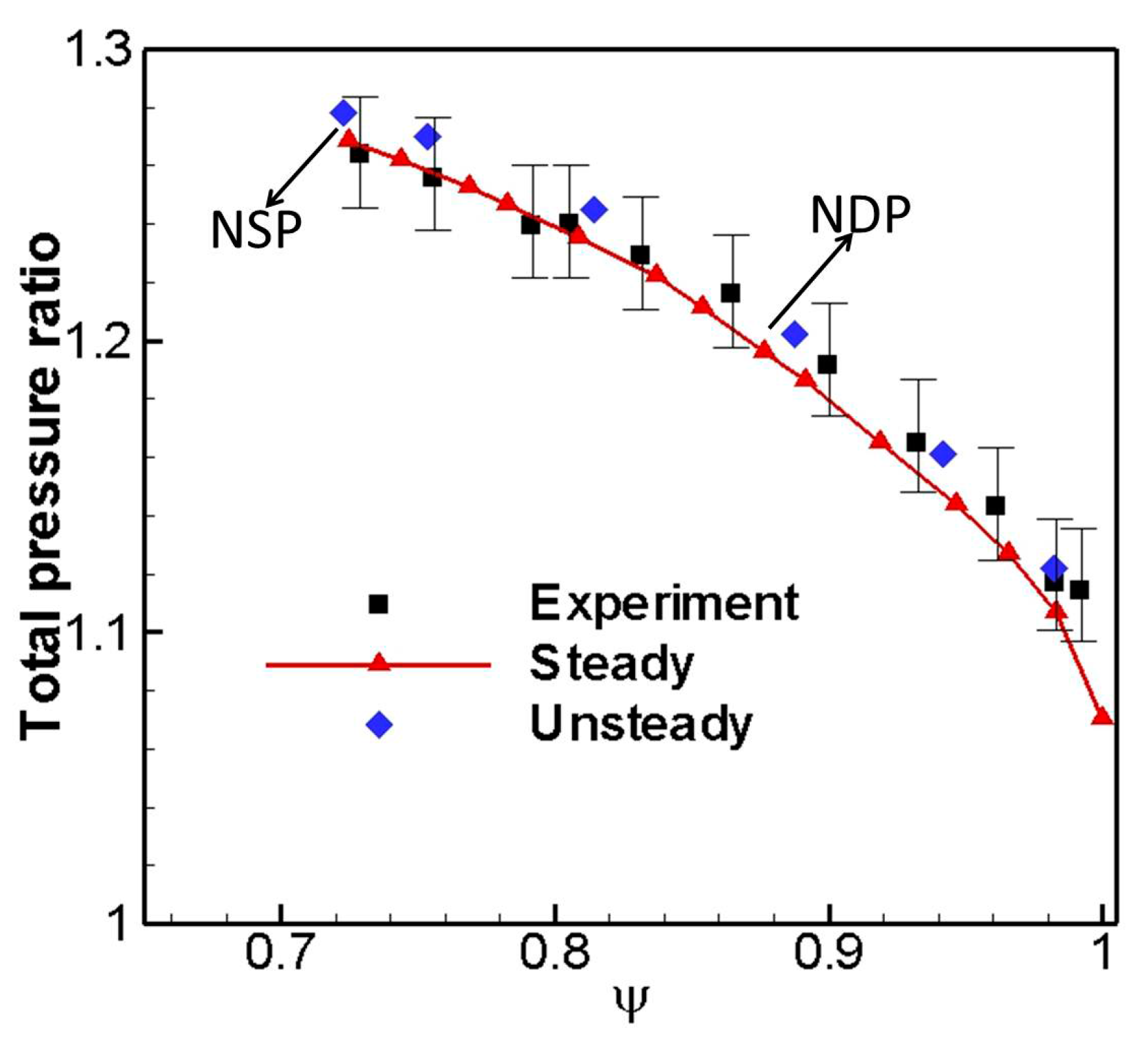
3. Numerical Method and Validation

A commercial solver package, FINE/TURBO [41] from NUMECA International, was used for the computations in the present work. Single-passage simulations were performed by solving steady and unsteady compressible three-dimensional (3D) RANS (Reynolds Averaged Navier-Stokes) equations on structured multi-block grid. The equations were discretized in space using a cell-centered finite volume scheme. For steady simulations, the explicit fourth-order Runge-Kutta scheme was adopted for the time discretization. Time-accurate unsteady computations were based on the implicit dual-time stepping technique and each instantaneous flow solution was considered as a pseudo-steady problem in which an explicit fourth-order Runge-Kutta scheme with local time step was adopted. The unsteady calculations used the domain scaling method [41] to deal with the interface of the two rotors. It requires each blade row in the mesh to cover the same circumferential distance. Therefore, the blade number of R1 was changed from 19 to 20 with the blade solidity unchanged by changing the blade chord length. The displacement of one rotor pitch was discretized with 80 physical time steps and 50 pseudo time iterations were performed for each physical time step.

One equation turbulence model of Spalart-Allmaras (S-A) [42] was employed to estimate the eddy viscosity. No-slip and no-heat transfer conditions were imposed at the solid boundaries. Total pressure, total temperature and flow angles were given uniformly at the inlet boundary. Radial equilibrium static pressure boundary condition was adopted on the outlet plane in the steady simulations. For the time-accurate unsteady computations, the identical mass flow rate was specified at the outlet boundary condition in two typical grooved CTs to keep the same incoming flow condition. In order to predict the numerical stall margin of the CRAC accurately, the back pressure dichotomy method was used in the steady computations [43]. The static pressure and its step change were both renewed gradually as the operating condition approaching the stall point. The stability limit was determined by the first divergence point in the numerical simulation process as the mass flow coefficient was reduced.

The mesh for the computations was generated by AUTOGRID5 [44]. O4H topology was chosen to model the main flow passage and butterfly topology was adopted to model the real tip gap in the rotors. The investigation of grid independence for the CRAC has been performed by Wang [36] in which six mesh schemes of the compressor with 1.19 × 10⁶, 1.38 × 10⁶, 1.51 × 10⁶, 1.78 × 10⁶, 2.03 × 10⁶, and 2.42 × 10⁶ grid cells were studied to exclude the effect of grid size. It was found that the obtained total pressure ratio and isentropic efficiency of the CRAC kept almost unchanged if the grid number exceeds about 2.03 × 10⁶. Therefore, a total grid number of about 2.6 × 10⁶ was adopted for the computations of the four blade rows in the current paper. Compared with the passage grid near the blade tip, a much finer mesh is used for the grooves to ensure that the complicated flow details near the grooves can be captured precisely. The grid density was increased near the solid boundaries to keep y+ ≤ 3 at the walls with the minimum grid spacing of 5 × 10⁻⁶ m on the solid wall, which satisfies the requirement of the S-A turbulence model, i.e., the value of y+ is no more than 10 [41]. The computational mesh in the two rotors together with the enlarged views of the grid near the tip leading edge and trailing edge are shown in Figure 3.

To validate the numerical method used in the present work, the comparison between the calculated and experimental total pressure ratio performance curve at design speed is shown in Figure 4. The numerical results were obtained from a number of steady and unsteady computations. Two pressure rakes was located upstream of the IGV and downstream of the OGV to get the inlet and outlet total pressure in the experiment. The radial distribution of the total pressure was mass averaged across the annulus. Unlike the steady computations and experiment, the unsteady numerical simulations were conducted only for the two rotors. Both the mass-averaged inlet and outlet total pressure are obtained at the same location of the experiment in the steady and unsteady simulations. One can see that the overall performance curves between the steady numerical results and experiments agree well for the most part, especially at the near-stall points. The results predicted by unsteady numerical simulations are slightly higher than the experiments. Figure 5 shows the predicted absolute total pressure contours on the 90% blade span of IGV and OGV at the near-stall point of the steady simulation. It can be seen that the total pressure loss in the OGV caused by the flow separation on the blade suction side is more obvious than that in the IGV which is mainly due to the development of boundary layer. Therefore, the discrepancy is probably because the total pressure losses in the IGV and OGV are not included in the unsteady simulations, unlike the experimental results. However, the error analysis of the performance curves and the agreement between experiment and numerical simulations give us confidence in the use of the numerical method to draw conclusions about the flow features in the compressor.

4. Results and Discussion

4.1. Effects of CTs on the SMI

Parametric studies in terms of SMI were performed first with respect to the axial location of the single groove by the steady simulations. Ten circumferential single grooves were studied in the current paper. Figure 6 shows the total pressure characteristics derived from the simulations with and without CT. In order to present the results clearly, only six typical cases are plotted. It should be mentioned that the computational domain was simplified by removing the IGV and OGV to save the computation cost in these simulations. Therefore, the absolute values of the total pressure ratio in the SW case shown as Figure 6 are slightly higher than that in Figure 4. From Figure 6, it can be seen that the stall point flow coefficient is reduced obviously for the schemes of G1, G2 and G3 compared with the SW case, especially G2 and G3. Additionally, no distinctive change of the total pressure ratio can be observed until the operating condition close to the stall point.

In the present work, the stability enhancement performances of CTs are evaluated by the change of stall margin (ΔSM) which is defined as the equation below:

$$\Delta \mathrm{SM}={[\frac{{\pi }_{\mathrm{stall}}{m}_{\mathrm{design}}}{{\pi }_{\mathrm{design}}{m}_{\mathrm{stall}}}-1]}_{\mathrm{CT}}-{[\frac{{\pi }_{\mathrm{stall}}{m}_{\mathrm{design}}}{{\pi }_{\mathrm{design}}{m}_{\mathrm{stall}}}-1]}_{\mathrm{SW}}$$

(1)

The ΔSM trend versus groove location is shown in Figure 7. One can see that the location interval for good SMI is fairly wide, i.e., from the blade leading edge to 40% Ca, while the effect of CTs after 40% Ca on the ΔSM seems insignificant. The stall margin is improved by about 4.0% for the G2 location. Therefore, the best location for the single groove in the CRAC should be at about 20% Ca downstream of the blade leading edge, where there is a broad and safe peak in the improvement of stall margin. It is well known that the unsteady TLF plays an important role in the process of stall inception. To obtain the effects of single groove location on the unsteadiness of the TLF and its possible link to the SMI, the inside fluctuations and unsteady behaviors near the blade tip will be analyzed in the following section.

4.2. The Impact of CTs on the Inside Unsteady Fluctuations

Two typical groove locations of G2 and G3 will be used then to study the influence of CTs on the unsteady flow phenomena at near-stall condition and the corresponding mechanisms of the SMI. The analysis was conducted at the same normalized mass flow rate of about 0.68. The variation of unsteady fluctuations in R1 is not reported here because the effect of the CTs on the flow fields in R1 is insignificant.

The leading edge spillage of the interface (between the TLF and incoming main flow) and the initiation of backflow at trailing edge plane are two conditions necessary for the occurrence of spike-type disturbances and the stall limit will only occur when the latter event comes about [45]. Therefore, the delay of the interface spillage is often used to evaluate the stability enhancement. Time-averaged relative total pressure coefficient contours and surface streamlines on the plane of the blade tip are shown in Figure 8. The interface is indicated as a green dash-dotted line and a black circle is used to indicate the relative position between interface and the pressure side of the neighboring blade.

In Figure 8, one can see that the interface of the SW case has already been pushed out of the blade leading edge plane and the leading edge spillage of the TLF to the adjacent passage happens. For the two CTs, although there is still the phenomenon of leading edge spillage, the interfaces are pushed downstream to different extents. Additionally, we can observe that the intensity of the TLF is decreased compared with the SW case from the red line with arrow, especially in G2.

Figure 9 shows the time-averaged and pitch-averaged absolute vorticity contours on the meridional plane for the SW case and two CTs. The vertical and horizontal red dash-dotted lines represent the left and lower boundaries of the high absolute vorticity region, respectively, in the SW case. The absolute vorticity is defined as below:

$${\xi }_n=\frac{\left|\xi \right|}{2\omega }$$

(2)

where $\left|\xi \right|$ and $\omega$ denote the magnitude of vortex vector and angular velocity of the rotor, respectively.

Generally, the value and range of the absolute vorticity can be used to evaluate the intensity of TLF. Compared with the SW case, the high absolute vorticity area is decreased remarkably in the two CTs, especially in G2. The influence range of TLF is reduced in both spanwise and streamwise direction, which indicates the reduction of TLF intensity due to the impacts of the CTs. Therefore, the tip flow fields in R2 are improved by the CTs.

The static pressure coefficient distributions on blade surfaces of 99% span at four different time steps within one numerical period are shown in Figure 10. For the SW case, one can observe that there are two high fluctuating regions on the blade surfaces near the tip. One is located on the pressure surface ranging from blade leading edge to about 45% Ca and the other one is on the blade suction surface ranging from about 60% Ca to the blade trailing edge. From the following analysis, the pressure fluctuations are mainly due to the impacts of the unsteady TLF and double leakage flow.

In Figure 10b,c, it can be seen that the pressure oscillating strength on the pressure surface is reduced in the two grooved CTs and G2 is the most effective scheme in suppressing the oscillation on the blade pressure side. The pressure fluctuations on the suction surface near the blade trailing edge also decrease due to the change of the tip flow fields, especially in G3. The locations of the two CTs plotted in Figure 10a also show that the G2 groove is just at the position of the peak fluctuation. From the analysis above, Figure 7 has shown that G2 is the best scheme to improve the flow stability and the grooved CT is effective only when its location is within the space between the blade leading edge and about 40% Ca, which is almost the same as the range of the high fluctuating region on the blade pressure surface. Therefore, we can conclude that the unsteadiness of TLF plays an important role in the stall inception process and there is a close link between the effectiveness of the CTs and the suppression of the unsteady TLF, which is consistent with the conclusion by Tong et al. [46]. He has found that spike was initiated at the circumferential location with the strongest unsteadiness.

To clearly view the location of the unsteadiness within the blade passage of R2, the contours of the standard deviation (STD) of static pressure distribution on the blade surfaces for the SW case and two CTs are shown in Figure 11. The value of static pressure STD can be used to indicate the distribution of pressure oscillating strength [9]. The STD of static pressure is defined as below:

$$\sigma =\sqrt{\frac{1}{N}{\displaystyle {\sum }_{i=1}^N{(P_i-\overline{P})}^2}}$$

(3)

where $P$ and $\overline{P}$ denote the local static pressure and time-average static pressure, respectively; i represents the time index of different time instant; and N represents the total number of time steps within one numerical period.

From the STD contours of static pressure in the SW case shown as Figure 11, one can see that the overall oscillation on the pressure surface is much stronger than that on the suction side, especially in the tip region. Firstly, a high static pressure STD region indicated by black dashed rectangle is concentrated on the blade leading edge for both surfaces due to the impingement of the incoming defective flows (i.e., wakes and TLF) from upstream or the local leading edge spillage of TLF. Additionally, there is another high static pressure STD zone on the pressure surface denoted by A in the tip region near blade leading edge, which corresponds to the location where the TLF or double leakage flow impinge on the adjacent blade pressure side most often.

In the cases with grooved CT, there are significant changes of the high static pressure STD zone A on the pressure surface in the two CTs compared with the SW case. For G2 grooved CT, the oscillating strength is decreased significantly and the high static pressure STD zone A is split into two parts, which is consistent with the results in Figure 10b, i.e., the peak unsteady fluctuation is suppressed by the groove of G2. The front part merges with the high static pressure STD region near the blade leading edge together and the rear part is shifted further downstream. In the grooved CT of G3, the fluctuating intensity of zone A is also reduced remarkably without obvious variation of its location, which indicates that the pressure oscillating strength of the TLF or double leakage flow is attenuated due to the impact of groove.

The oscillating frequency is another main characteristic of the unsteady TLF and the Fast Fourier transformation (FFT) results of the instantaneous signals are often used to observe the flow characteristics. In the current paper, the FFT is carried out for the static pressure signals of the monitoring points and the frequency characteristics are presented in the rotor relative frame. The FFT results for five numerical probes in the SW case and two CTs are shown in Figure 12. The five numerical monitors are positioned at the pressure side of 99.5% blade span along the tip chord, i.e., 1% Ca, 10% Ca, 30% Ca, 50% Ca and 80% Ca, respectively. One can see that the overall amplitude distribution of the unsteady static pressure in the SW case and CTs is consistent with the static pressure STD contours shown in Figure 11, i.e., the high amplitude of the static pressure signals is mainly located near the blade leading edge. It should be mentioned that there is a common dominating frequency of 1.0 blade passing frequency (BPF) in the SW case and two CTs. In light of the same blade number for both rotors in the unsteady simulations, the fluctuation frequency of 1.0 BPF is identical to the sweep frequency of the two rotors.

Apart from the inherent fluctuation frequency of 1.0 BPF, there exist three other fluctuation frequency components of 0.74 BPF, 0.31 BPF and 0.47 BPF in the SW case. According to the previous study of the unsteady flow behaviors in R2, the frequency of 0.74 BPF is mainly due to the self-induced unsteadiness of TLF near the blade tip [37]. For the two CTs, two main findings can be seen in Figure 12b,c. Firstly, the two lower fluctuation frequency components of 0.31 BPF and 0.47 BPF both disappear due to the impact of the CT grooves. It has been found that the occurrence of the low dominating frequency components is linked to the rotating instabilities [47,48]. Therefore, the vanishing of the low frequency components may probably contribute to the delay of stall inception and the SMI. Secondly, the frequency component related to the unsteadiness of TLF is changed from 0.74 BPF to 0.82 BPF in G2, while the G3 groove has no influence on the oscillating frequency of the unsteady TLF. Additionally, the amplitudes of the frequency component related to the self-induced unsteadiness of TLF are both decreased in the two CTs, which corresponds to the suppression of the unsteady TLF by the CT grooves as shown in Figure 10 and Figure 11. By comparing the common flow features of the two CTs, it can be inferred that both the vanishing of the low frequency components and the suppression of the TLF unsteadiness are beneficial to the SMI.

The STD static pressure contours on the middle plane of the grooves perpendicular to the axial direction in the two CTs are shown in Figure 13. Actually, the reason of the SMI generation is just due to the interaction between the grooves and TLF. The studies conducted by Shabbir and Adamczyk [49] and Chen et al. [50] implied that a groove located near the blade leading edge was more effective than the groove at the other tip chord range due to the stronger interaction of the groove near the leading edge with the TLF. From Figure 13, one can observe that the fluctuating strength in G3 is stronger than that in G2, while it has been found that G2 is more effective in improving the flow stability from the Figure 7. Therefore, the intensity of the interaction between the CT groove and the TLF is not the only decisive factor to impact the result of SMI. It seems that there exists a critical chord interval of TLF and the CT is more effective when its groove acts on the critical portion of TLF.

It has been found that the TLF along the chord can be divided into different parts and each part plays a different role on the stall inception mechanism in the tip region [9]. Generally, the TLF over the front portion governs the initial position of interface near the suction surface, while the rear portion of TLF interacts with the incoming flow near the pressure side of the neighboring blade and shifts the interface upstream, which may lead to the leading edge spillage of TLF. In the current paper, the most important two portion of TLF will be considered in the following analysis. The first portion of TLF called main TLF is released from blade leading edge to about 30% blade chord and the second portion of TLF called critical TLF is released from about 30% to 60% blade chord.

The time-averaged 3D flow streamlines released from mid-gap from leading edge to 60% blade chord colored with relative Mach number are presented in Figure 14. The typical 3D flow streamlines from mid-gap are used here to illustrate the impact of the CTs. For the SW case, one can observe that the critical TLF from near the mid-chord (denoted by red dashed line) arrives at the pressure side near the leading edge of the adjacent blade. Then the phenomena of local leading edge spillage and double leakage happen. The low energy fluid region (marked by black ellipse) at the blade leading edge near the pressure side is mainly caused by the critical TLF, which is often linked with the stall inception indicator (leading edge blockage near the pressure side) in past studies. The main TLF released from near the blade leading edge (denoted by black dashed line) mainly flows out of the passage directly and it only determines the initial location and direction of the interface.

For the CTs of G2 and G3, the extent of both the double leakage phenomenon and leading edge spillage near the blade leading edge (marked by black rectangle) is decreased obviously, especially in G2. According to the change of the low energy fluid region, it is also found that both the CTs can improve the tip flow fields significantly.

To obtain a deep insight into the effect of CTs on the flow fields, the changes of time-averaged main and critical TLF structures are shown in Figure 15 respectively. In Figure 15a, one can see that the main TLF in both the CTs becomes closer to the pressure side of the adjacent blade and concentrated in a smaller region. Additionally, the phenomena of both the double leakage and leading edge spillage near the blade leading edge are aggravated resulting from the main TLF in the two CTs. When considering the critical TLF, it is found that both the CTs of G2 and G3 share the same flow change behavior compared with the SW case. A part of critical TLF is redirected downstream and flows out of the passage directly due to the effect of casing grooves. Consequently, both the phenomena of leading edge spillage and double leakage near the blade leading edge are receded significantly, especially in G2. In view of the common flow characteristics in G2 and G3, we can conclude that it is more effective to improve the flow stability by controlling the critical TLF and the improvement of the main TLF is not necessary to achieve the effectiveness of SMI.

Figure 16 presents the STD static pressure contours at 99% blade span of R2 in the SW case and the two CTs of G2 and G3. Compared with the SW case, the high pressure oscillation on the pressure side marked by the red dashed oval in G2 is shifted more downstream and with the fluctuating intensity reduced obviously, which is probably due to the reason that the critical TLF is pushed more downstream and it becomes much further away from the pressure side of adjacent blade shown as Figure 15. Additionally, the high fluctuation region near the blade leading edge indicated by black dash-dotted rectangle is also decreased due to the improvement of the critical TLF in G2. For the CT at G3, the high oscillating zone near the blade leading edge indicated by black dash-dotted rectangle is reduced obviously and the pressure fluctuation on the pressure surface marked by red dashed oval is also reduced slightly due to the improvement of the critical TLF.

5. Conclusions

In the current paper, the impacts of single grooved CT at different axial locations on the SMI, the unsteadiness of TLF and the potential link of the effects to the SMI are investigated numerically in the rear rotor of a low-speed CRAC. Two typical effective CTs (G2 and G3) are used to conduct the unsteady analysis. The findings are summarized in detail as follows.

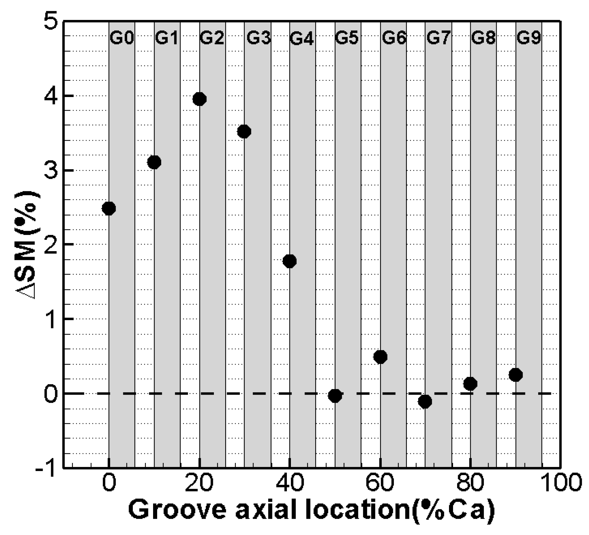
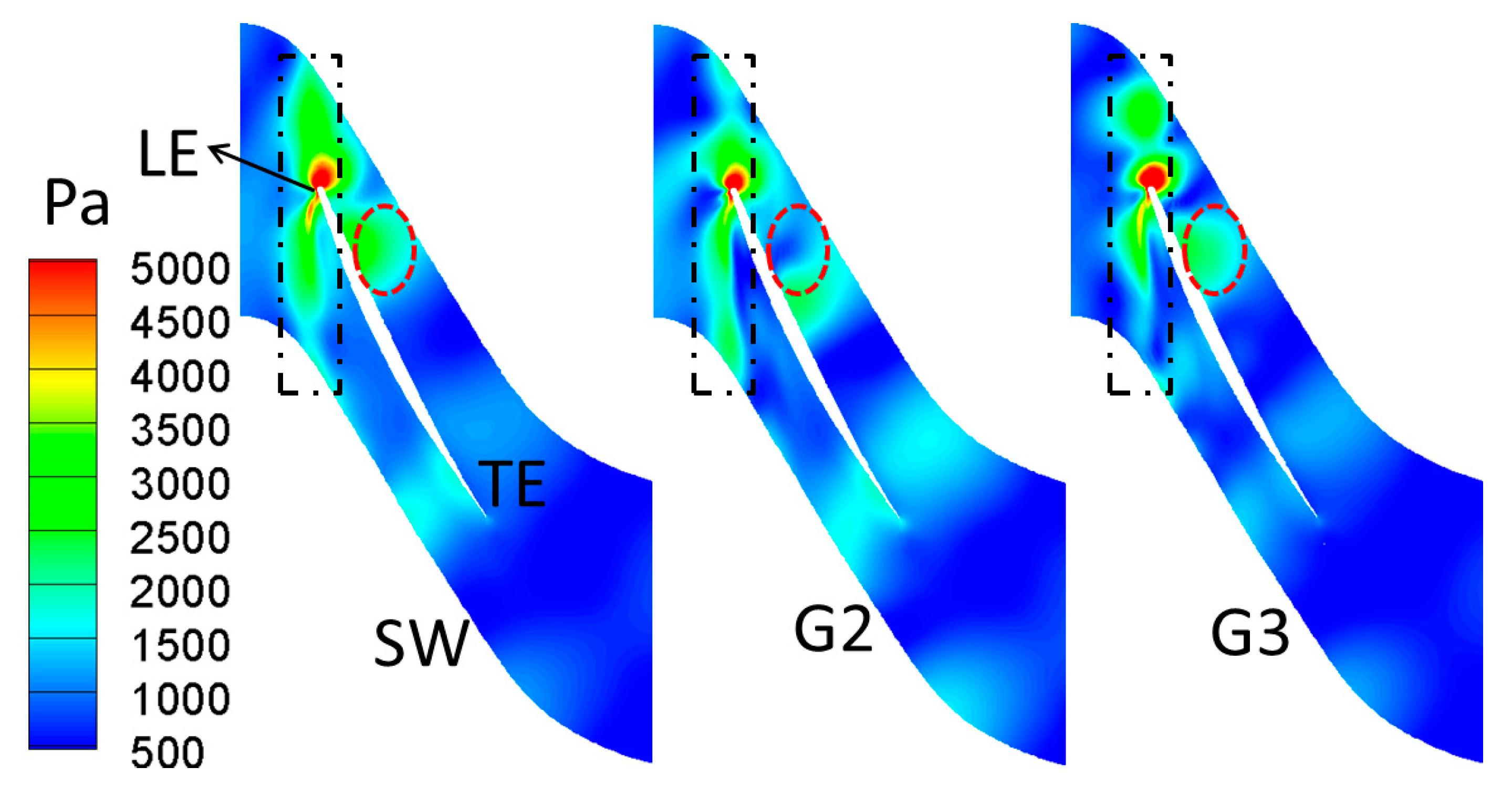
• Parametric studies on the axial location illustrate that the best location (G2) for a single groove of the CRAC should be at about 20% Ca in terms of the SMI (about 4.0%). The interfaces between the TLF and incoming main flow are pushed downstream to different extents by the CTs.
• The locations of the effective CTs are coincident with the range of the high fluctuating region on the blade pressure surface in the SW case and the best scheme of G2 is just located at the position of peak fluctuation. Therefore, the unsteadiness of TLF plays an important role in the stall inception process.
• Both two low frequency components of 0.31 BPF and 0.47 BPF in the SW case are suppressed in the two CTs. The oscillating frequency of the unsteady TLF is changed from 0.74 BPF to 0.82 BPF in G2. Additionally, the amplitudes of the fluctuations on the pressure side are also decreased obviously. Therefore, the vanishing of the low frequency components and the suppression of the TLF unsteadiness are both beneficial to the SMI.
• It is more effective to improve the flow stability by controlling the critical TLF released from near the mid-chord, while the improvement of main TLF released near the blade leading edge is not necessary to achieve the effectiveness of SMI.

Although there are still disagreements in the published literature about how the casing grooves work effectively because the corresponding interaction of the grooves with the tip flow fields is not fully understood, the above findings may offer us a new idea to design the CTs to improve the compressor flow stability. Past research on this compressor has indicated that the TLF from near the mid-chord plays a more important role in the generation of the self-induced unsteadiness of the TLF [37,38]. In the current paper, the result shows that it is more effective to improve the flow stability by controlling the critical TLF released from near the mid-chord. Therefore, it is suggested we should firstly determine which portion of the TLF is the key to originate the self-induced unsteadiness by the analysis of the TLF structures during the grooved CT design process. Then, we should put the emphasis on the control of the critical portion of TLF, i.e., the designated grooves can interact with the critical portion of TLF as much as possible. Finally, the unsteady fluctuations inside are suppressed to some extent and the compressor stall margin is improved by the CTs.

References

1. Vo, H.D. Rotating stall suppression in axial compressors with casing plasma actuation. J. Propuls. Power 2010, 26, 808–818. [Google Scholar] [CrossRef]
2. Choi, M.; Vahdati, M. Recovery process from rotating stall in a fan. J. Propuls. Power 2011, 27, 1161–1168. [Google Scholar] [CrossRef]
3. Furukawa, M.; Saiki, K.; Yamada, K.; Inoue, M. Unsteady flow behavior due to breakdown of tip leakage vortex in an axial compressor rotor at near-stall condition. In Proceedings of the ASME Turbo Expo 2000: Power for Land, Sea, and Air, Munich, Germany, 8–11 May 2000. [Google Scholar]
4. Maerz, J.; Hah, C.; Neise, W. Discussion of an experimental and numerical investigation into the mechanisms of rotating instability. J. Turbomach. 2002, 124, 375. [Google Scholar] [CrossRef]
5. Yamada, K.; Furukawa, M.; Nakano, T.; Inoue, M.; Funazaki, K. Unsteady three-dimensional flow phenomena due to breakdown of tip leakage vortex in a transonic axial compressor rotor. In Proceedings of the ASME Turbo Expo 2004: Power for Land, Sea, and Air, Vienna, Austria, 14–17 June 2004. [Google Scholar]
6. Du, J.; Lin, F.; Zhang, H.; Chen, J. Numerical investigation on the self-induced unsteadiness in tip leakage flow for a transonic fan rotor. J. Turbomach. 2010, 132, 021017. [Google Scholar] [CrossRef]
7. Sakulkaew, S.; Tan, C.S.; Donahoo, E.; Cornelius, C.; Montgomery, M. Compressor efficiency variation with rotor tip gap from vanishing to large clearance. J. Turbomach. 2013, 135, 031030. [Google Scholar] [CrossRef]
8. Cameron, J.D.; Bennington, M.A.; Ross, M.H.; Morris, S.C.; Du, J.; Lin, F.; Chen, J. The Influence of Tip Clearance Momentum Flux on Stall Inception in a High-Speed Axial Compressor. J. Turbomach. 2013, 135, 051005. [Google Scholar] [CrossRef]
9. Du, J.; Lin, F.; Chen, J.; Nie, C.; Biela, C. Flow structures in the tip region for a transonic compressor rotor. J. Turbomach. 2013, 135, 031012. [Google Scholar] [CrossRef]
10. Yamada, K.; Kikuta, H.; Iwakiri, K.; Furukawa, M.; Gunjishima, S. An explanation for flow features of spike-type stall inception in an axial compressor rotor. J. Turbomach. 2013, 135, 021023. [Google Scholar] [CrossRef]
11. Pullan, G.; Young, A.M.; Day, I.J.; Greitzer, E.M.; Spakovszky, Z.S. Origins and structure of spike-type rotating stall. J. Turbomach. 2015, 137, 051007. [Google Scholar] [CrossRef]
12. Day, I.J. Stall, surge, and 75 years of research. J. Turbomach. 2016, 138, 011001. [Google Scholar] [CrossRef]
13. Jothiprasad, G.; Murray, R.C.; Essenhigh, K.; Bennett, G.A.; Saddoughi, S.; Wadia, A.; Breeze-Stringfellow, A. Control of tip-clearance flow in a low speed axial compressor rotor with plasma actuation. J. Turbomach. 2012, 134, 021019. [Google Scholar] [CrossRef]
14. Bae, J.W.; Breuer, K.S.; Tan, C.S. Active control of tip clearance flow in axial compressors. J. Turbomach. 2005, 127, 352–362. [Google Scholar] [CrossRef]
15. Gümmer, V.; Goller, M.; Swoboda, M. Numerical investigation of end wall boundary layer removal on highly loaded axial compressor blade rows. J. Turbomach. 2008, 130, 011015. [Google Scholar] [CrossRef]
16. Jung, Y.J.; Jeon, H.; Jung, Y.; Lee, K.J.; Choi, M. Effects of recessed blade tips on stall margin in a transonic axial compressor. Aerosp. Sci. Technol. 2016, 54, 41–48. [Google Scholar] [CrossRef]
17. Han, S.; Zhong, J. Effect of blade tip winglet on the performance of a highly loaded transonic compressor rotor. Chin. J. Aeronaut. 2016, 29, 653–661. [Google Scholar] [CrossRef]
18. Zhao, S.; Lu, X.; Zhu, J.; Zhang, H. Investigation for the effects of circumferential grooves on the unsteadiness of tip clearance flow to enhance compressor flow instability. In Proceedings of the ASME Turbo Expo 2010: Power for Land, Sea, and Air, Glasgow, UK, 14–18 June 2010. [Google Scholar]
19. Hwang, Y.; Kang, S.H. Numerical study on the effects of casing treatment on unsteadiness of tip leakage flow in an axial compressor. In Proceedings of the ASME Turbo Expo 2012: Turbine Technical Conference and Exposition, Copenhagen, Denmark, 11–15 June 2012. [Google Scholar]
20. Du, J.; Li, J.; Wang, K.; Lin, F.; Nie, C. The Self-induced unsteadiness of tip leakage flow in an axial low-speed compressor with single circumferential casing groove. J. Therm. Sci. 2013, 22, 565–572. [Google Scholar] [CrossRef]
21. Taghavi-Zenouz, R.; Abbasi, S. Alleviation of spike stall in axial compressors utilizing grooved casing treatment. Chin. J. Aeronaut. 2015, 28, 649–658. [Google Scholar] [CrossRef]
22. Juan, D.; Jichao, L.; Lipeng, G.; Feng, L.; Jingyi, C. The impact of casing groove location on stall margin and tip Clearance flow in a low-speed axial compressor. J. Turbomach. 2016, 138, 121007. [Google Scholar] [CrossRef]
23. Liu, L.; Li, J.; Nan, X.; Lin, F. The stall inceptions in an axial compressor with single circumferential groove casing treatment at different axial locations. Aerosp. Sci. Technol. 2016, 59, 145–154. [Google Scholar] [CrossRef]
24. Alone, D.B.; Kumar, S.S.; Shobhavathy, M.T.; Mudipalli, J.R.R.; Pradeep, A.M.; Ramamurthy, S.; Iyengar, V.S. Experimental assessment on effect of lower porosities of bend skewed casing treatment on the performance of high speed compressor stage with tip critical rotor characteristics. Aerosp. Sci. Technol. 2017, 60, 193–202. [Google Scholar] [CrossRef]
25. Sun, D.; Liu, X.; Sun, X. An evaluation approach for the stall margin enhancement with stall precursor-suppressed casing treatment. J. Fluids Eng. 2015, 137, 081102. [Google Scholar] [CrossRef]
26. Dong, X.; Sun, D.; Li, F.; Jin, D.; Gui, X.; Sun, X. Effects of rotating inlet distortion on compressor stability with stall precursor-suppressed casing treatment. J. Fluids Eng. 2015, 137, 111101. [Google Scholar] [CrossRef]
27. Sun, D.; Nie, C.; Liu, X.; Lin, F.; Sun, X. Further investigation on transonic compressor stall margin enhancement with stall precursor-suppressed casing treatment. J. Turbomach. 2016, 138, 021001. [Google Scholar] [CrossRef]
28. Schimming, P. Counter rotating fans—An aircraft propulsion for the future? J. Therm. Sci. 2003, 12, 97–103. [Google Scholar] [CrossRef]
29. Joly, M.; Verstraete, T.; Paniagua, G. Full design of a highly loaded and compact contra-rotating fan using multidisciplinary evolutionary optimization. In Proceedings of the ASME Turbo Expo 2013: Turbine Technical Conference and Exposition, San Antonio, TX, USA, 3–7 June 2013. [Google Scholar]
30. Sharma, P.B.; Jain, Y.P.; Pundhir, D.S. A study of some factors affecting the performance of a contra-rotating axial compressor stage. Proc. Inst. Mech. Eng. Part A 1988, 202, 15–21. [Google Scholar] [CrossRef]
31. Kerrebrock, J.L.; Epstein, A.H.; Merchant, A.A.; Guenette, G.R.; Parker, D.; Onnee, J.F.; Neumayer, F.; Adamczyk, J.J.; Shabbir, A. Design and test of an aspirated counter-rotating fan. J. Turbomach. 2008, 130, 021004. [Google Scholar] [CrossRef]
32. Nouri, H.; Danlos, A.; Ravelet, F.; Bakir, F.; Sarraf, C. Experimental study of the instationary flow between two ducted counter-rotating rotors. J. Eng. Gas Turbines Power 2013, 135, 022601. [Google Scholar] [CrossRef] [Green Version]
33. Mistry, C.; Pradeep, A.M. Influence of circumferential inflow distortion on the performance of a low speed, high aspect ratio contra rotating axial fan. J. Turbomach. 2014, 136, 071009. [Google Scholar] [CrossRef]
34. Shi, L.; Liu, B.; Na, Z.; Wu, X.; Lu, X. Experimental investigation of a counter-rotating compressor with boundary layer suction. Chin. J. Aeronaut. 2015, 28, 1044–1054. [Google Scholar] [CrossRef]
35. Gao, L.; Li, R.; Miao, F.; Cai, Y. Unsteady investigation on tip flow field and rotating stall in counter-rotating axial compressor. J. Eng. Gas Turbines Power 2015, 137, 072603. [Google Scholar] [CrossRef]
36. Wang, Y.; Chen, W.; Wu, C.; Ren, S. Effects of tip clearance size on the performance and tip leakage vortex in dual-rows counter-rotating compressor. Proc. Inst. Mech. Eng. Part G 2015, 229, 1953–1965. [Google Scholar] [CrossRef]
37. Mao, X.; Liu, B. Numerical investigation of the unsteady flow behaviors in a counter-rotating axial compressor. Proc. Inst. Mech. Eng. Part A 2016, 230, 289–301. [Google Scholar] [CrossRef]
38. Mao, X.; Liu, B. Numerical study of the unsteady behaviors and rotating stall inception process in a counter-rotating axial compressor. Proc. Inst. Mech. Eng. Part G 2016, 230, 2716–2727. [Google Scholar] [CrossRef]
39. Pundhir, D.S.; Sharma, P.B.; Chaudhary, K.K. Effect of casing treatment on aerodynamic performance of a contrarotating axial compressor stage. Proc. Inst. Mech. Eng. Part A 1990, 204, 47–55. [Google Scholar] [CrossRef]
40. IGG v8.7, User Manual; NUMECA International: Brussels, Belgium, 2009.
41. FINE/Turbo v8.7, User Manual; NUMECA International: Brussels, Belgium, 2009.
42. Spalart, P.R.; Allmaras, S.R. A one-equation turbulence model for aerodynamic flows. In Proceedings of the 30th Aerospace Sciences Meeting and Exhibit, Reno, NV, USA, 6–9 January 1992. [Google Scholar]
43. Gao, L.; Li, X.; Feng, X.; Liu, B. The effect of tip clearance on the performance of contra-rotating compressor. In Proceedings of the ASME Turbo Expo 2012: Turbine Technical Conference and Exposition, Copenhagen, Denmark, 11–15 June 2012. [Google Scholar]
44. AutoGrid5 v8.7, User Manual; NUMECA International: Brussels, Belgium, 2009.
45. Vo, H.D. Role of Tip Clearance Flow on Axial Compressor; Massachusetts Institute of Technology: Cambridge, MA, USA, 2002. [Google Scholar]
46. Tong, Z.; Lin, F.; Chen, J.; Nie, C.Q. The self-induced unsteadiness of tip leakage vortex and its effect on compressor stall inception. In Proceedings of the ASME Turbo Expo 2007: Power for Land, Sea, and Air, Montreal, QC, Canada, 14–17 May 2007. [Google Scholar]
47. Gourdain, N.; Burguburu, S.; Leboeuf, F.; Miton, H. Numerical simulation of rotating stall in a subsonic compressor. Aerosp. Sci. Technol. 2006, 10, 9–18. [Google Scholar] [CrossRef]
48. Gourdain, N.; Burguburu, S.; Leboeuf, F.; Michon, G.J. Simulation of rotating stall in a whole stage of an axial compressor. Comput. Fluids 2010, 39, 1644–1655. [Google Scholar] [CrossRef]
49. Shabbir, A.; Adamczyk, J.J. Flow mechanism for stall margin improvement due to circumferential casing grooves on axial compressors. J. Turbomach. 2005, 127, 708–717. [Google Scholar] [CrossRef]
50. Chen, H.; Huang, X.; Shi, K.; Fu, S.; Ross, M.; Bennington, M.A.; Cameron, J.D.; Morris, S.C.; McNulty, S.; Wadia, A. A computational fluid dynamics study of circumferential groove casing treatment in a transonic axial compressor. J. Turbomach. 2014, 136, 031003. [Google Scholar] [CrossRef]
Figure 1. The two stage subsonic counter-rotating axial compressor: (a) overall view; (b) enlarged view of the blade rows; and (c) cross-sectional diagram.
Energies 10 01153 g001
Figure 2. Schematic of the circumferential grooved CTs and enlarged view of grid near the groove.
Energies 10 01153 g002
Figure 3. The computational grid of the two rotors.
Energies 10 01153 g003
Figure 4. The comparison of predicted and experimental total pressure ratio curves at design speed.
Energies 10 01153 g004
Figure 5. Absolute total pressure contours on the 90% blade span of IGV and OGV at the near-stall point: (a) IGV; and (b) OGV.
Energies 10 01153 g005
Figure 6. Overall characteristic plot of the CRAC for the SW case and different groove locations.
Energies 10 01153 g006
Figure 7. SMI trend as a function of groove location.
Energies 10 01153 g007
Figure 8. Time-averaged surface streamlines and relative total pressure coefficient contours on the blade tip plane in different CTs.
Energies 10 01153 g008
Figure 9. Time-averaged and pitch-averaged absolute vorticity contours on the meridional plane in the tip region of R2.
Energies 10 01153 g009
Figure 10. Instantaneous static pressure distributions on blade surface at 99% span in different CTs: (a) SW; (b) G2; and (c) G3.
Energies 10 01153 g010
Figure 11. Contours of STD static pressure distribution on the blade surfaces of R2 in different CTs: (a) blade suction surface; and (b) blade pressure surface.
Energies 10 01153 g011
Figure 12. FFT results for numerical probes located near the blade tip along the tip chord in different CTs: (a) SW; (b) G2; and (c) G3.
Energies 10 01153 g012
Figure 13. STD static pressure contours on the middle plane of the grooves perpendicular to the axial direction in different CTs.
Energies 10 01153 g013
Figure 14. Time-averaged 3D flow streamlines released from mid-gap colored with relative Mach number.
Energies 10 01153 g014
Figure 15. Time-averaged 3D flow streamlines released from mid-gap within different chord range colored with relative Mach number: (a) blade leading edge—30% axial chord; and (b) 30–60% axial chord.
Energies 10 01153 g015
Figure 16. STD static pressure contours at 99% blade span of R2 in different CTs.
Energies 10 01153 g016