Switched Control Strategies of Aggregated Commercial HVAC Systems for Demand Response in Smart Grids


Abstract
:1. Introduction
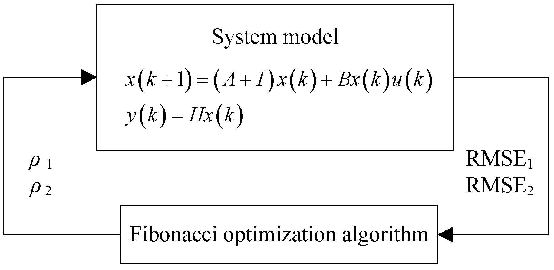
- A discrete-time controller is proposed to adjust the setpoints of the HVAC units and the Fibonacci optimization algorithm is used in [30] to obtain the optimal parameter of the controller.
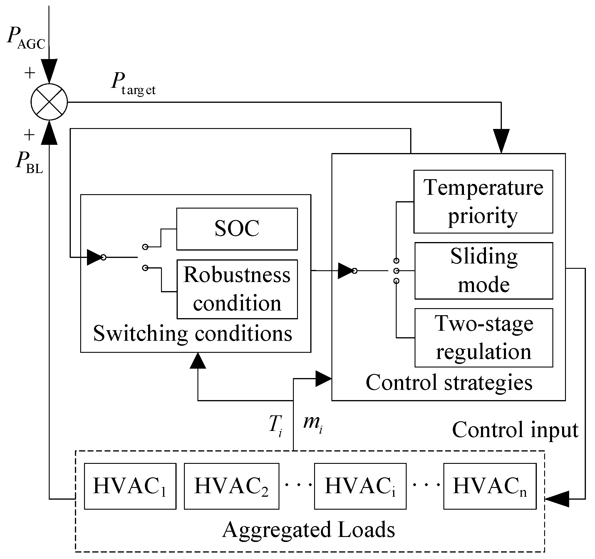
- The switching indices are established before presenting the switched control strategies to track the AGC signal.
- A two-stage regulation strategy is proposed in a single time step to improve the tracking performance of the switched control strategies.
2. System Model and Control Strategies
2.1. Individual HVAC Model
2.2. Typical Control Strategies
2.3. Control Strategy Comparison
2.4. Switched Control Model
- (1)
- First, we design a discrete-time sliding-mode controller to regulate the temperature setpoint and search for the optimal control gain by the Fibonacci optimization algorithm.
- (2)
- Second, we present a pair of switched control strategies according to two switching indices, which are then used to decide which control strategy should be applied across multiple time steps.
- (3)
- Third, we introduce a two-stage regulation in a single control cycle, which means that the loads are regulated twice in one time step. The third switched control strategy is then developed to further improve the tracking performance.
3. Controller Design and Optimization
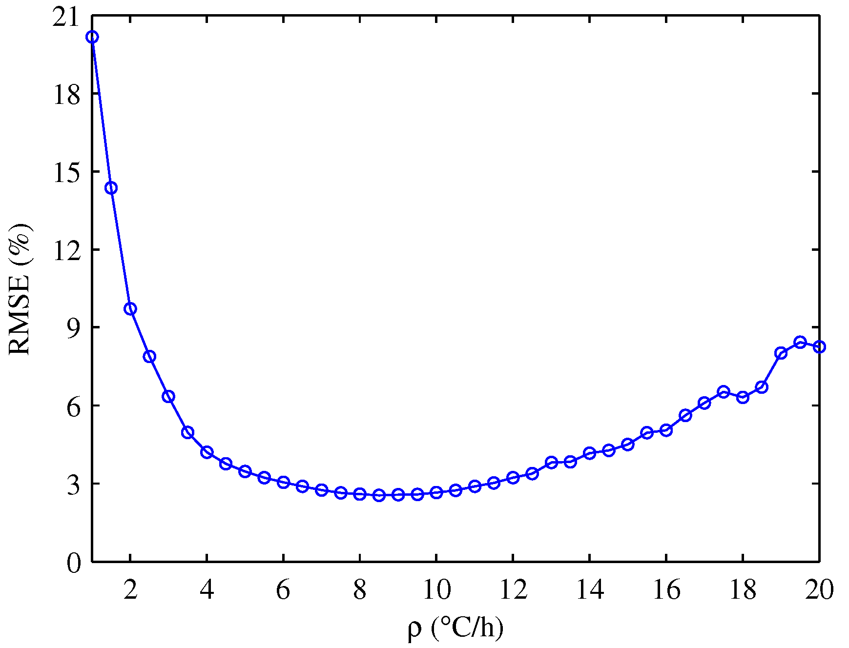
3.1. Parameter Optimization
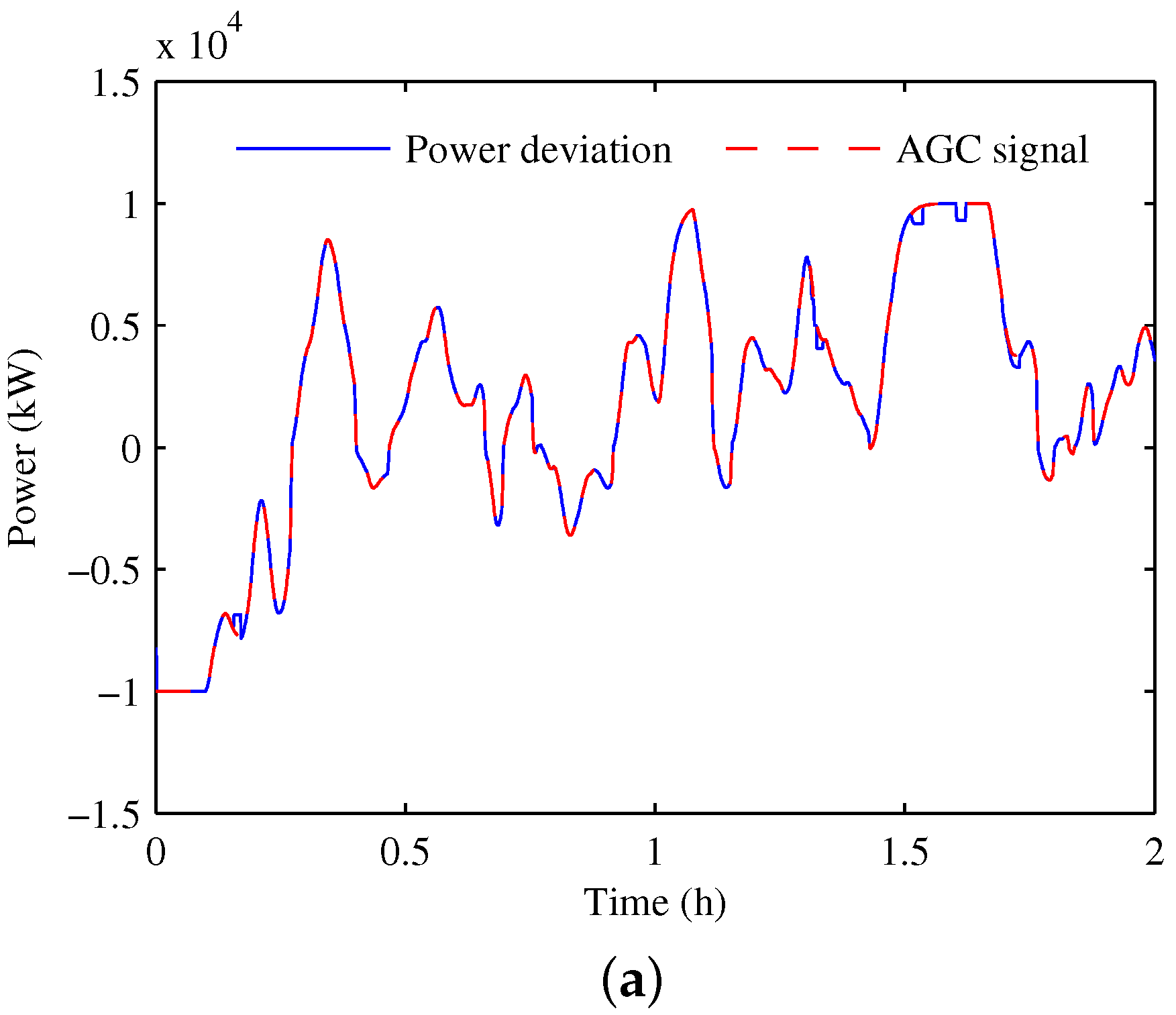
3.2. Switched Control Strategies I and II
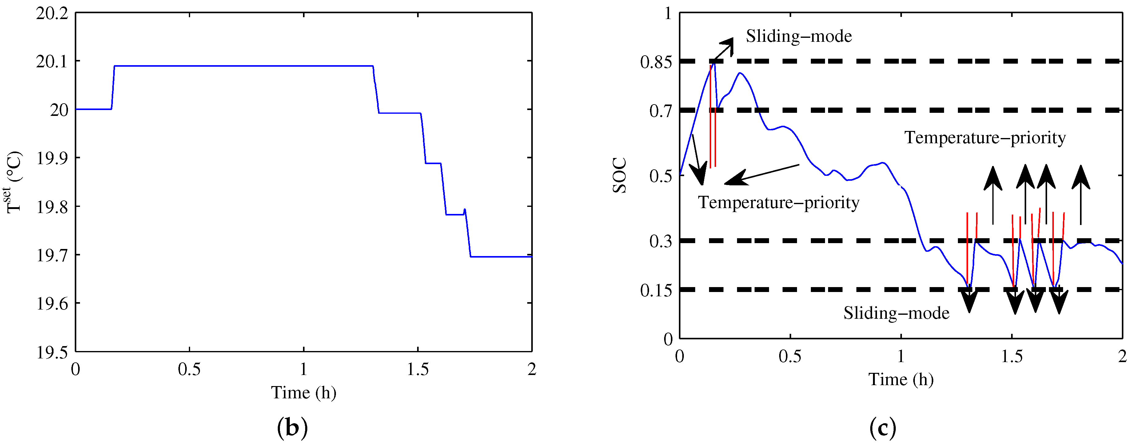
3.3. Switched Control Strategy III
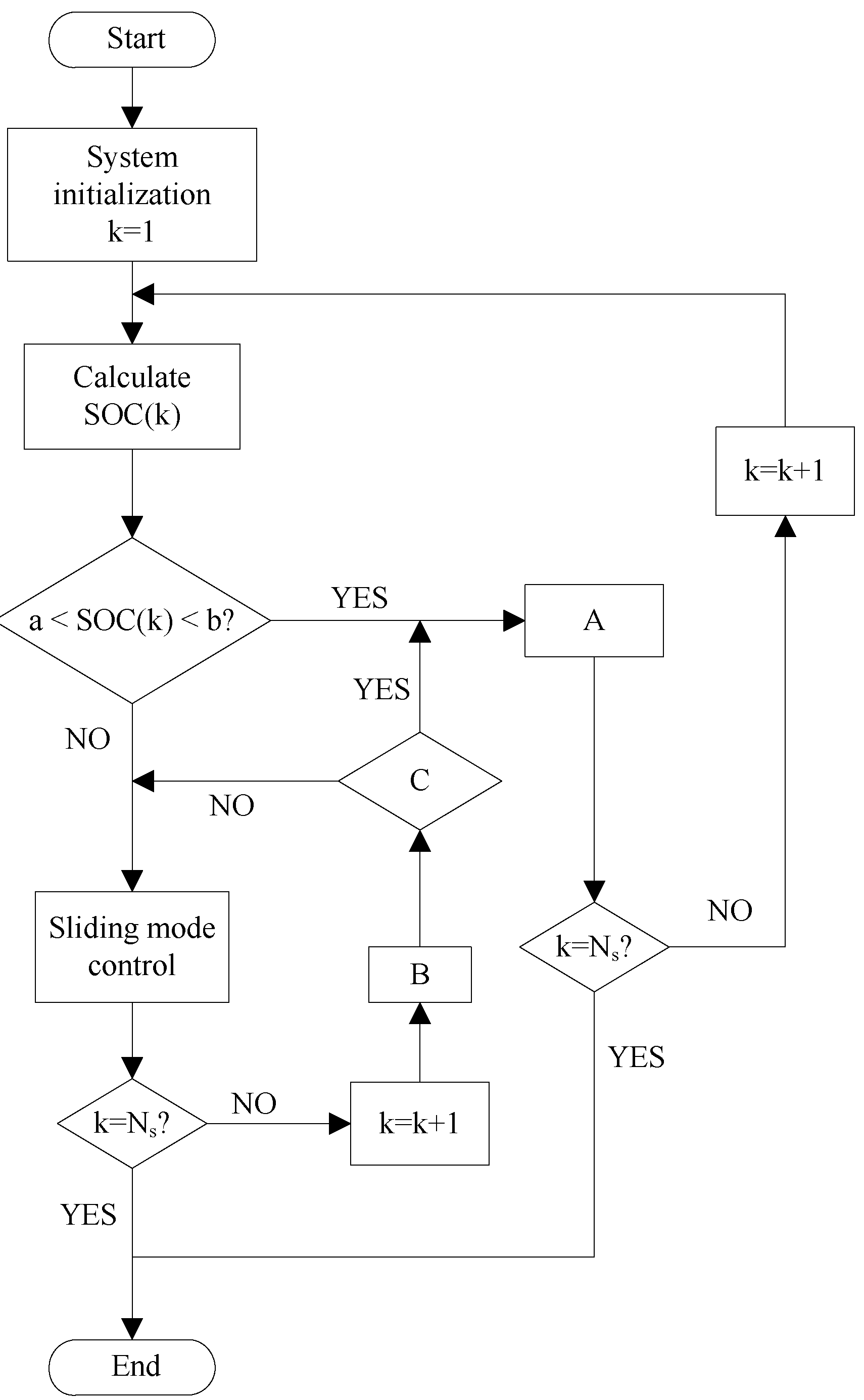
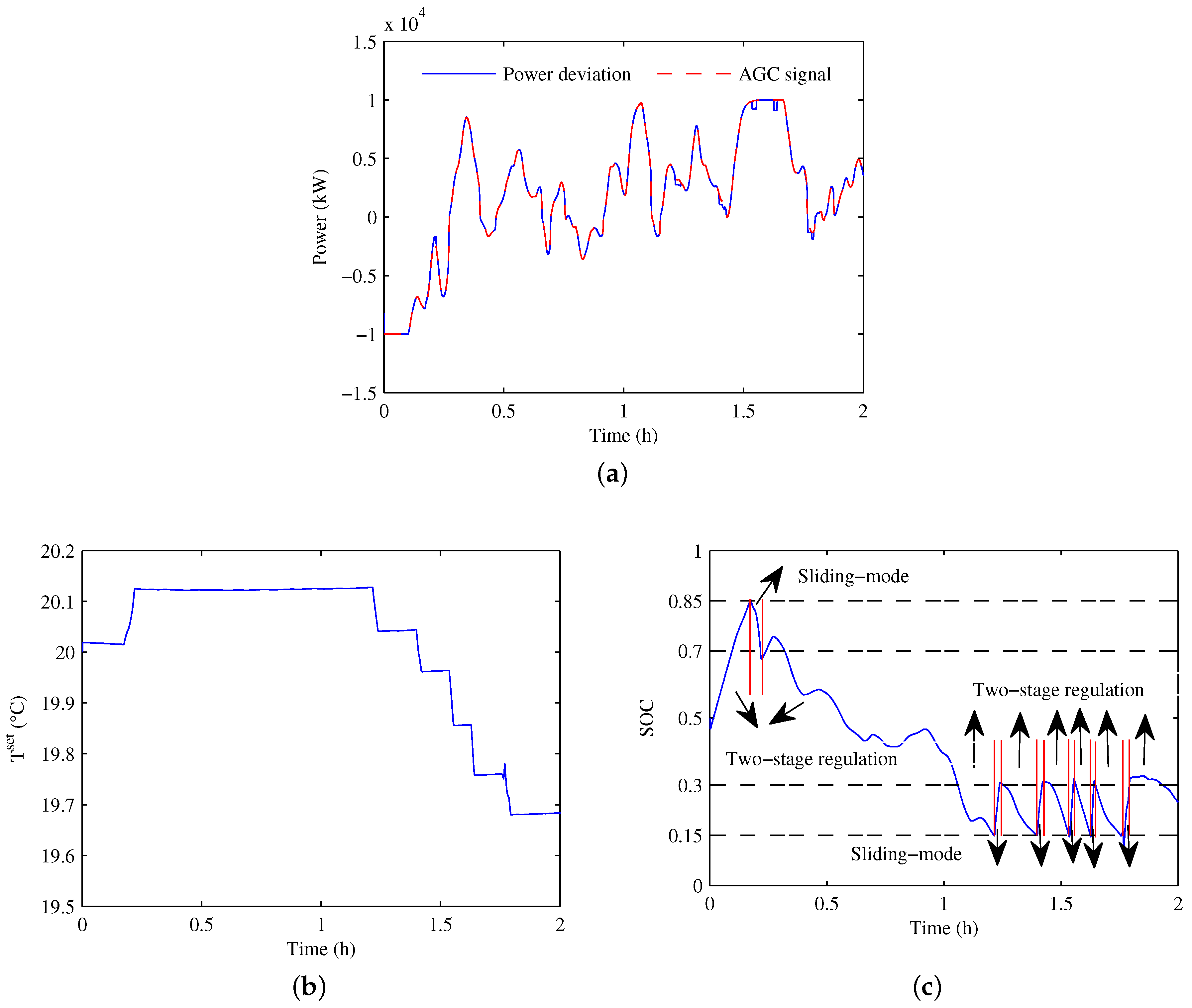
- Utilize the sliding-mode control strategy to track the AGC signal and output the tracking error.
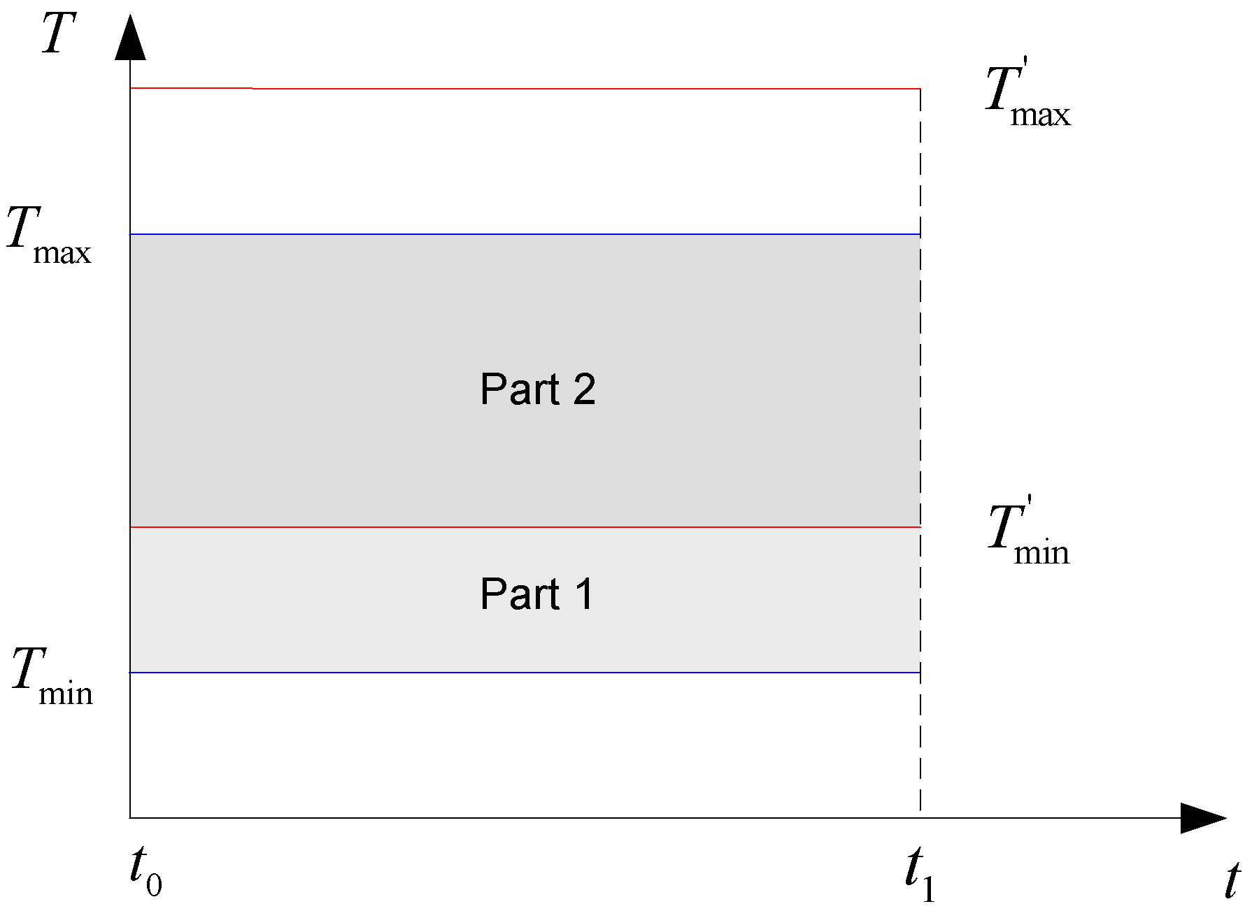
- Divide the loads into Part 1 and Part 2.
- Control the loads in Part 2 based on the temperature-priority control strategy to compensate for the tracking error.
4. Simulation Results
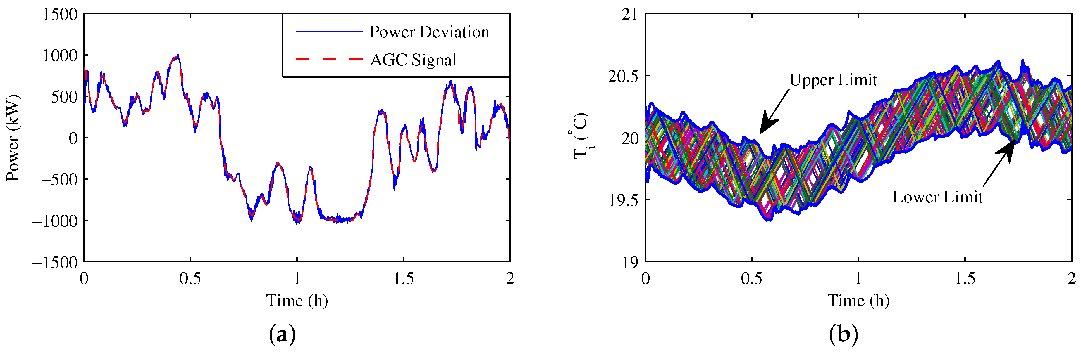
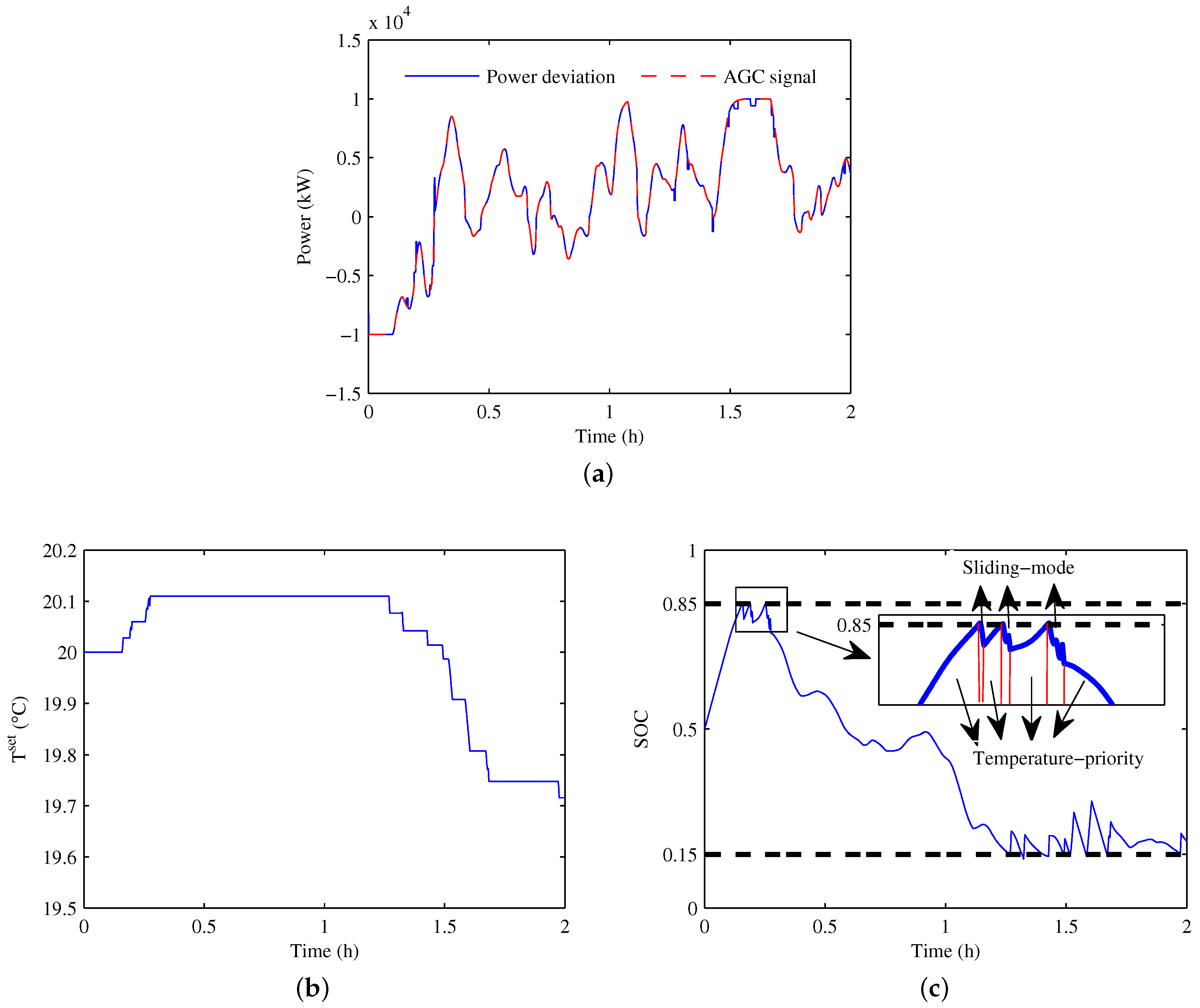
- The tracking performances of the HVAC units under the three switched control strategies are better than they were when using the temperature priority control or the sliding-mode control individually. This is because that the switched control strategies select the appropriate control methods according to the system states. Hence, the disadvantage of each individual method is mitigated. It is observed that the switched control strategies have smaller RMSE and less stepoint changes, and thus they are promising for the frequency regulation.
- On the system operator side, the RMSE value is an important factor. A large RMSE means more reserve capacity is needed, which increases the costs. A small RMSE value stands for good AGC tracking performance, and thus Switched Control Strategy III is the best candidate.
- On the consumer side, the temperature should be maintained in a comfortable region. Thus, the small variation range of the temperature setpoint is preferable. It is observed from Table 4 that the setpoint range of Switched Control Strategy III is the smallest, hence it should be considered first.
- Considering the computing overhead, Switched Control Strategy III is more complex than the others, which is caused by the two-stage regulation. Therefore, to achieve a tradeoff between the RMSE and the computing overhead, Switched Control Strategy I and II are the better choices.
- Considering the wear and tear of the HVAC units, greater numbers of on/off state operations result in more severe wear and tear. The on/off state operations of the sliding-mode control strategy is the least, as shown in Table 4. Hence, to prolong the lifespan of the HVAC units, the sliding-mode control strategy is preferred.
5. Conclusions
Acknowledgments
Author Contributions
Conflicts of Interest
Nomenclature
| T | The internal air temperature (C) |
| The internal mass temperature (C) | |
| The outdoor air temperature (C) | |
| The internal air temperature of i-th HVAC (C) | |
| The on/off state of i-th HVAC | |
| The thermal resistance of i-th HVAC (C/kW) | |
| The thermal capacitance of i-th HVAC (kWh/C) | |
| The energy transfer rate (kW) | |
| The temperature setpoint of i-th HVAC (C) | |
| The upper temperature limit of i-th HVAC (C) | |
| The lower temperature limit of i-th HVAC (C) | |
| The width of the temperature deadband (C) | |
| h | The time step (s) |
| The disturbances | |
| The efficiency coefficient of i-th HVAC | |
| y | The power consumption of aggregated HVAC units (kW) |
| x | The number of loads in corresponding temperature bins |
| R | The average thermal resistance (C/kW) |
| C | The average thermal capacitance (kWh/C) |
| P | The average energy transfer rate (kW) |
| The baseline of power consumption (kW) | |
| The initial average temperature setpoint (C) | |
| The control gain of the sliding-mode controller (C/h) | |
| The boundary layer of the sliding-mode controller (kW) | |
| The power of AGC signal (kW) | |
| The minimum power of AGC signal (kW) | |
| The maximum power of AGC signal (kW) | |
| N | The number of aggregated HVAC units |
| The number of simulation steps | |
| a, b, c, d | The thresholds of SOC |
| n | The number of temperature bins |
Appendix A
| Algorithm A1 Fibonacci optimization |
| Input: The initial optimization interval: ; The final interval width: ; The Fibonacci numbers: |
| Output: Controller gain: ρ* |
| Find the minimum n that satisfies |
| Set |
| Calculate test points: ; ; |
| and ; |
| while () do |
| if then |
| ; ; Update and |
| else |
| ; ; Update and |
| end if |
| end while |
| if then |
| else |
| end if |
| Update and |
| if then |
| else if then |
| else |
| end if |
References
- Du, P.; Lu, N. Appliance Commitment for Household Load Scheduling. IEEE Trans. Power Syst. 2011, 2, 411–419. [Google Scholar] [CrossRef]
- Kirby, B. Ancillary Services: Technical and Commercial Insights. Available online: http://www.science.smith.edu/jcardell/Courses/EGR325/Readings/Ancillary_Services_Kirby.pdf (accessed on 1 November 2013).
- Wen, G.; Hu, G.; Hu, J.; Shi, X. Frequency Regulation of Source-Grid-Load Systems: A Compound Control Strategy. IEEE Trans. Ind. Inf. 2016, 12, 69–78. [Google Scholar]
- Chuang, A.S.; Schwaegerl, C. Ancillary Services for Renewable Integration. In Proceedings of the CIGRE/IEEE PES Joint Symposium Integration of Wide-Scale Renewable Resources Into the Power Delivery System, Calgary, AB, Canada, 29–31 July 2009; p. 1. [Google Scholar]
- Patteeuw, D.; Henze, G.P.; Helsen, L. Comparison of Load Shifting Incentives for Low-energy Buildings with Heat Pumps to Attain Grid Flexibility Benefits. Appl. Energy 2016, 167, 80–92. [Google Scholar] [CrossRef]
- Chassin, D.P.; Stoustrup, J.; Agathoklis, P.; Djilali, N. A New Thermostat for Real-time Price Demand Response: Cost, Comfort and Energy Impacts of Discrete-time Control without Deadband. Appl. Energy 2015, 155, 816–825. [Google Scholar] [CrossRef]
- Lakshmanan, V.; Marinelli, M.; Hu, J.; Bindner, H.W. Provision of Secondary Frequency Control via Demand Response Activation on Thermostatically Controlled Loads: Solutions and Experiences from Denmark. Appl. Energy 2016, 173, 470–480. [Google Scholar] [CrossRef]
- Cole, W.J.; Rhodes, J.D.; Gorman, W.; Perez, K.X.; Webber, M.E.; Edgar, T.F. Community-scale Residential Air Conditioning Control for Effective Grid Management. Appl. Energy 2014, 130, 428–436. [Google Scholar] [CrossRef]
- Callaway, D.S. Tapping the Energy Storage Potential in Electric Loads to Deliver Load Following and Regulation, with Application to Wind Energy. Energy Convers. Manag. 2009, 50, 1389–1400. [Google Scholar] [CrossRef]
- Chong, C.Y.; Malhami, R.P. Statistical Synthesis of Physically Based Load Models with Applications to Cold Load Pickup. IEEE Trans. Power Appar. Syst. 1984, 4, 1621–1628. [Google Scholar] [CrossRef]
- Burger, E.M.; Moura, S.J. Generation Following with Thermostatically Controlled Loads via Alternating Direction Method of Multipliers Sharing Algorithm. Electr. Power Syst. Res. 2017, 146, 141–160. [Google Scholar] [CrossRef]
- Liu, S.; Xie, L.; Cai, W. Cooperative Control of VAV Air-conditioning Systems. In Proceedings of the 31st Chinese Control Conference, Hefei, China, 25–27 July 2012; pp. 6938–6942. [Google Scholar]
- Liu, S.; Long, Y.; Xie, L.; Bayen, A.M. Cooperative Control of Air Flow for HVAC Systems. In Proceedings of the IEEE International Conference on Automation Science and Engineering (CASE 2013), Madison, WI, USA, 17–20 August 2013; pp. 422–427. [Google Scholar]
- Hui, H.; Ding, Y.; Liu, W.; Lin, Y.; Song, Y. Operating Reserve Evaluation of Aggregated Air Conditioners. Appl. Energy 2017, 196, 218–228. [Google Scholar] [CrossRef]
- Ma, K.; Hu, G.; Spanos, C.J. Distributed Energy Consumption Control via Real-Time Pricing Feedback in Smart Grid. IEEE Trans. Control Syst. Technol. 2014, 22, 1907–1914. [Google Scholar]
- Ma, K.; Hu, G.; Spanos, C.J. A Cooperative Demand Response Scheme Using Punishment Mechanism and Application to Industrial Refrigerated Warehouses. IEEE Trans. Ind. Inf. 2015, 99, 1520–1531. [Google Scholar] [CrossRef]
- Ma, K.; Hu, G.; Spanos, C.J. Energy Management Considering Load Operations and Forecast Errors with Application to HVAC Systems. Available online: http://ieeexplore.ieee.org/abstract/document/7458899/ (accessed on 6 June 2016).
- Lu, N.; Chassin, D.P.; Widergren, S.E. Modeling Uncertainties in Aggregated Thermostatically Controlled Loads Using a State Queueing Model. IEEE Tran. Power Syst. 2005, 20, 725–733. [Google Scholar] [CrossRef]
- Lu, N.; Zhang, Y. Design Considerations of a Centralized Load Controller Using Thermostatically Controlled Appliances for Continuous Regulation Reserves. IEEE Trans. Smart Grid 2013, 4, 914–921. [Google Scholar] [CrossRef]
- Lu, N. An Evaluation of the HVAC Load Potential for Providing Load Balancing Service. IEEE Trans. Smart Grid 2012, 3, 1263–1270. [Google Scholar] [CrossRef]
- Vanouni, M.; Lu, N. Improving the Centralized Control of Thermostatically Controlled Appliances by Obtaining the Right Information. IEEE Trans. Smart Grid 2015, 6, 946–948. [Google Scholar] [CrossRef]
- Zhou, Y.; Wang, C.; Wu, J.; Wang, J.; Cheng, M.; Li, G. Optimal Scheduling of Aggregated Thermostatically Controlled Loads with Renewable Generation in the Intraday Electricity Market. Appl. Energy 2017, 188, 456–465. [Google Scholar] [CrossRef]
- Hao, H.; Sanandaji, B.M.; Poolla, K.; Vincent, T.L. Aggregate Flexibility of Thermostatically Controlled Loads. IEEE Trans. Power Syst. 2015, 30, 189–198. [Google Scholar] [CrossRef]
- Yin, R.; Kara, E.C.; Li, Y.; Deforest, N.; Wang, K.; Yong, T.; Stadler, M. Quantifying Flexibility of Commercial and Residential Loads for Demand Response using Setpoint Changes. Appl. Energy 2016, 177, 149–164. [Google Scholar] [CrossRef]
- Perfumo, C.; Kofman, E.; Braslavsky, J.H.; Ward, J.K. Load Management: Model-based Control of Aggregate Power for Populations of Thermostatically Controlled Loads. Energy Convers. Manag. 2012, 55, 36–48. [Google Scholar] [CrossRef]
- Braslavsky, J.H.; Perfumo, C.; Ward, J.K. Model-based Feedback Control of Distributed Air-conditioning Loads for Fast Demand-side Ancillary Services. In Proceedings of the IEEE Conference on Decision and Control, Florence, Italy, 10–13 December 2013; pp. 6274–6279. [Google Scholar]
- Kundu, S.; Sinitsyn, N.; Backhaus, S.; Hiskens, I. Modeling and control of thermostatically controlled loads. Available online: https://arxiv.org/abs/1101.2157 (accessed on 10 May 2013).
- Bashash, S.; Fathy, H.K. Modeling and Control Insights into Demand-side Energy Management through Setpoint Control of Thermostatic Loads. In Proceedings of the American Control Conference (ACC), San Francisco, CA, USA, 29 June–1 July 2011; pp. 4546–4553. [Google Scholar]
- Tindemans, S.H.; Trovato, V.; Strbac, G. Decentralized Control of Thermostatic Loads for Flexible Demand Response. IEEE Trans. Control Syst.Technol. 2015, 23, 1685–1700. [Google Scholar] [CrossRef]
- Chen, B. Optimization Theory and Method; Tsinghua University press: Beijing, China, 1989; pp. 420–433. [Google Scholar]
- Chang, C.Y.; Zhang, W.; Lian, J.; Kalsi, K. Modeling and Control of Aggregated Air Conditioning Loads under Realistic Conditions. In Proceedings of the IEEE PES Innovative Smart Grid Technologies (ISGT), Washington, DC, USA, 24–27 February 2013; pp. 1–6. [Google Scholar]
- Mathieu, J.L.; Callaway, D.S. State Estimation and Control of Heterogeneous Thermostatically Controlled Loads for Load Following. In Proceedings of the 45th Hawaii International Conference on System Science (HICSS), Maui, HI, USA, 4–7 January 2012; pp. 2002–2011. [Google Scholar]
- Bashash, S.; Fathy, H.K. Modeling and Control of Aggregate Air Conditioning Loads for Robust Renewable Power Management. IEEE Trans. Control Syst. Technol. 2013, 21, 1318–1327. [Google Scholar] [CrossRef]
- Mathieu, T.L.; Dyson, M.; Callaway, D.S. Using residential electric loads for fast demand response: The potential resource and revenues, the costs, and policy recommendations. Available online: http://aceee.org/files/proceedings/2012/data/papers/0193-000009.pdf (accessed on 3 October 2015).
- Koch, S.; Mathieu, J.L.; Callaway, D.S. Modeling and control of aggregated heterogeneous thermostatically controlled loads for ancillary services. Available online: https://pdfs.semanticscholar.org/ca5b/e7ee06c6f156bd124e505d5da27eebb90803.pdf (accessed on 23 May 2016).
- Judkoff, R.; Barker, G.; Subbarao, K. Buildings in a Test Tube: Validation of the Short-Term Energy Monitoring (STEM) Method (Preprint). Available online: http://www.nrel.gov/docs/fy01osti/29805.pdf (accessed on 26 January 2016).
- PJM. PJM Normalized Dynamic and Traditional Regulation Signals. Available online: http://www.pjm.com/markets-and-operations/ancillary-services/mktbased-regulation/fast-response-regulation-signal.aspx (accessed on 20 November 2015).
- Ma, K.; Yuan, C.; Liu, Z.; Yang, J.; Guan, X. Hybrid control of aggregated thermostatically controlled loads: step rule, parameter optimisation, parallel and cascade structures. IET Gener. Trans. Distrib. 2016, 10, 4149–4157. [Google Scholar] [CrossRef]


| Parameters | Meanings | Values |
|---|---|---|
| R | Average thermal resistance | 2 C/kW |
| C | Average thermal capacitance | 2 kWh/C |
| P | Average energy transfer rate | 14 kW |
| efficiency coefficient | 2.5 | |
| Initial temperature setpoint | 20 C | |
| Ambient temperature | 32 C | |
| Thermostat deadband | 0.5 C | |
| Control gain | 8.6 C/h | |
| Boundary layer | 200 kW | |
| h | Time step | 4 s |
| Day | 1 | 2 | 3 | 4 | 5 | 6 | 7 | 8 | 9 | 10 |
|---|---|---|---|---|---|---|---|---|---|---|
| (C/h) | 8.95 | 8.39 | 9.43 | 8.39 | 8.60 | 8.08 | 8.39 | 8.94 | 8.60 | 8.39 |
| Control Strategies | Block A | Block B | Block C |
|---|---|---|---|
| Switched Control Strategy I | Temperature-priority control | Calculate in (14) | ? |
| Switched Control Strategy II | Temperature-priority control | Calculate SOC(k) | c < SOC(k) < d? |
| Switched Control Strategy III | Two-stage regulation | Calculate SOC(k) | c < SOC(k) < d? |
| Control Strategies | RMSE | Setpoint Range (C) | The Number of on/off Operations | ||
|---|---|---|---|---|---|
| Average | Maximum | Minimum | |||
| Temperature priority control [23] | 19.15% | 20 | 6710 | 7804 | 5623 |
| Sliding mode control [33] | 2.78% | 19.42∼22.33 | 159 | 211 | 123 |
| Sliding mode control () | 2.51% | 19.41∼22.32 | 159 | 209 | 123 |
| Switched Control Strategy I | 1.59% | 19.64∼22.17 | 299 | 417 | 223 |
| Switched Control Strategy II | 1.15% | 19.61∼22.19 | 307 | 441 | 230 |
| Switched Control Strategy III | 0.94% | 19.66∼22.16 | 363 | 495 | 279 |
© 2017 by the authors. Licensee MDPI, Basel, Switzerland. This article is an open access article distributed under the terms and conditions of the Creative Commons Attribution (CC BY) license (http://creativecommons.org/licenses/by/4.0/).
Share and Cite
Ma, K.; Yuan, C.; Yang, J.; Liu, Z.; Guan, X. Switched Control Strategies of Aggregated Commercial HVAC Systems for Demand Response in Smart Grids. Energies 2017, 10, 953. https://doi.org/10.3390/en10070953
Ma K, Yuan C, Yang J, Liu Z, Guan X. Switched Control Strategies of Aggregated Commercial HVAC Systems for Demand Response in Smart Grids. Energies. 2017; 10(7):953. https://doi.org/10.3390/en10070953
Chicago/Turabian StyleMa, Kai, Chenliang Yuan, Jie Yang, Zhixin Liu, and Xinping Guan. 2017. "Switched Control Strategies of Aggregated Commercial HVAC Systems for Demand Response in Smart Grids" Energies 10, no. 7: 953. https://doi.org/10.3390/en10070953
APA StyleMa, K., Yuan, C., Yang, J., Liu, Z., & Guan, X. (2017). Switched Control Strategies of Aggregated Commercial HVAC Systems for Demand Response in Smart Grids. Energies, 10(7), 953. https://doi.org/10.3390/en10070953