1. Introduction
The importance of the contribution of renewable energies to electric power generation is growing, the three-phase power converters playing a very important role. For these converters, the use of an LCL filter is preferred over an L filter, as the former can provide much less ripple and more harmonic attenuation using smaller passive elements to comply with standards such us IEEE 519-1992 and IEC 61000-3-12. However, the inherent resonance of the LCL filter can produce closed-loop instability [
1,
2,
3,
4].
When using LCL filters in grid-connected power converters, two common control strategies are used [
4,
5,
6,
7,
8]: to sense and control the converter currents, i.e., converter current feedback (CCF) or to sense and control the grid currents directly, i.e., grid current feedback (GCF). The CCF has the advantage of an inherent semiconductor current limiting, with a straightforward over-current protection and a simpler power layout, whereas the over-current protection in the GCF case implies the use of current sensors at both the grid and converter sides.
However, when using CCF, even if the controlled inverter currents are sinusoidal, when grid voltages are distorted, grid currents are distorted, as well. The distortion mechanism is essentially as follows: the distorted grid voltage is applied to the LCL capacitors, which generate currents proportional to the time-derivative of the applied voltages and, hence, amplifying each voltage harmonic proportionally to its frequency. Finally, the distorted capacitor currents are added to the inverter currents to form the distorted grid currents, making the CCF solution worse than the GCF in terms of grid current quality.
As an attempt to overcome the distortion problem of the CCF, the GCF has recently emerged [
9,
10,
11,
12]. It is usually implemented using proportional-integral (PI) controls with the feedforward of the grid-voltage or proportional-resonant (PR) controls with enough bandwidth and the number of resonances to ensure rejection of the grid current harmonics. However, due to the higher resonance peak and phase drop in the GCF loop compared with the CCF loop [
2,
7], if acceptable control bandwidths are to be achieved, the resonance peak has to be strongly damped in GCF schemes. To avoid filter losses, this significant damping is usually carried out by means of active damping (AD) techniques, which basically consists of a proportional feedforward of the LCL capacitors currents [
9,
10,
13,
14,
15,
16,
17]. This increases hardware or software complexity, either if more sensors are used to measure the capacitors currents or if the currents are estimated instead. In contrast, the CCF can achieve a high bandwidth and good stability margins with just a light passive damping, without the need for AD. Hence, the CCF is preferable also in terms of control simplicity.
With the aim to solve the problem of the grid current distortion while keeping the CCF advantages, this paper proposes a capacitive emulation (CE) technique. It consists of adding the distorted capacitor currents to the controlled inverter currents, so that both distorted capacitor and inverter currents cancel each other out on the grid. This method requires an accurate estimation of the grid-induced capacitor currents, to be added to the inverter current reference, and a control strategy capable of tracking all harmonics of the capacitor currents. A simple PI control with grid-voltage feedforward cancellation is used in this paper, which presents a variable group-delay between two and five samples in closed loop, as will be experimentally shown. Thus, this paper proposes also a buffer-based method to get a leading and filtered estimation that compensates for the delay introduced by the control. The filtering method is non-distorting, adapts to grid voltage amplitude and frequency variations and avoids peak currents when a grid voltage sag occurs.
Finally, the paper shows experimentally the effectiveness of the CE technique to reduce the THD of the grid currents in a 10-kVA transformerless grid-connected inverter with CCF and a PI control with grid-voltage feedforward cancellation. The THD (total harmonic distortion) results are compared with those obtained in the same inverter when using GCF and a proportional-resonant (PR) control, showing that with the proposed CCF + CE solution, the output current quality is improved while preserving the advantages of the CCF.
2. Control Scheme
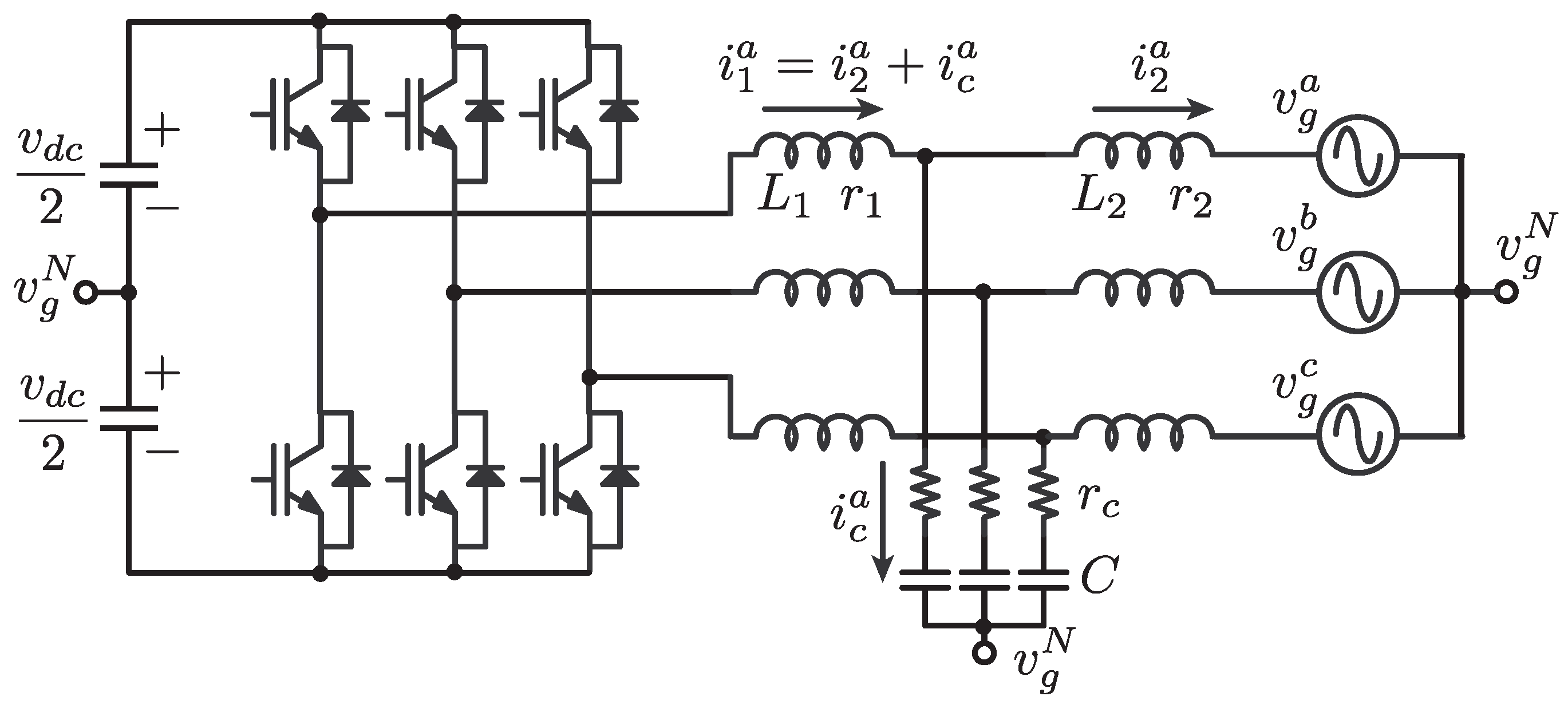
In this section, the current control strategy of the three-phase grid-connected inverter of
Figure 1 when regulating the grid currents (GCF) or the converter currents (CCF) is described in the discrete-time domain considering control delays.
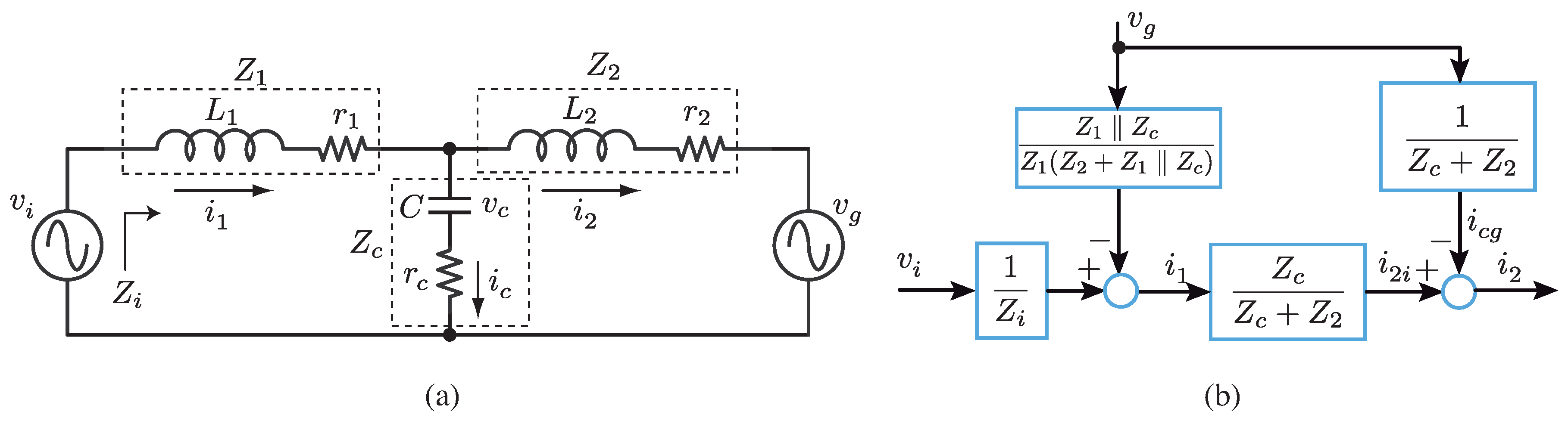
The LCL filter in
Figure 1 can be represented by two decoupled circuits in the
frame as shown in
Figure 2a, where
and
are the grid voltage and inverter averaged voltage, respectively. The inductors
and
are modeled with their inductances
L and series resistances
r. The capacitor series resistance and any possible damping resistance are collected in
.
Figure 2b shows the equivalent block diagram of this filter.
From
Figure 2, the transfer functions from the converter output voltage
to its output current
or to the grid current
are:
being
and
, where the inductor parasitic resistances
and
are neglected for worst case analysis and only
including any passive damping component is considered.
In the case of (
1), as
approach
, by taking
, a nearly pole-zero cancellation can be achieved, reducing the resonance effect, as will be shown in the open-loop gain. This near cancellation or natural attenuation of the resonance is not possible in the case of GCF as shown in Equation (
2).
At low frequencies, below
yields
and
, and the block diagram of
Figure 2b can be simplified by the power stage included in
Figure 3, showing that the LCL filter behaves as an equivalent
L filter with inductance
and series resistance
.
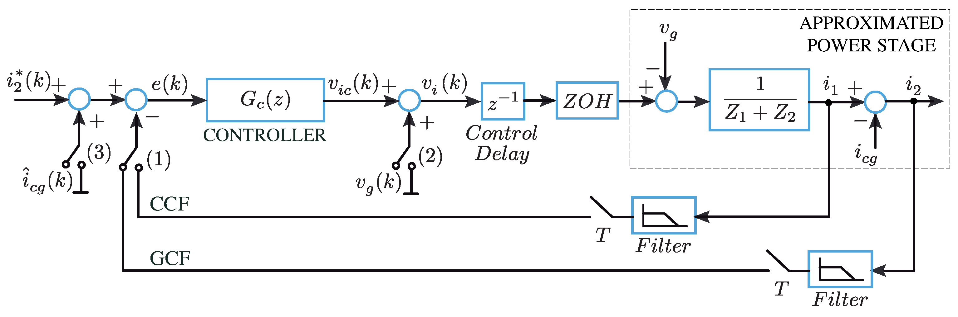
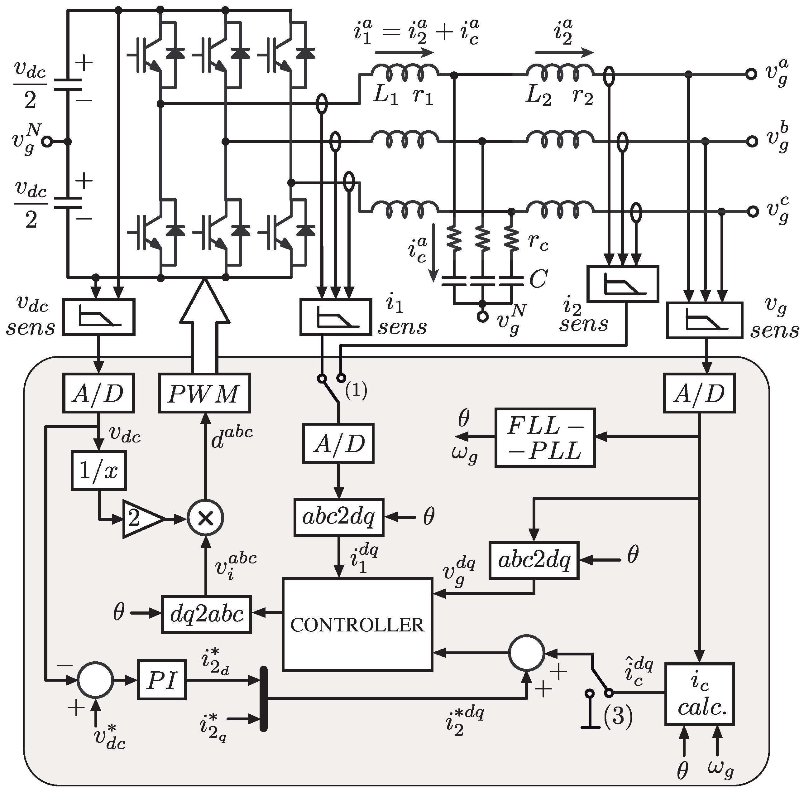
Figure 3 shows an overview of the complete control structure including power plant, anti-aliasing filters, controller and control delay. Switches (1), (2) and (3) represents programming options. With Switch (1), either a GCF or a CCF scheme may be chosen. The grid-voltage feedforward option can be selected according to Switch (2), and Switch (3) adds/removes the CE technique to the control.
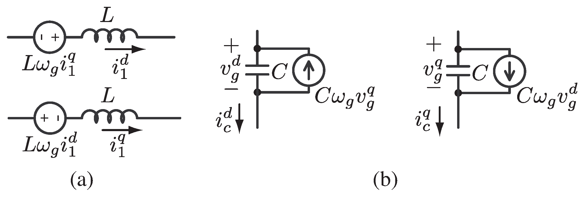
The control is formulated in the
reference frame, where inductors and capacitors are transformed as shown in
Figure 4. Hence, decoupling terms (
for variable
d and
for variable
q) must be added to the controller output in order to decouple the
d and
q current dynamics. These decoupling terms are assumed to be already included in the output signal of the controller
, making the
control diagram of
Figure 3 fully equivalent in the
frame.
For the CCF scheme, a simple PI control with grid-voltage feedforward cancellation is considered. This cancellation is performed adding
to the controller output by turning the Switch (2) ON in
Figure 3. The PI compensator in discretized form is,
where the proportional gain
sets the bandwidth, and the integral gain is
, designed to set the PI’s zero
one decade below the bandwidth.
For the GCF scheme, a proportional-resonant (PR) controller has been used, which provides high gains at certain frequencies (resonant frequencies) eliminating steady state errors at these frequencies [
18,
19]. The PR controller, in the discretized form, is constructed by adding resonant compensators
in parallel to the previous PI controller,
Each resonant compensator
is expressed in terms of an all-pass filter
as [
20]:
being
h the harmonic number,
the resonant gain and:
where
is the resonant frequency and
is the resonant bandwidth.
Another important practical issue that must be taken into account in the analysis are the delays in the control loop that can significantly reduce the stability margins. In general [
21], these delays are due to sensing circuits (anti-aliasing filters of the inverter currents), computational delays (time between the acquisition instant and the total update instant of the control calculations) and the pulse-width modulator (PWM) delay [
18]. In this paper, the anti-aliasing filters have been designed to have a nearly constant group delay, so that they can be modeled as a pure delay term. Computational delays include sampling time and control calculations. In our case, a total control delay of
has been considered.
Multiplying Equation (
1) in discretized form with the PI controller (
3) for CCF, multiplying the discretized form of (
2) with the PR controller (
4) for GCF and adding the control delay of
, the open-loop transfer functions of both feedback schemes are obtained.
For simulation and experimental results, the LCL filter used is specified in
Table 1. The damping coefficient
of the anti-aliasing filters gives minimum variation of the group delay [
22], minimizing the distortion of acquired currents. The programmed PI and PR control parameters are listed in
Table 2, where a high bandwidth (
Hz) has been selected to track the highest number of grid voltage harmonics as possible.
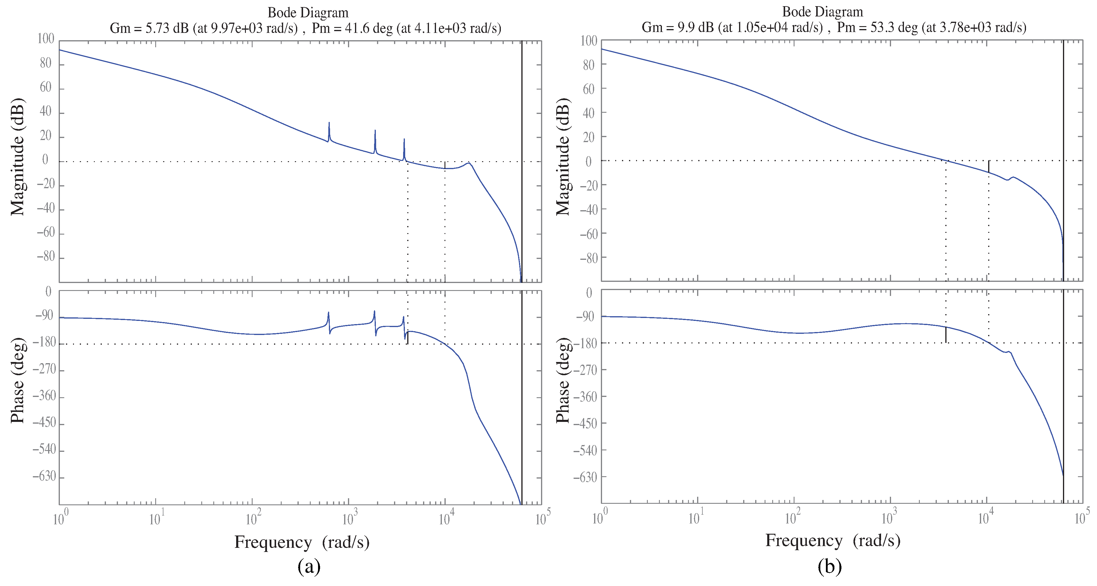
The open-loop Bode diagrams for GCF and CCF strategies obtained from MATLAB are shown in
Figure 5, giving a gain and phase margins of 5.73 dB and 41.6
, respectively, for the GCF and 9.9 dB and 53.3
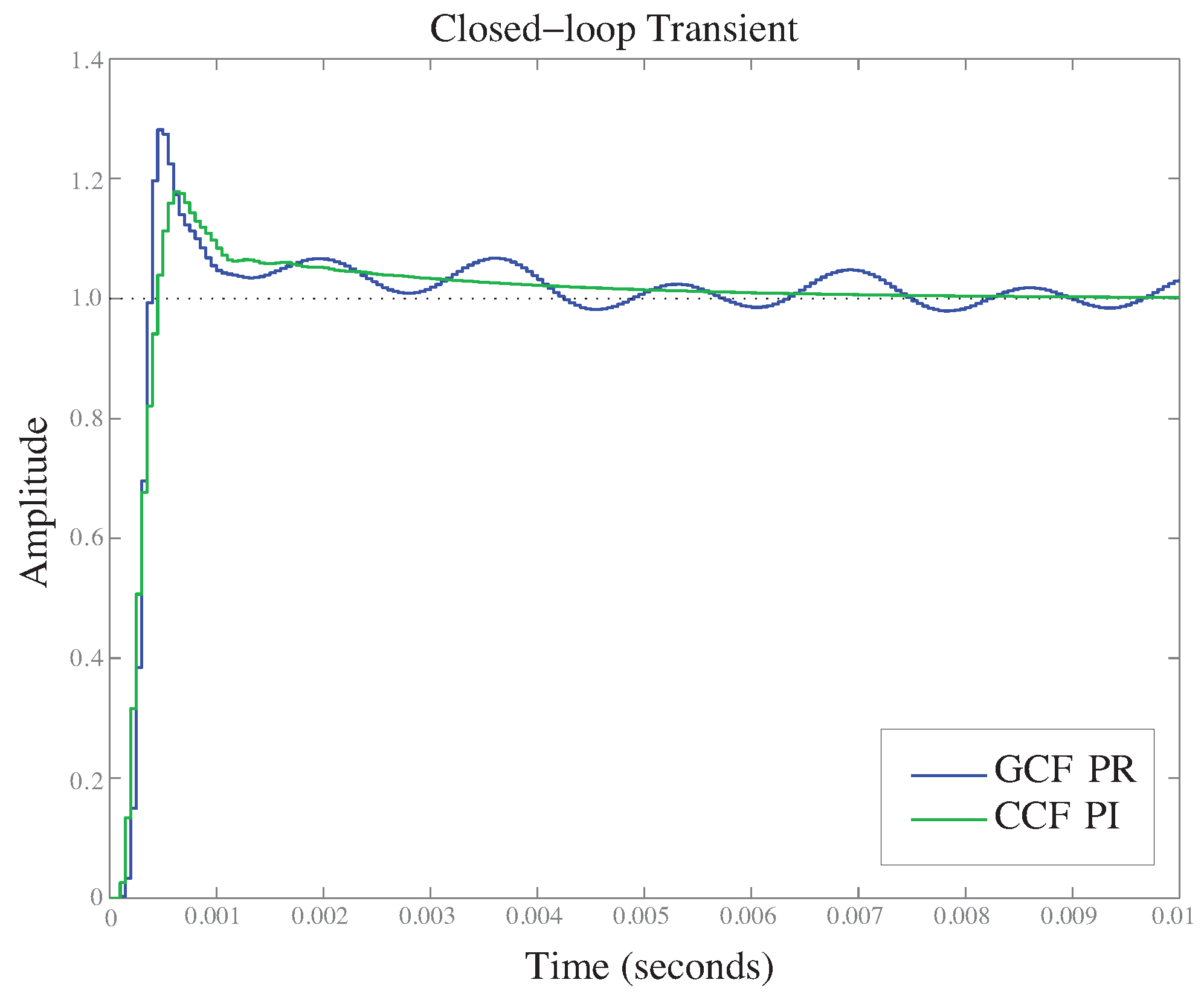
for the CCF. The closed-loop step response is shown in
Figure 6 giving a better response in the CCF case, in accordance with the obtained stability margins and the above explanation.
3. Principles and Limitations of the Capacitive Emulation
Figure 7 shows the simplified closed-loop CCF scheme in the
reference frame. We assume the converter can generate current harmonics on
in a given bandwidth, while
shows all of its harmonic content. By the superposition principle, the line current
is the sum of that generated by
with a short-circuited grid, named
in
Figure 2b, and that generated by the grid voltage when the converter is switched off (
), named
in
Figure 2b. This second term is the distorting capacitive current, the main distortion source affecting the grid current when using CCF with LCL filters. From this analysis, we can affirm that:
The grid voltage harmonics below the resonance -C are applied over the LCL capacitors without attenuation, generating current distortion by capacitive differentiation. The grid voltage harmonics around the resonance can be amplified if no damping method (active or passive) is implemented.
Only the generated harmonics on below the resonance -C are fed to the grid, and therefore, only these harmonics can cancel the distorting capacitive current on the grid.
The capacitor current harmonics below the resonance -C (including the fundamental) are distorting capacitive harmonics.
Hence, the CE method can cancel, at best, the distorting harmonics up to the
-
C resonance. Within this frequency interval, the distorting capacitive current matches the capacitor current and can be expressed in the
frame as (see
Figure 4)
where
is the grid angular frequency and
.
The proposed CE method consists of adding an estimation of the distorting current
to the inverter current reference (
Figure 3):
This estimation has to be ahead to compensate for the closed-loop delay of the current control.
Next, it will be shown that the CE technique requires a grid-voltage feedforward cancellation. In
Figure 3, with Switch (1) in CCF mode, Switch (2) OFF and Switch (3) ON, the current harmonic tracking error in the
frame yields:
where
H is the loop-gain represented in
Figure 5b and
, being
the current reference for the fundamental frequency. If a perfect grid-voltage feedforward is performed,
in Equation (
10) is zero. Without grid-voltage feedforward, the contribution of
to the error can be much higher than the contribution of the reference
. For instance, if we have a grid-voltage distortion of 1.6% for the fifth harmonic (
V
), the distorting capacitor current is
17.5 mA
and
8.3 A
. That is, the current error is much higher when grid-voltage feedforward is not used. In general, (
10) can be written as
where:
being
, and
indicates the amplitude of the feedforward residue (
= 0 represents a perfect feedforward, and
= 1 represents the lack of feedforward).
Figure 8 represents
as a function of the harmonic number below the crossover frequency (13th harmonic) for
= 0 and
= 1, which indicates that the grid-voltage feedforward is necessary for the CE method to compensate the harmonics up to the crossover frequency. However, this is not a drawback, since the acquisition of the grid voltages is necessary for grid synchronization and for calculating the current reference of the CE method.
In case of weak networks, with a relatively large , the attenuation of the switching harmonics is facilitated by this bigger inductance, whereby a smaller capacitor C is normally installed in the LCL filter. Thus, the control can maintain the same bandwidth, and the CE method can still be applied, although it is less necessary because the harmonics generated by the capacitor are of a smaller amplitude.
4. Distorting Current Estimation
The distorting capacitor current estimation
, in the
reference frame, can be calculated as indicated by (
8). This estimation has the advantage of not requiring additional sensors, but it contains derivative terms that generate noise and that have to be filtered. Moreover, this estimation has to be ahead to compensate for the current control delay (between two and five sampling periods), the voltage sensing delay and the reference calculation delay.
We propose to implement this derivative with a small phase lag (a group delay of approximately 0.6 sampling periods) by:
where
is the discrete derivative of
. This differentiator has been obtained by Tustin discretization of the system
, which presents a pole at half the Nyquist frequency.
According to (
8), the distorting current in the
frame can be calculated as:
To filter this noisy estimation, a non-distorting buffer-based technique is proposed. Two constant-size arrays (for
d and
q coordinates) store the
filtered values of the estimation
. Each noisy estimation
calculated using (
13) is averaged with the filtered value stored at the writing index
position:
where
,
and
is the grid voltage angle given by a phase-locked loop (PLL). This is a very simple programming algorithm and offers a first order filtering for each of the 400 array positions. As it filters each array position instead of the whole signal, the result is a waveform without harmonic distortion. Values for
a around 0.9 give satisfactory filtering and adaptation to grid frequency variations. Moreover, the filtering removes any peak generated by (
13) when a voltage sag occurs.
A leading estimation
samples ahead is achieved by reading at the index position
, being:
where the function rem() is the remainder after division, and
is obtained by means of a frequency-locked loop (FLL) algorithm [
23].
Figure 9 shows, in the
frame, the filtered distorting current estimation when the converter is switched off and when it operates at nominal power. An exaggerated number of advance samples
has been programmed to better appreciate the shifting effect.
5. Experimental Results
A 10-kVA transformerless back-to-back converter was built to assess the CE strategy when using CCF and to compare it with a GCF strategy. The rectifier regulates the DC-bus voltage to 800 V, while the inverter solves the current control and the CE method. Two intelligent power modules IPM-PS22A79 from Mitsubishi (Tokyo, Japan) were used.
The DC-bus capacitance was built with four 470
F/450 V capacitors, to reach up to 900 V. The current sensing was implemented using the Hall effect sensors LTS 15-NP (LEM, Geneva, Switzerland) and the grid voltage and DC-voltage sensing using the LV25-P (LEM, Geneva, Switzerland). The LCL filter used at the inverter side is specified in
Table 1. The grid-connected inverter including the PI with grid-voltage feedforward or the PR controller is shown in
Figure 10.
The control was programmed in the Renesas floating point microcontroller R5F5630EDDFB (Renesas Electronics Corporation, Tokyo, Japan). A sampling frequency of 20 kHz was used with a center-aligned PWM pattern. The grid synchronization was carried out by means of an FLL-PLL [
23]. The FLL gives an accurate measure of the grid frequency
, which is used in (
13) and (
15), and to adapt the resonant frequencies
of the PR control in (
7).
The programmed PI and PR control parameters are listed in
Table 2. The proportional gain
sets the bandwidth, and the integral gain
sets the PI’s zero
one decade below the bandwidth. The resonant compensators were tuned experimentally. Starting from the PI configuration, the power spectral density of the grid current
was measured, identifying the following dominant harmonics: 3rd, 7th, 13th and 15th (positive sequence) and 5th, 11th and 17th (negative sequence). To cancel the seventh and 13th positive sequence harmonics, resonant compensators in the
frame for
are required, which in turn cancel the negative sequence fifth and 11th [
24]. Another resonant was added for
to cancel the third harmonic and to remove any fundamental negative sequence.
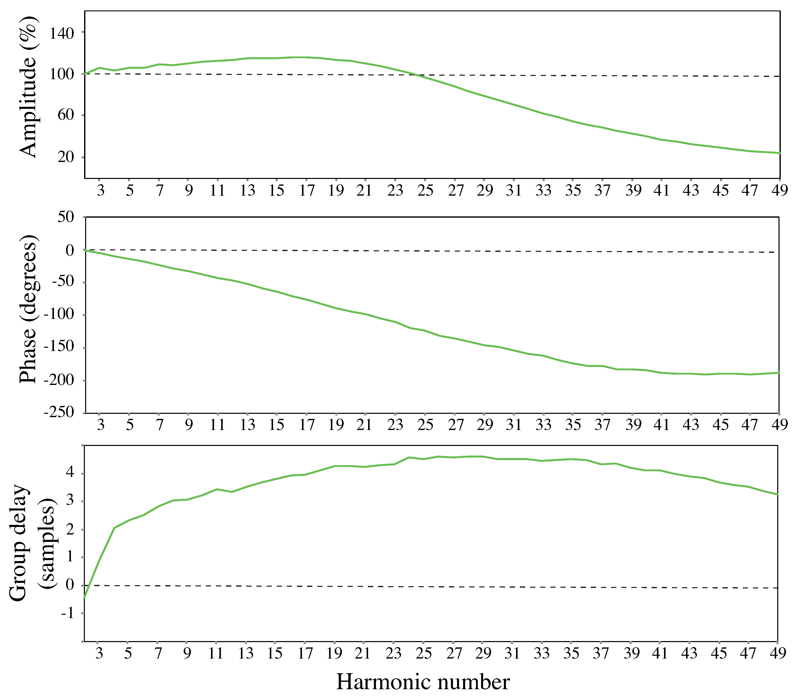
In order to study the group delay of the used PI control with the CCF scheme,
Figure 11 shows the experimental closed-loop response of the system. These results were obtained by programming the current references:
with
A,
A and sweeping for
. The amplitude and phase
of the resulting harmonic on
were measured using the Power & Quality Analyzer CA8384B from Chauvin Arnoux (Paris, France). In order to get delay measurements
referred to the reference harmonic (
16), which is in phase with the grid voltage, both fundamental voltage and current have to be perfectly in phase. This is achieved by adjusting the appropriate value of
before starting the measurements. The group delay was approximated by
samples, being
the measured closed-loop phase in radians. A group delay between two and five samples has been experimentally obtained.
Figure 12a,b is intended to compare the line current quality obtained with the proposed CCF + CE technique and the GCF technique.
Figure 12a shows the grid current waveform and its spectral density at full active power with GCF, giving a THD around 1.3%.
Figure 12b shows the grid current waveform and its spectral density at full active power with CCF + CE, giving a THD around 0.7%. A reduction of THD higher than the 45% is achieved.
Hereafter, the experimental results are focused on the performance of the CCF scheme with PI control and grid-voltage feedforward.
Figure 13 gives the line current THD variation with the number of estimation leading samples when using the CCF and the CE technique, showing that an optimal delay compensation is achieved with six leading samples for all currents levels, i.e.,
= 6 will be considered in Equation (
15).
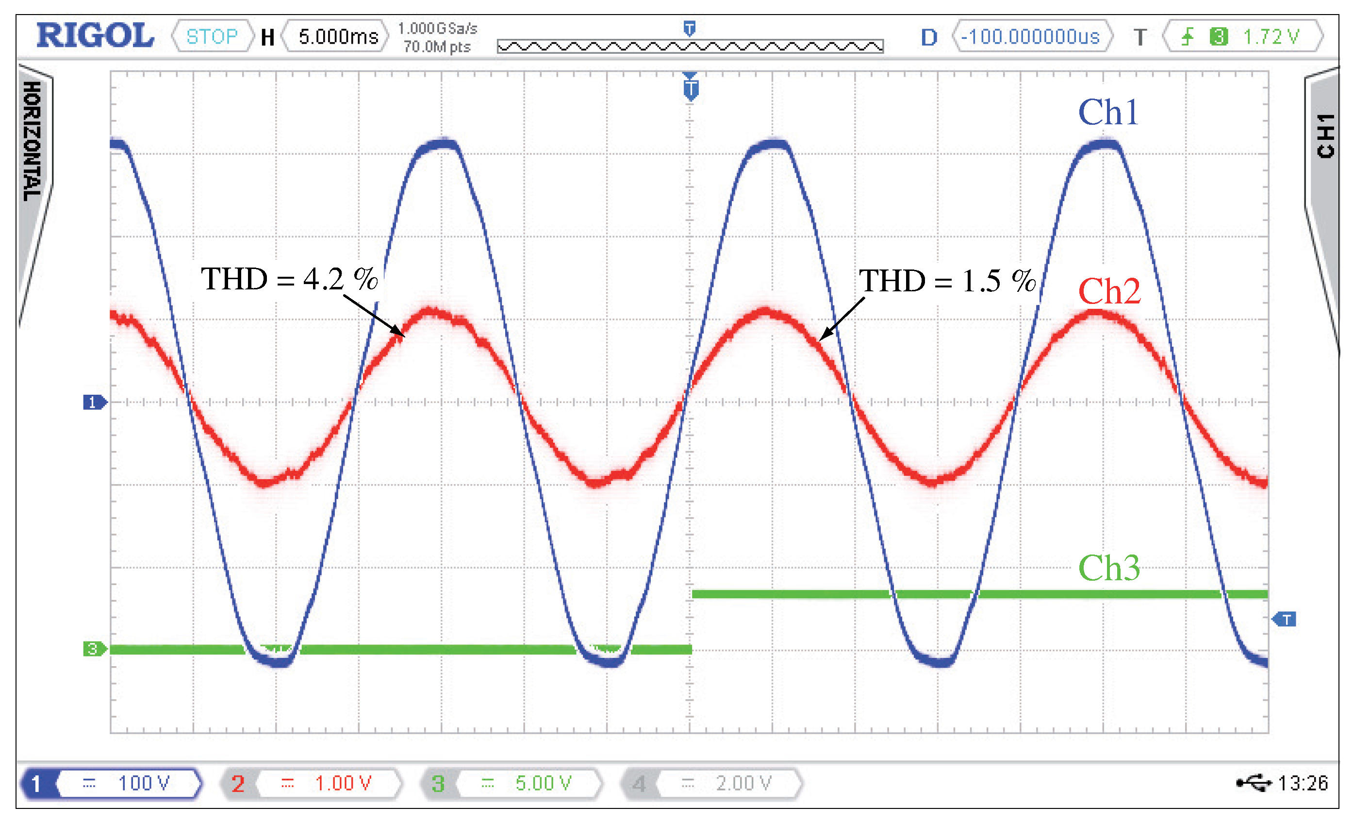
Figure 14 illustrates the effect of using or not the CE strategy. At half the nominal power, the grid current THD is 4.2% without CE, and it reduces to 1.5% with CE. A reduction of THD around 64% is achieved.
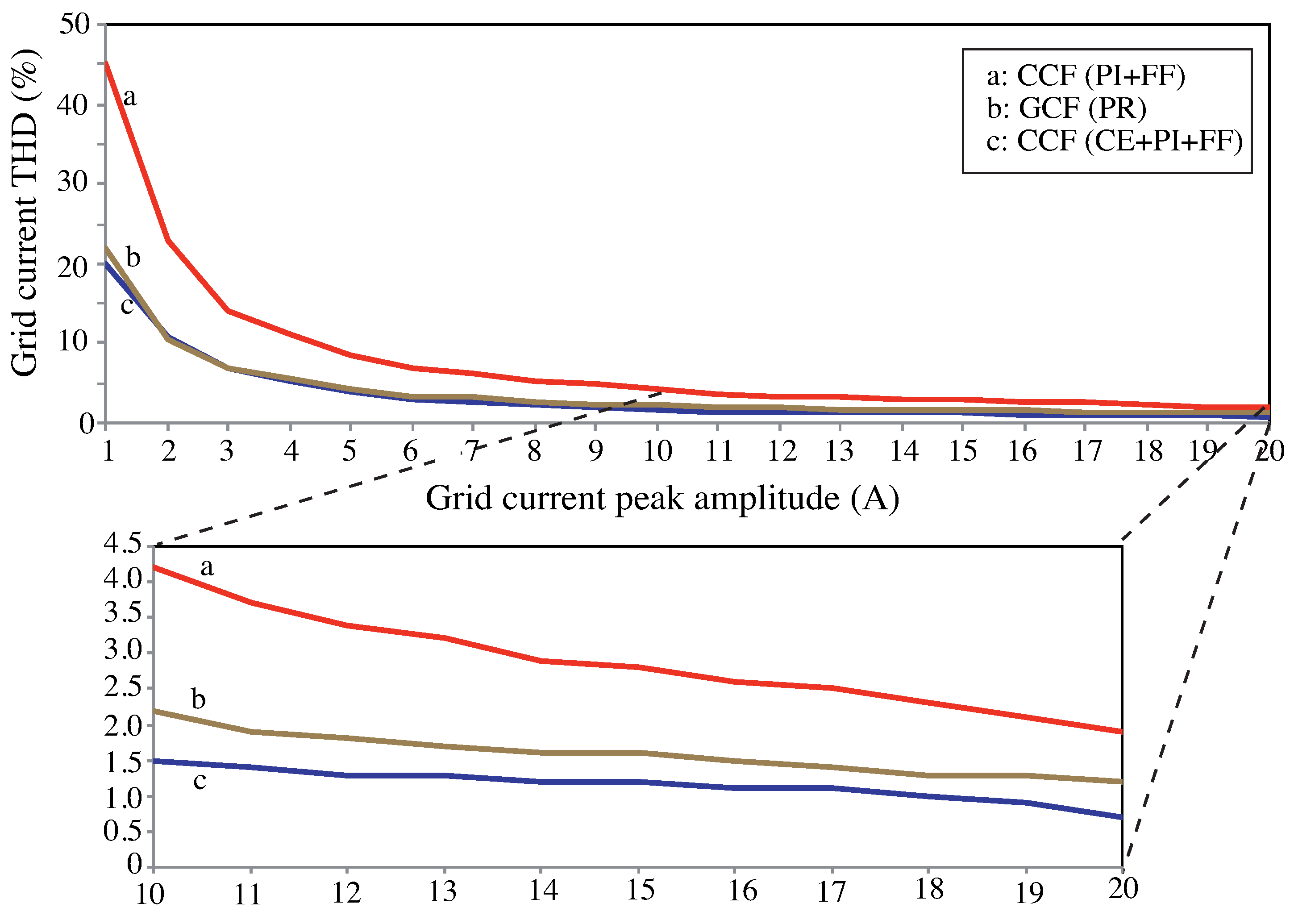
Finally, in order to present a full comparative study,
Figure 15 summarizes the grid current THD for the CCF scheme with and without the CE technique and the GCF scheme with a PR control. Although the GCF achieves very low THD levels around
% at nominal power, better than the CCF with no CE (1.9% at nominal power), the bets results are obtained with the proposed CE technique in CCF, which lowers the THD down to 0.7%.


