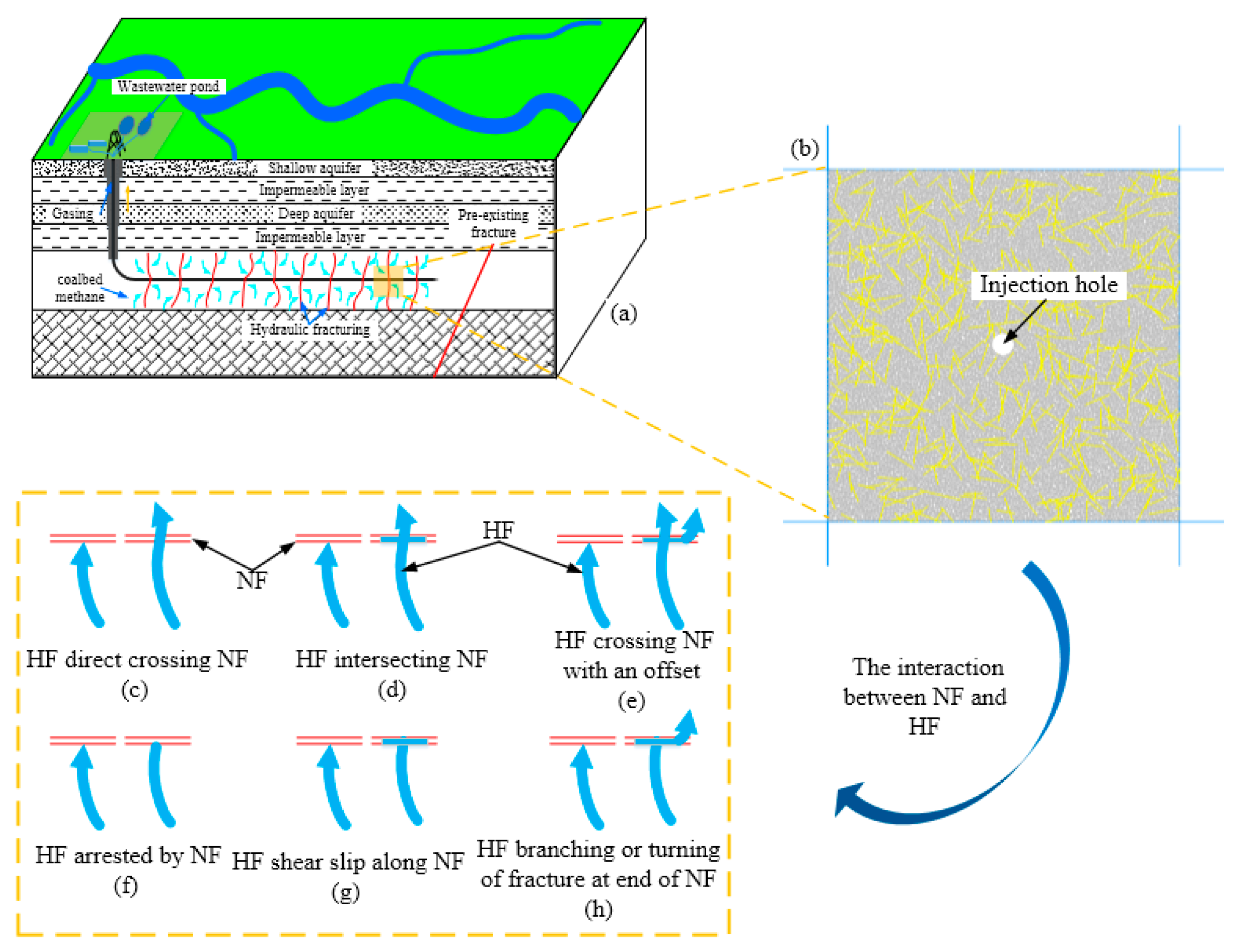
Figure 1.
Geometry of a hydraulic fracture network (HFN) depicting various scenarios of interaction with natural fractures (NFs).
Figure 1.
Geometry of a hydraulic fracture network (HFN) depicting various scenarios of interaction with natural fractures (NFs).
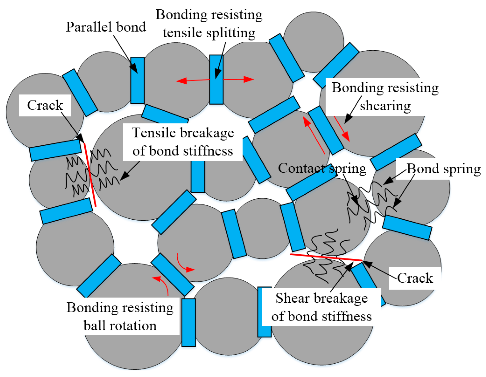
Figure 2.
The parallel bond and its breaks of inter-particle bond in SRM [
32].
Figure 2.
The parallel bond and its breaks of inter-particle bond in SRM [
32].
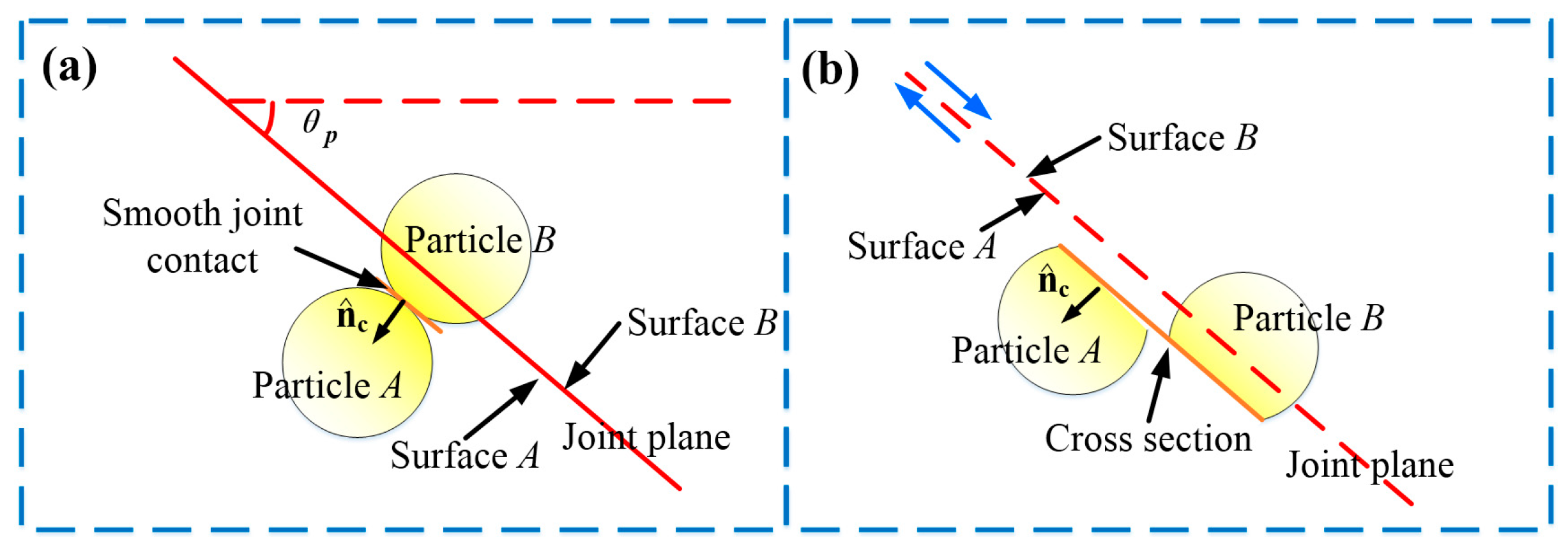
Figure 3.
Smooth joint (SJ) contact model in two dimensions.
Figure 3.
Smooth joint (SJ) contact model in two dimensions.
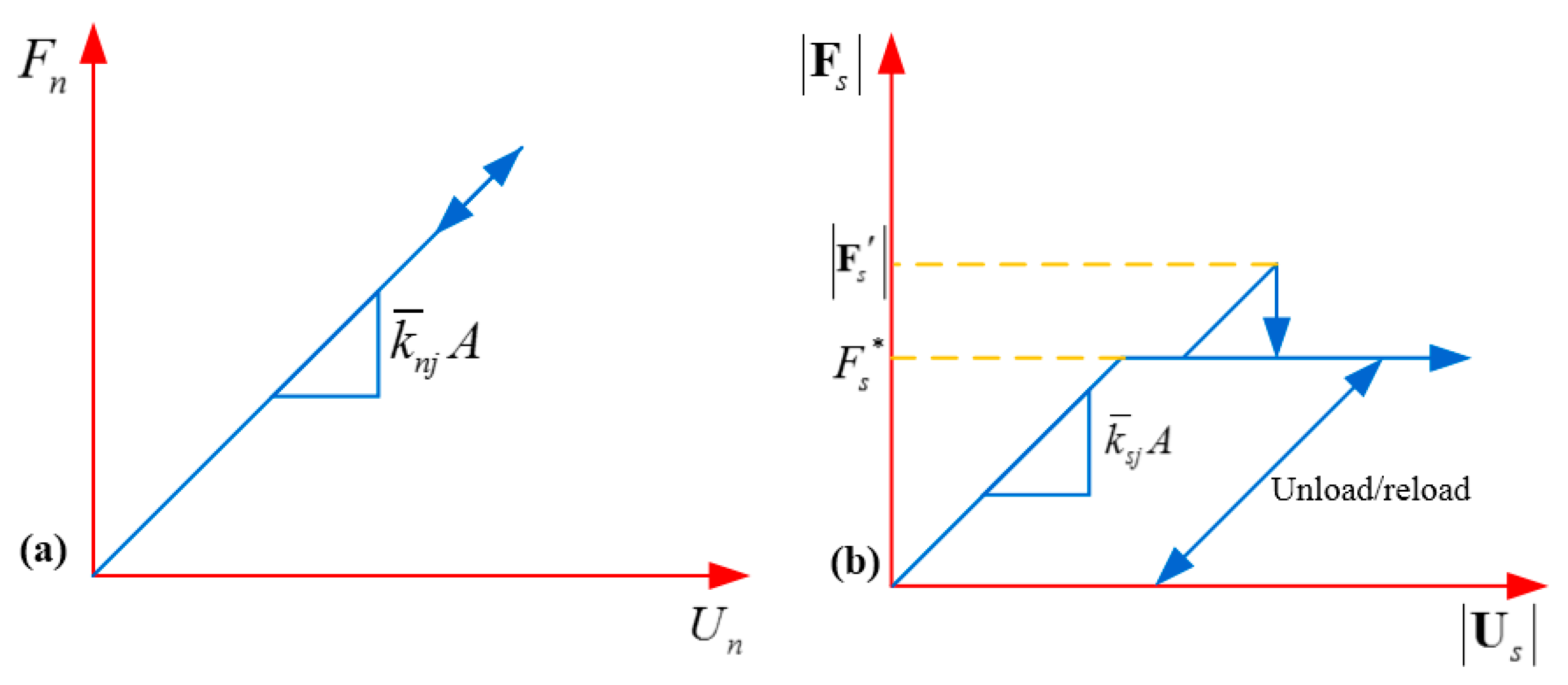
Figure 4.
Smooth joint force-displacement law (a) normal force versus normal displacement; (b) shear force versus shear displacement.
Figure 4.
Smooth joint force-displacement law (a) normal force versus normal displacement; (b) shear force versus shear displacement.
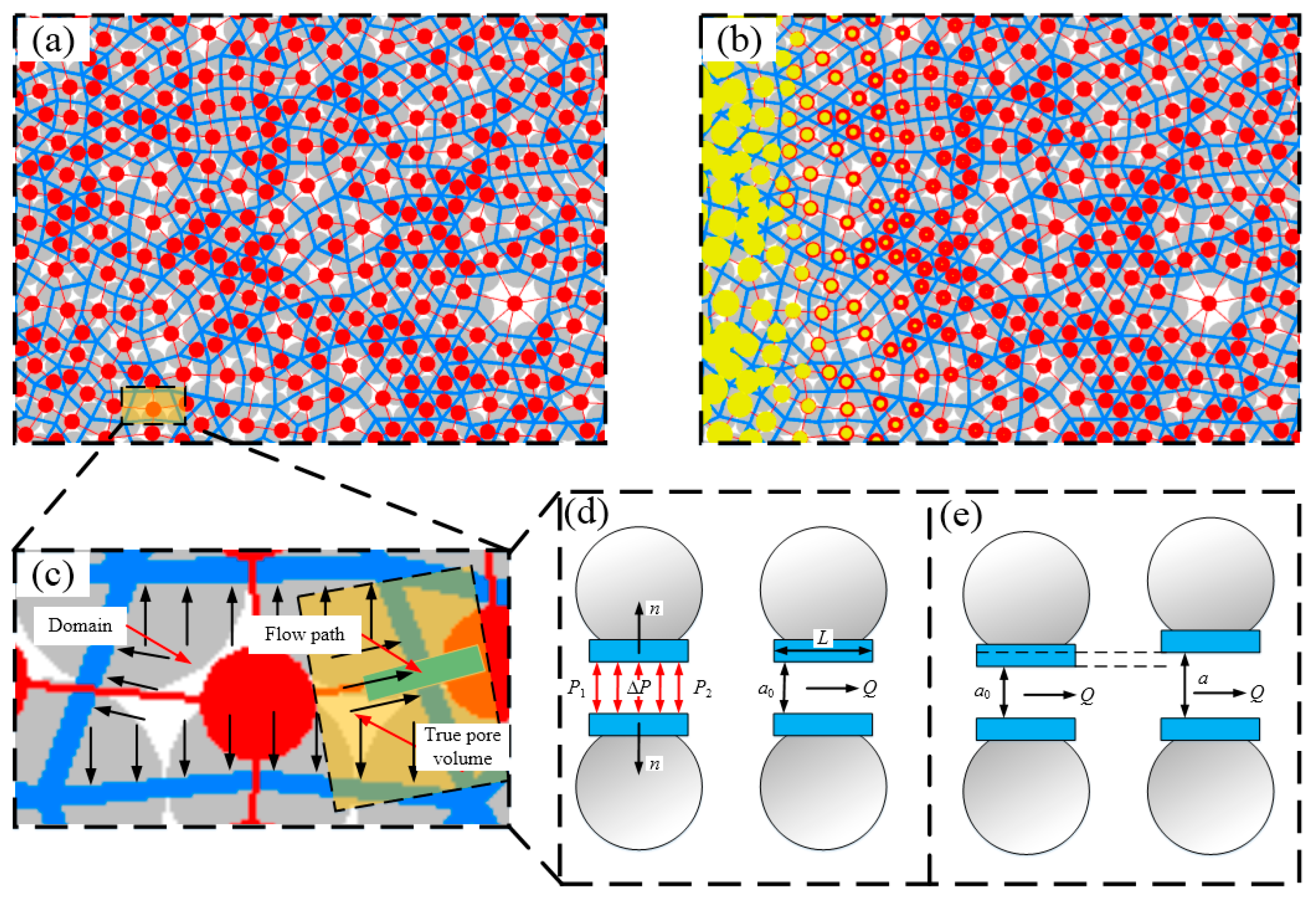
Figure 5.
Synthetic rock mass (SRM) method used in coupled hydro-mechanical simulation (a) fluid domains (blue polygons), centers of domains (red circles), and flow pipes (red lines) composing the fluid network; (b) distribution of fluid pressure; (c) domain and flow channel; (d) fluid pressure build up; (e) change of aperture.
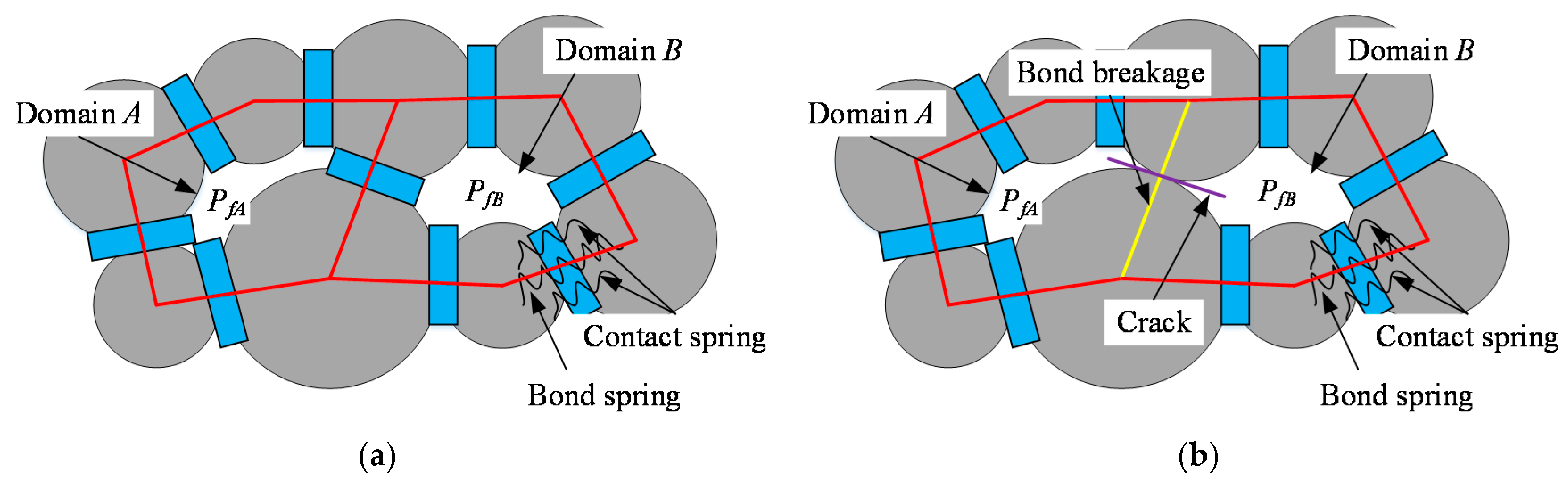
Figure 6.
Bond breakage and fluid pressure balancing according to Equation (23) in the two domains: (a) fluid pressure before a crack initiation and (b) fluid pressure after a crack initiation.
Figure 6.
Bond breakage and fluid pressure balancing according to Equation (23) in the two domains: (a) fluid pressure before a crack initiation and (b) fluid pressure after a crack initiation.
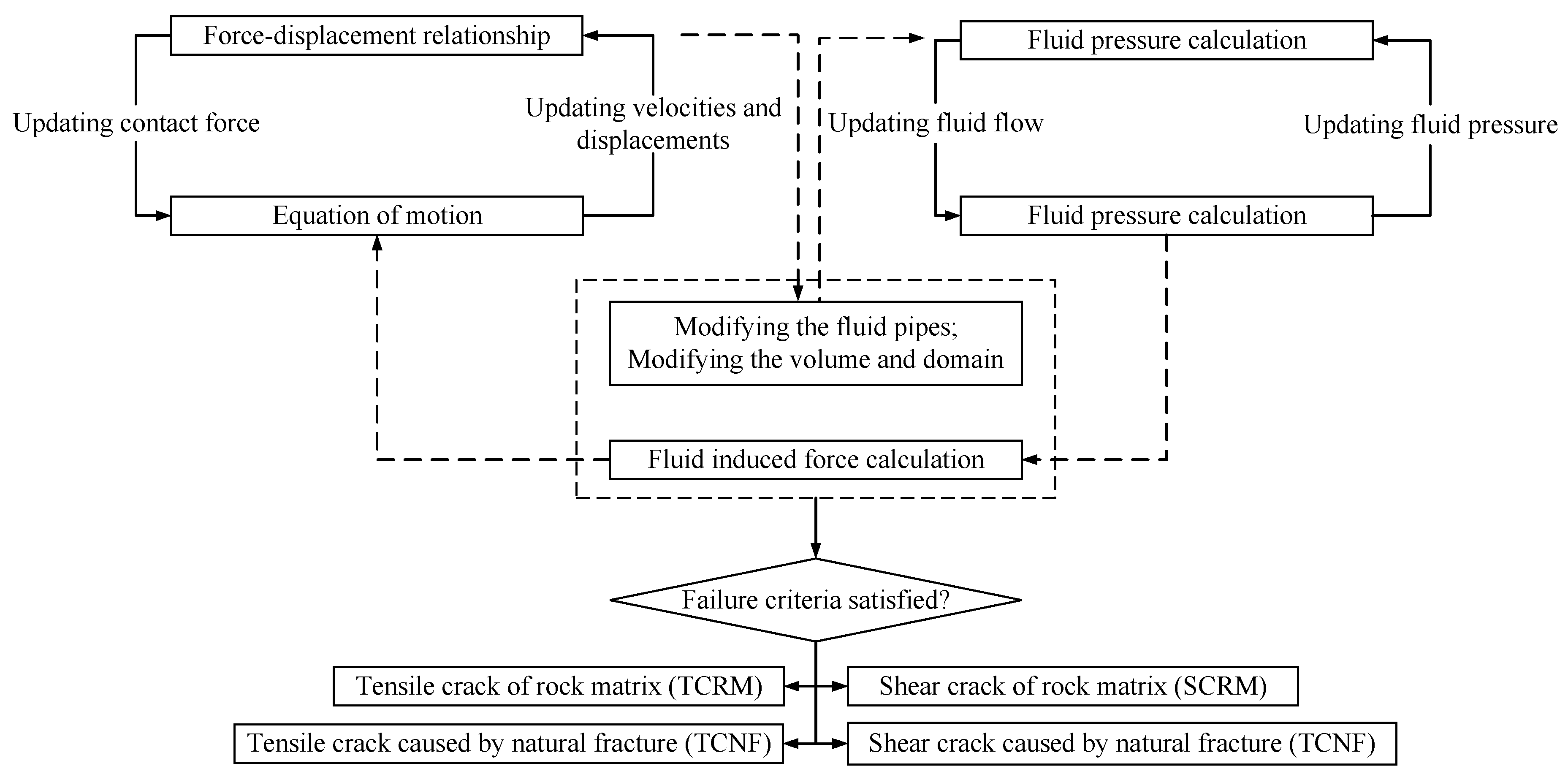
Figure 7.
Modeling procedures for a hydro-mechanical coupling.
Figure 7.
Modeling procedures for a hydro-mechanical coupling.
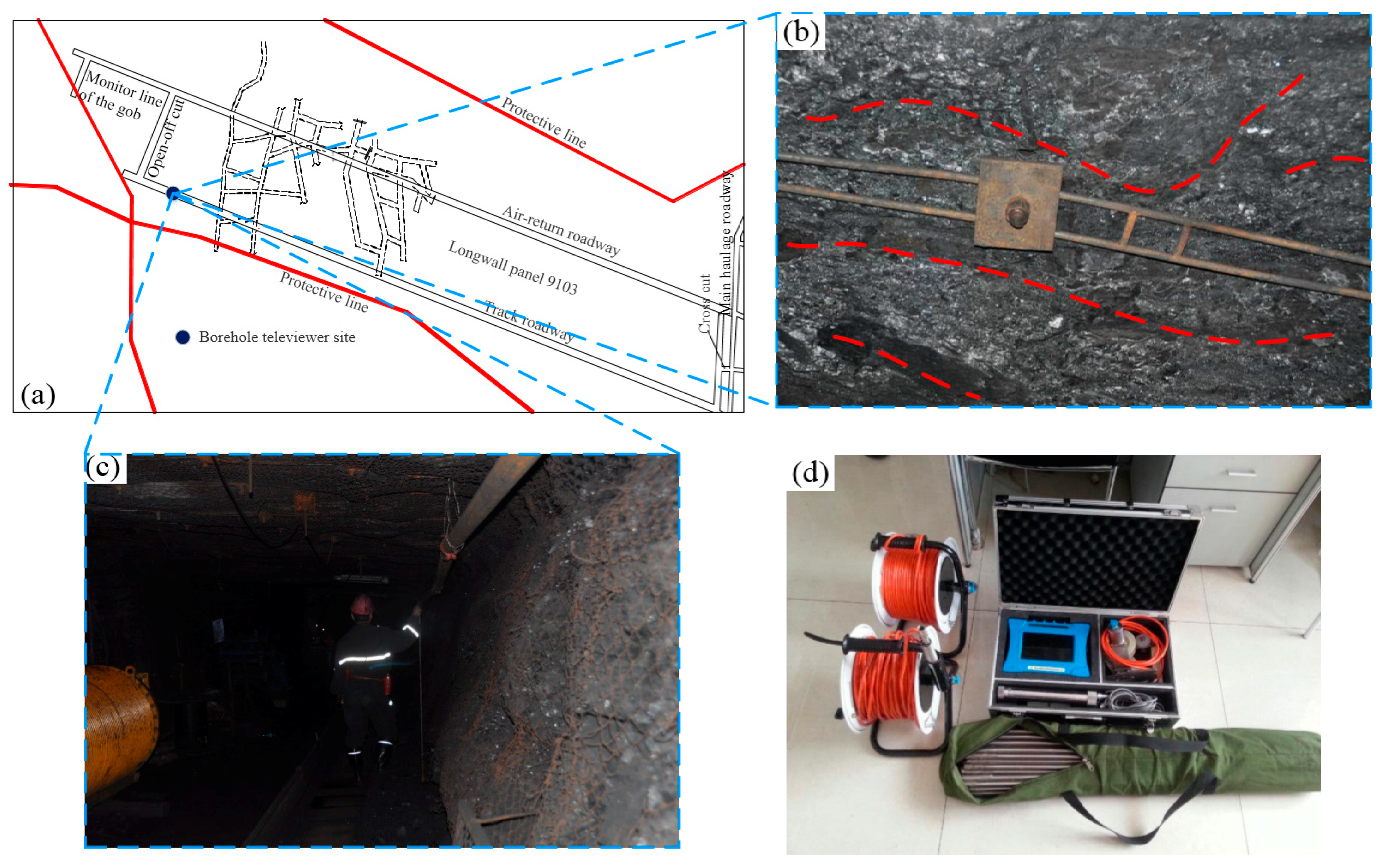
Figure 8.
(a) Plan view of the study site at Huahong coal mine, China; photographs of (b) roof (c) rib; (d) test equipment of borehole image.
Figure 8.
(a) Plan view of the study site at Huahong coal mine, China; photographs of (b) roof (c) rib; (d) test equipment of borehole image.
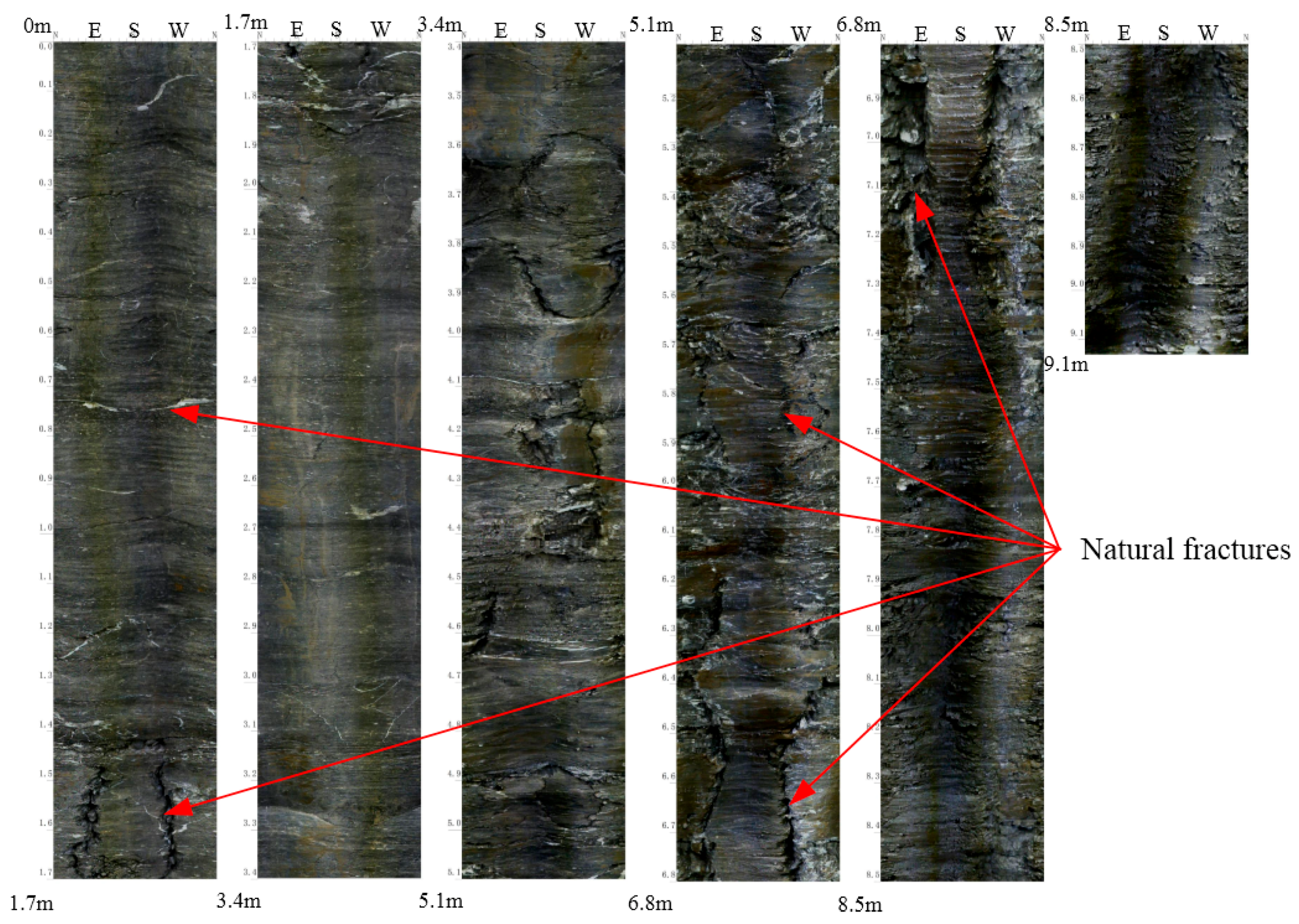
Figure 9.
Optical televiewer image of the borehole drilled vertically in the roof at the Huahong coal mine, China.
Figure 9.
Optical televiewer image of the borehole drilled vertically in the roof at the Huahong coal mine, China.
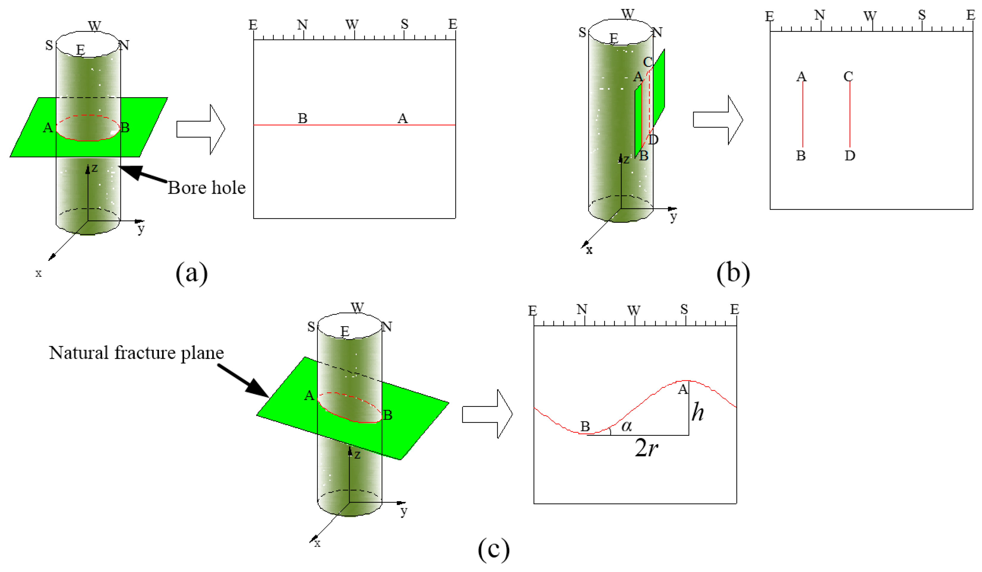
Figure 10.
The intersection of the drill hole and the structure surface: (a) vertical intersection; (b) parallel intersection and (c) inclined intersection.
Figure 10.
The intersection of the drill hole and the structure surface: (a) vertical intersection; (b) parallel intersection and (c) inclined intersection.
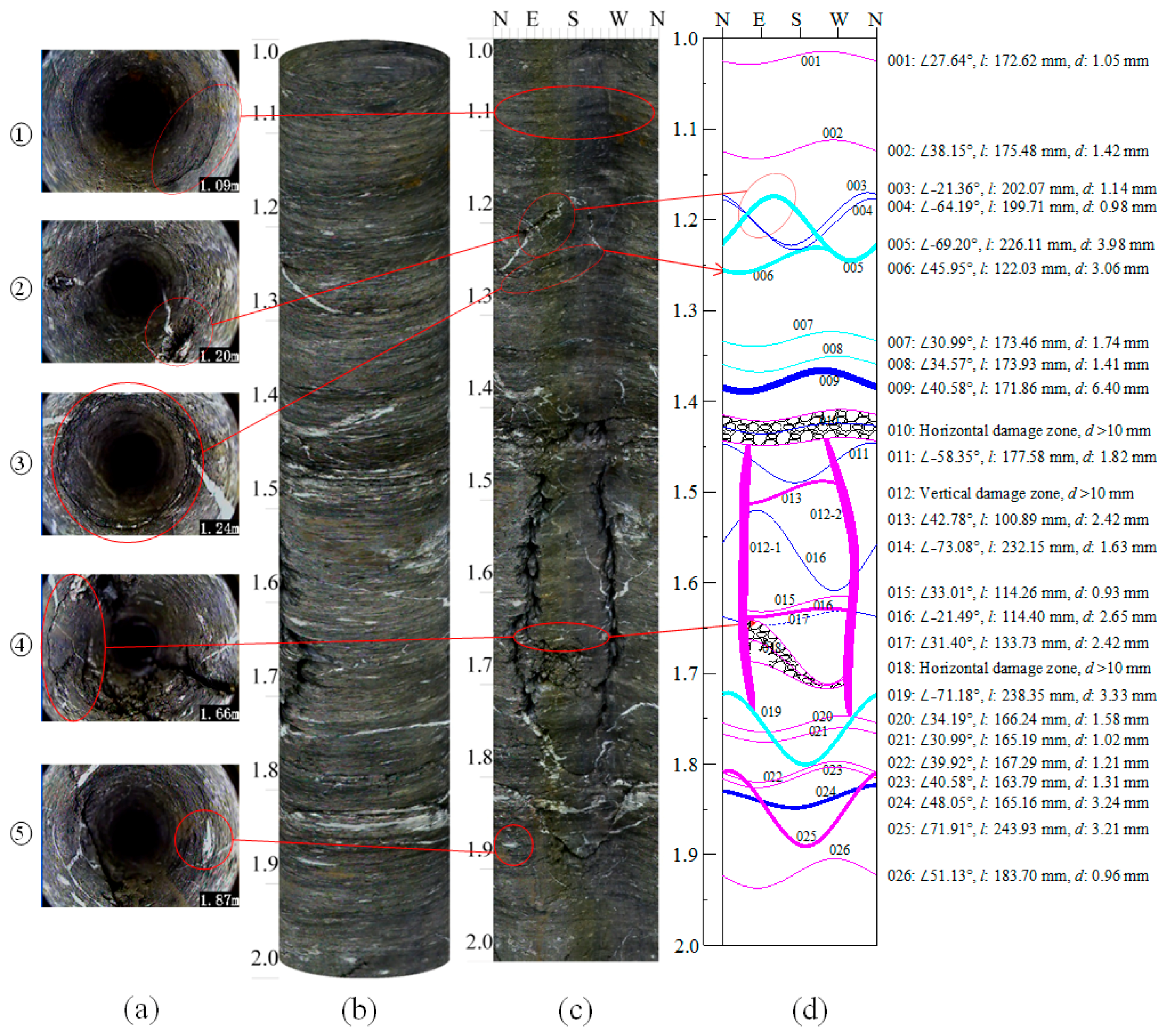
Figure 11.
(a) Typical point; (b) virtual map of borehole image in 3-D; (c) plan view of the drill hole; (d) measurements of natural fracture (NF).
Figure 11.
(a) Typical point; (b) virtual map of borehole image in 3-D; (c) plan view of the drill hole; (d) measurements of natural fracture (NF).
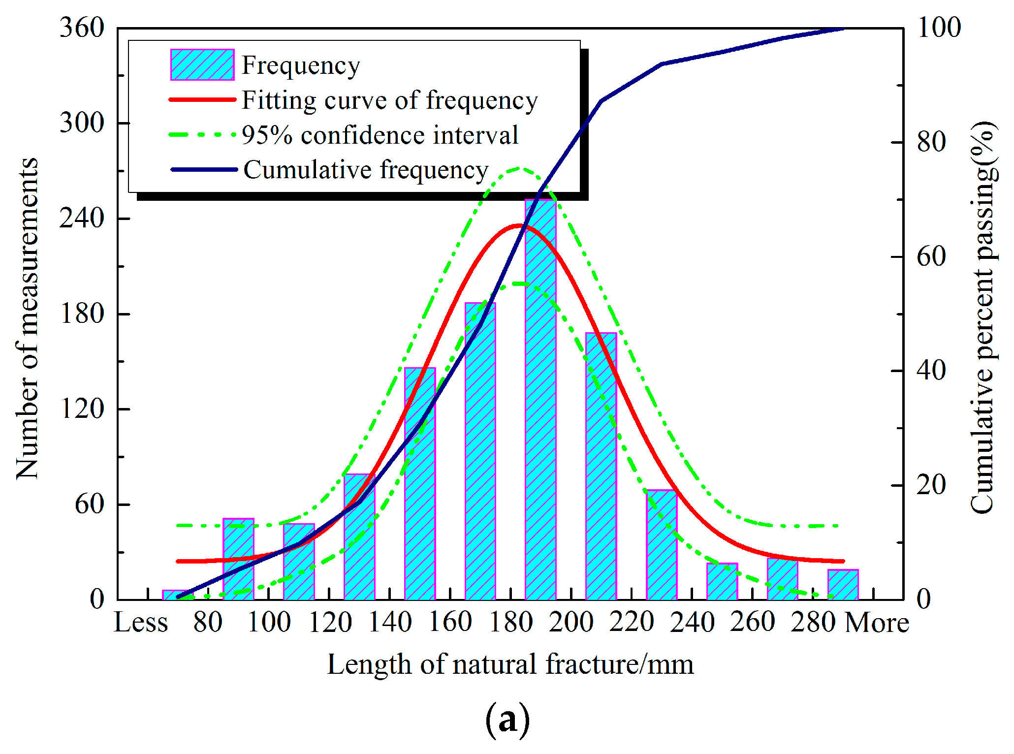
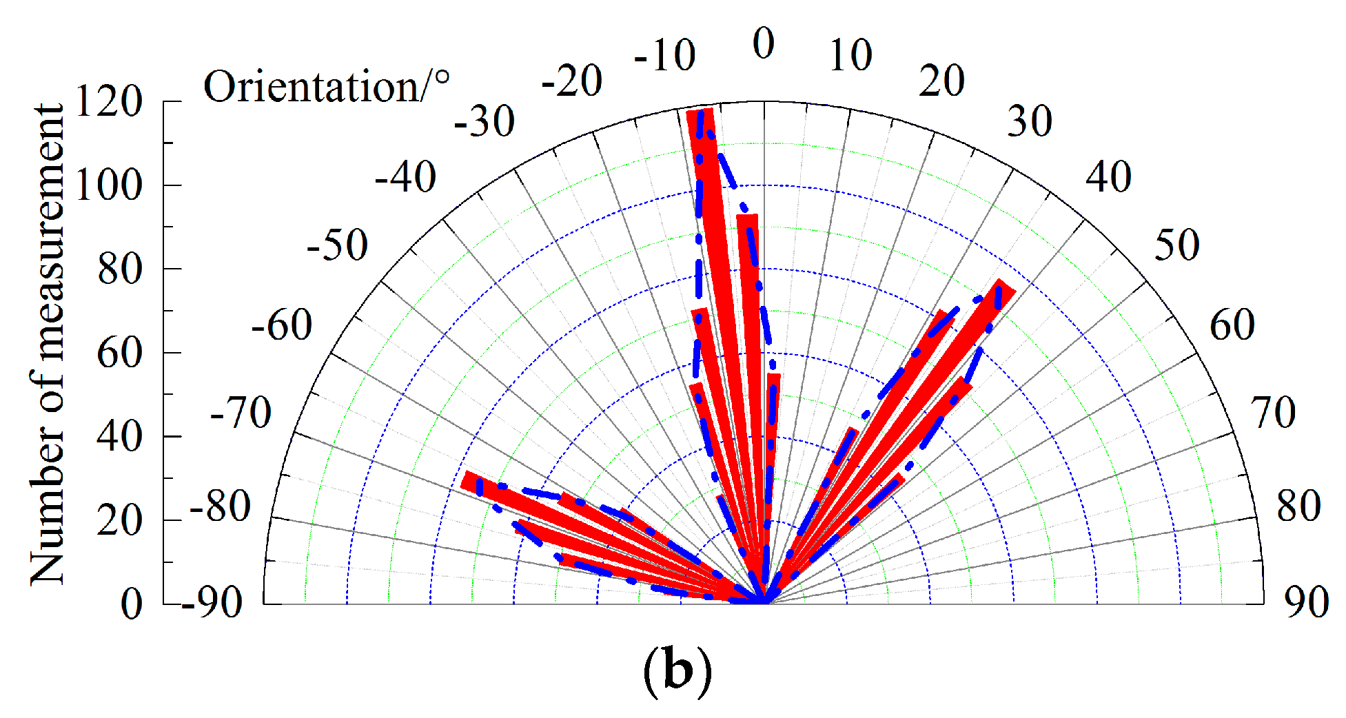
Figure 12.
Statistical results of natural fracture (NF) (a) length and (b) dip angle.
Figure 12.
Statistical results of natural fracture (NF) (a) length and (b) dip angle.
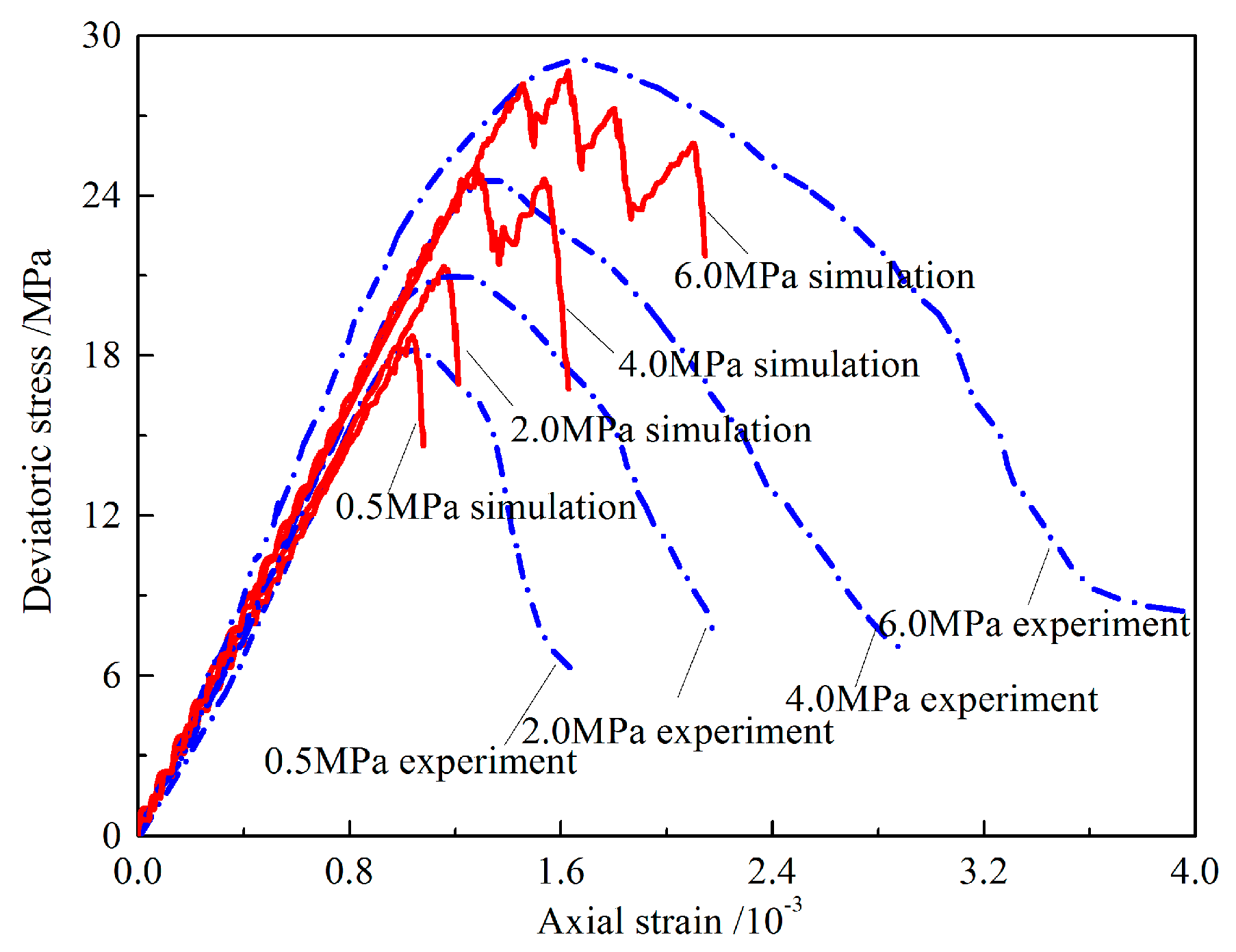
Figure 13.
Comparison between experimental and numerical deviation stress versus axial strain curves.
Figure 13.
Comparison between experimental and numerical deviation stress versus axial strain curves.
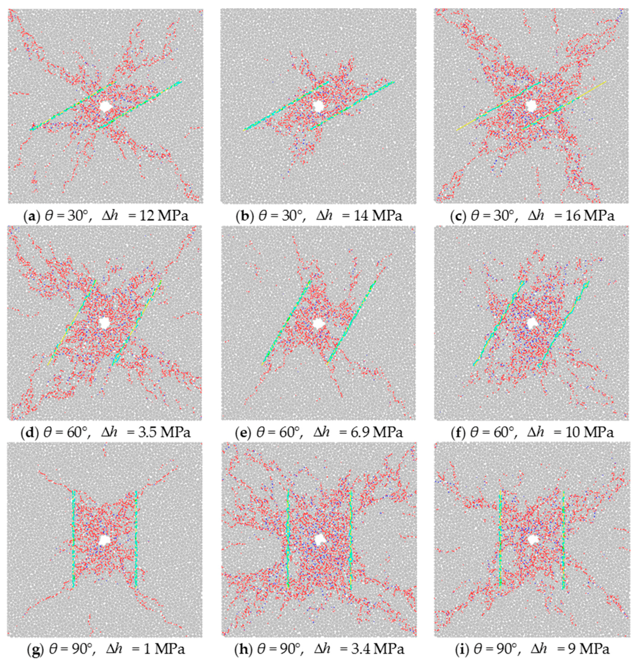
Figure 14.
Numerical results of HF and NF interactions at different values of θ and .
Figure 14.
Numerical results of HF and NF interactions at different values of θ and .
Figure 15.
Comparison between the interactive behavior in the physical experiment and numerical simulation.
Figure 15.
Comparison between the interactive behavior in the physical experiment and numerical simulation.
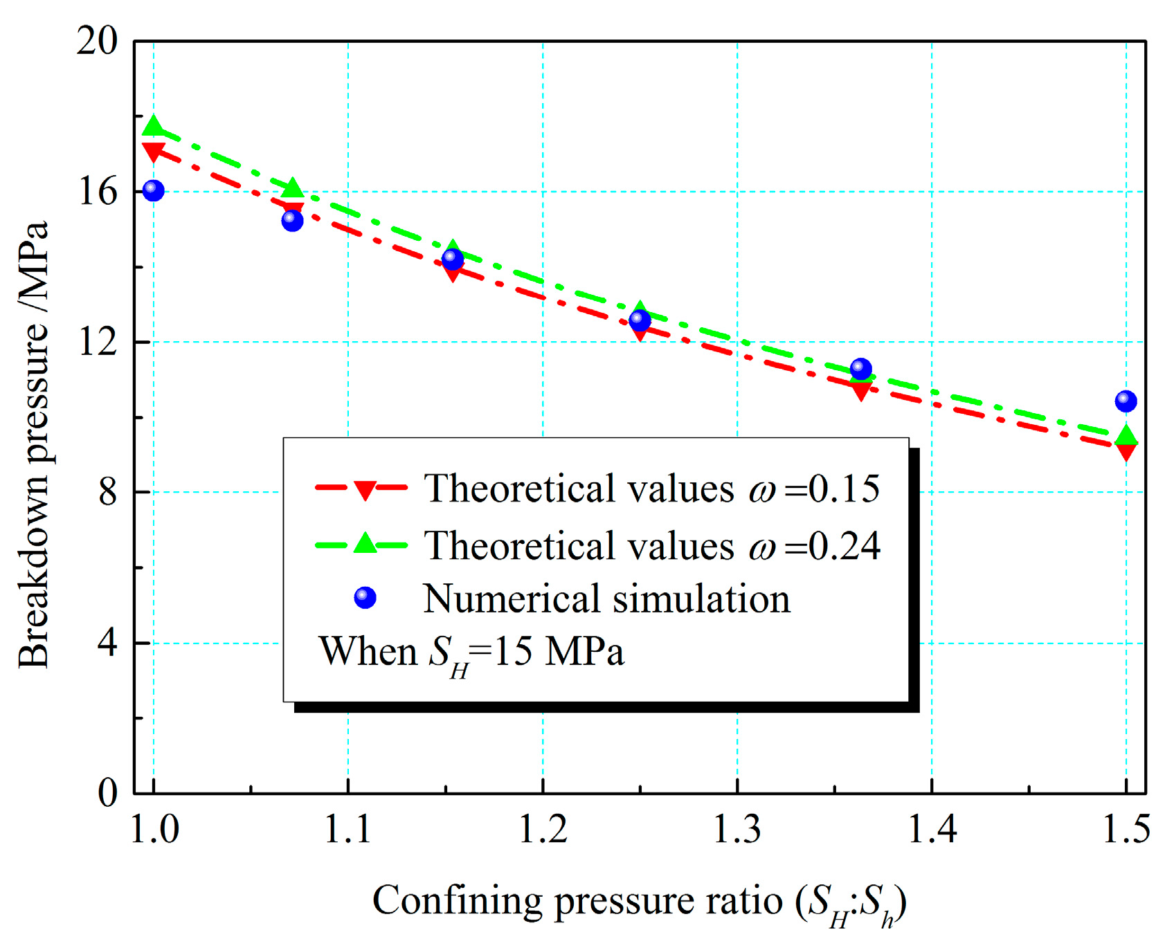
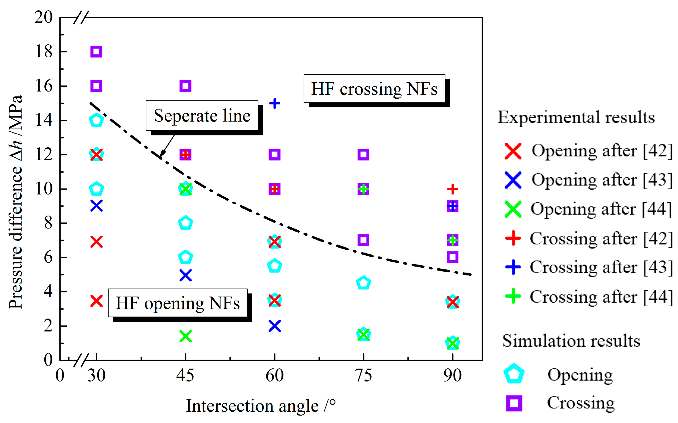
Figure 16.
Comparison of breakdown pressure under different confining pressure ratios obtained by the theoretical equation and numerical simulations.
Figure 16.
Comparison of breakdown pressure under different confining pressure ratios obtained by the theoretical equation and numerical simulations.
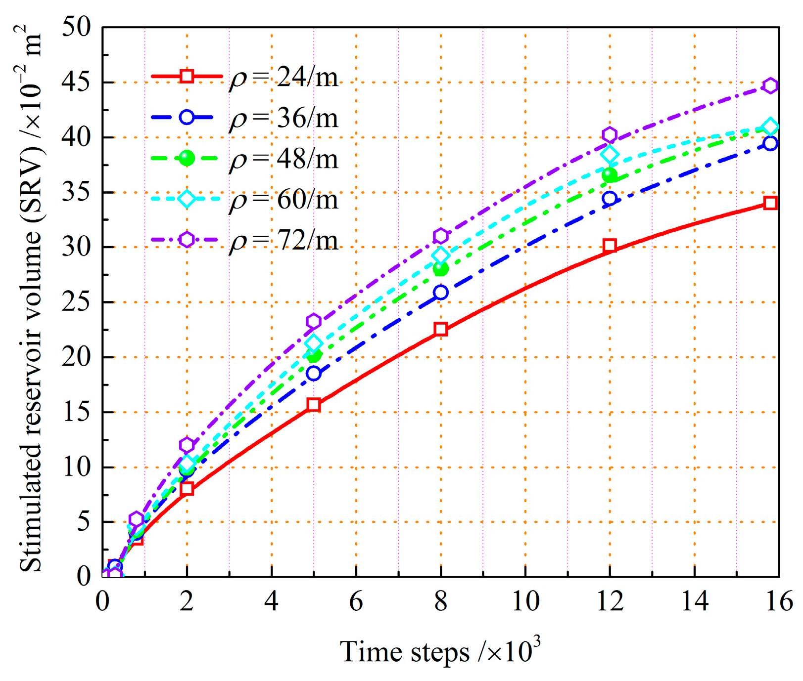
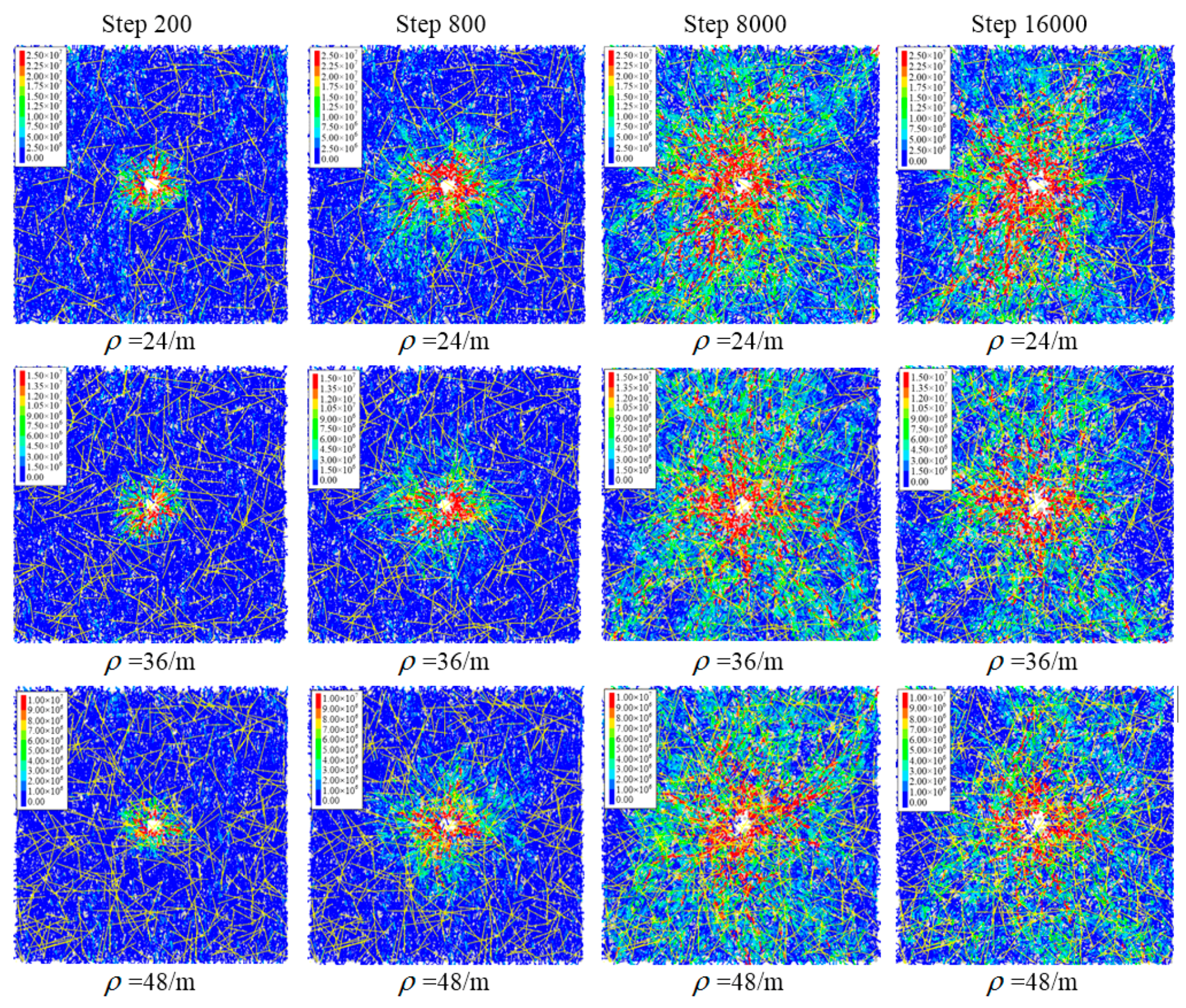
Figure 17.
Change of stimulated reservoir volume (SRV) with time steps when natural fracture (NF) density ranges from 24 to 72/m when injection rate is 2.0 × 10⁻⁶ m3/s and SH: Sh = 10:5.
Figure 17.
Change of stimulated reservoir volume (SRV) with time steps when natural fracture (NF) density ranges from 24 to 72/m when injection rate is 2.0 × 10⁻⁶ m3/s and SH: Sh = 10:5.
Figure 18.
Evolution process of injection pressure induced by NF densities of rock formations when injection rate is 2.0 × 10⁻⁶ m3/s and SH: Sh = 10:5.
Figure 18.
Evolution process of injection pressure induced by NF densities of rock formations when injection rate is 2.0 × 10⁻⁶ m3/s and SH: Sh = 10:5.
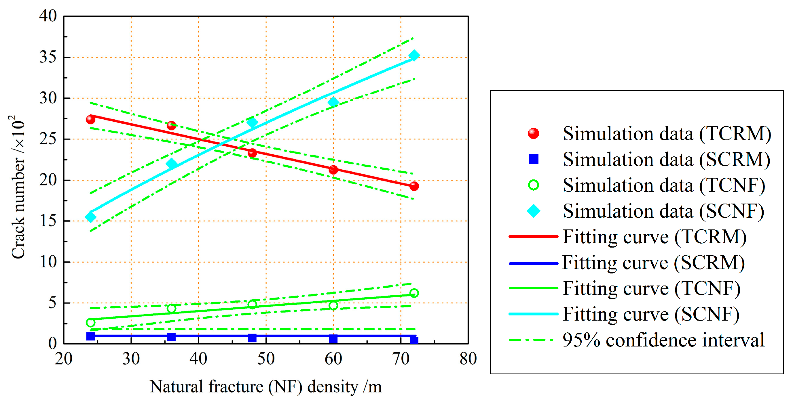
Figure 19.
Variation of tensile crack of rock matrix (TCRM), shear crack of rock matrix (SCRM), tensile crack of natural fracture (TCNF), and shear crack of rock matrix (SCNF) in various NF densities.
Figure 19.
Variation of tensile crack of rock matrix (TCRM), shear crack of rock matrix (SCRM), tensile crack of natural fracture (TCNF), and shear crack of rock matrix (SCNF) in various NF densities.
Figure 20.
Change of injection pressure with CPR when NF density ranges from 24/m to 72/m and injection rate is 2.0 × 10⁻⁶ m3/s.
Figure 20.
Change of injection pressure with CPR when NF density ranges from 24/m to 72/m and injection rate is 2.0 × 10⁻⁶ m3/s.
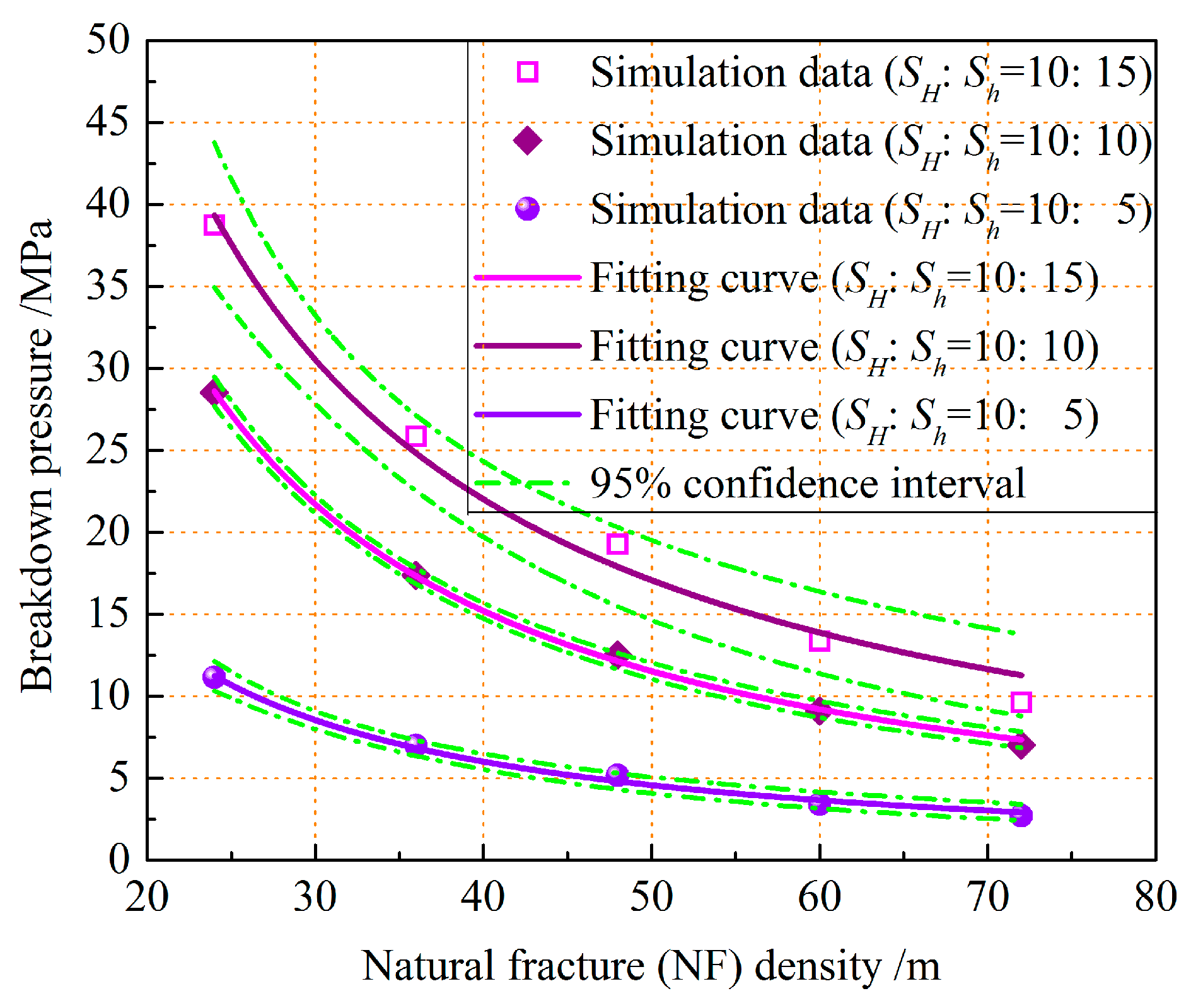
Figure 21.
Variation of breakdown pressure with NF density under different confining pressure ratios and injection rate is 2.0 × 10⁻⁶ m3/s.
Figure 21.
Variation of breakdown pressure with NF density under different confining pressure ratios and injection rate is 2.0 × 10⁻⁶ m3/s.
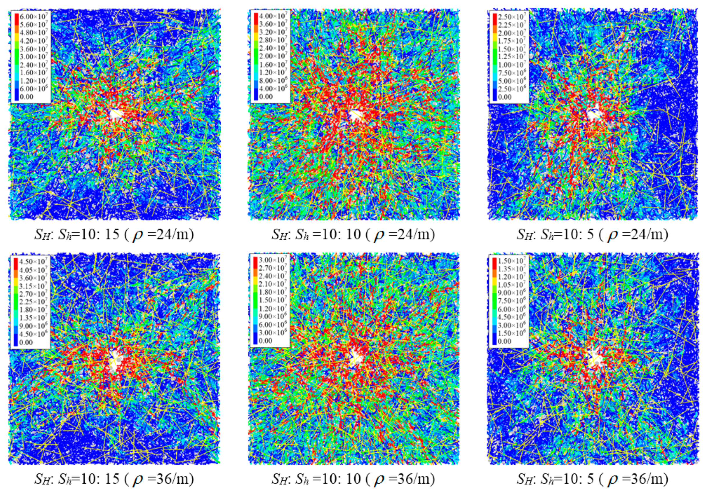
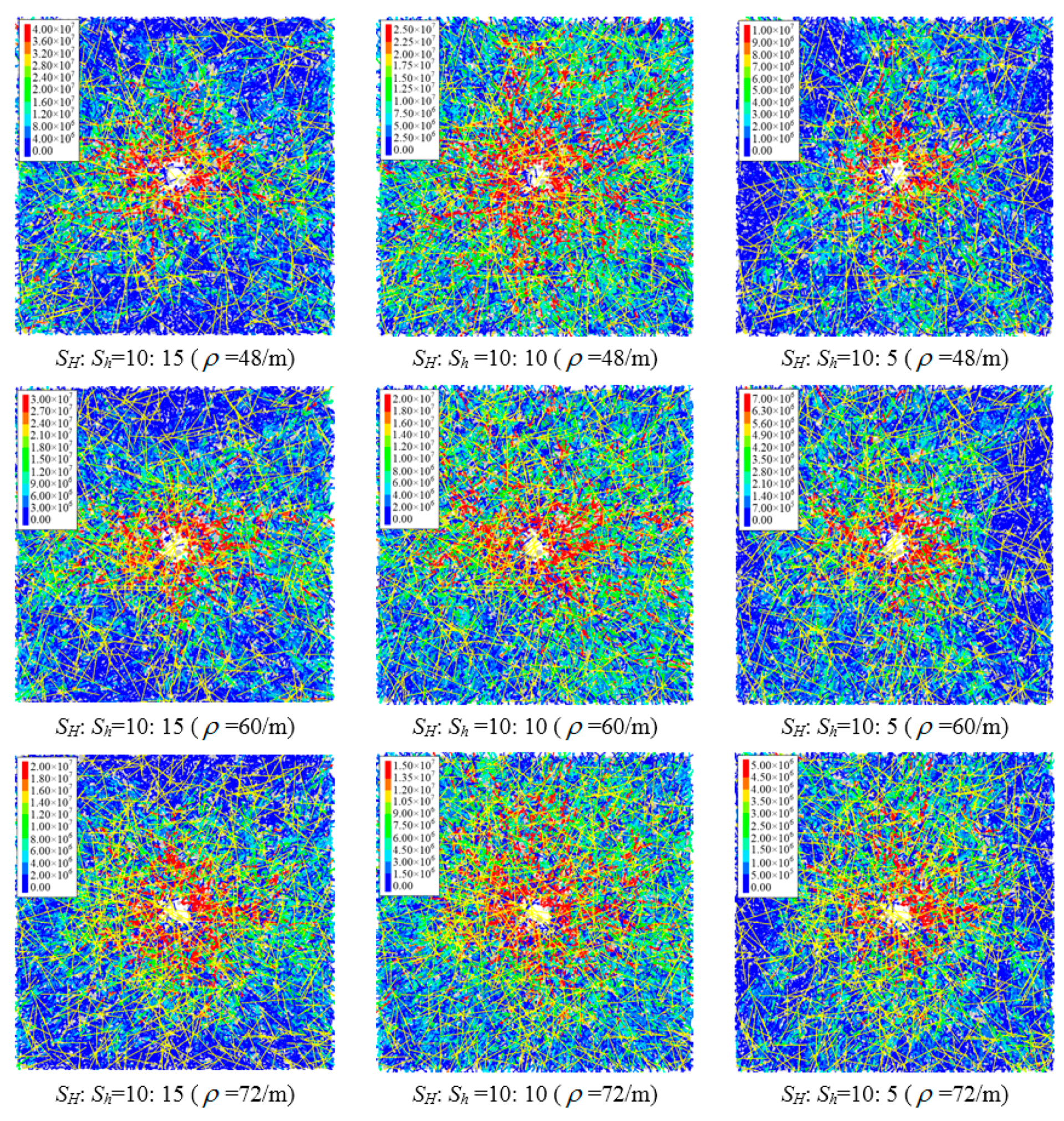
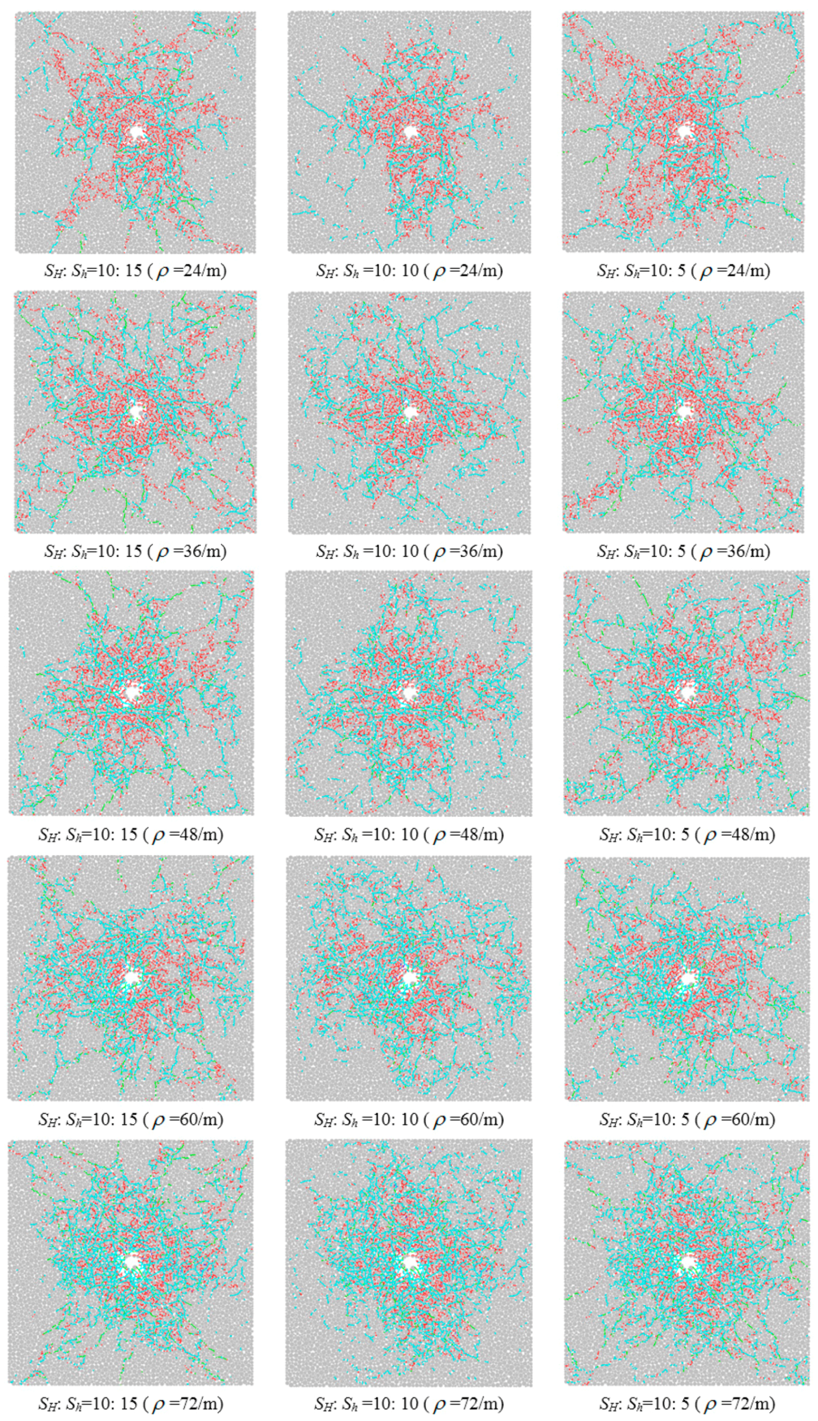
Figure 22.
Change of crack distribution with confining pressure ratio when NF density ranges from 24/m to 72/m and injection rate is 2.0 × 10⁻⁶ m3/s.
Figure 22.
Change of crack distribution with confining pressure ratio when NF density ranges from 24/m to 72/m and injection rate is 2.0 × 10⁻⁶ m3/s.
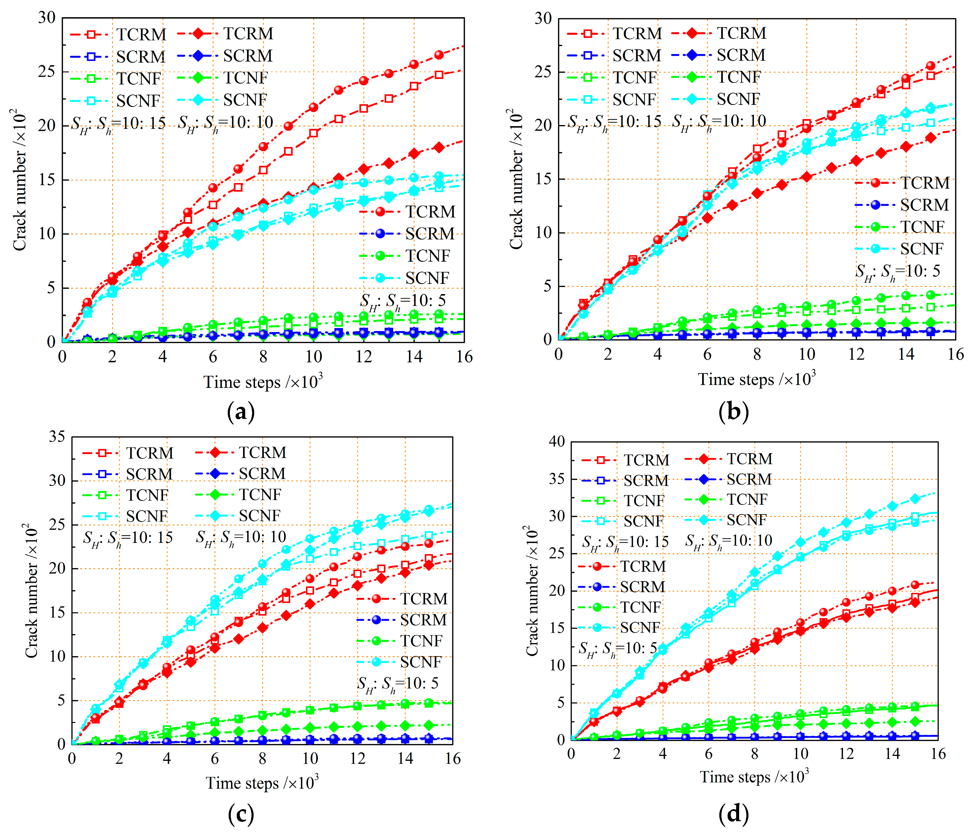
Figure 23.
Incremental accumulation of TCRM, SCRM, TCNF, and SCNF in various NF densities when injection rate is 2.0 × 10⁻⁶ m3/s; (a) = 24/m; (b) = 36/m; (c) = 48/m; (d) = 60/m; and (e) = 72/m.
Figure 23.
Incremental accumulation of TCRM, SCRM, TCNF, and SCNF in various NF densities when injection rate is 2.0 × 10⁻⁶ m3/s; (a) = 24/m; (b) = 36/m; (c) = 48/m; (d) = 60/m; and (e) = 72/m.
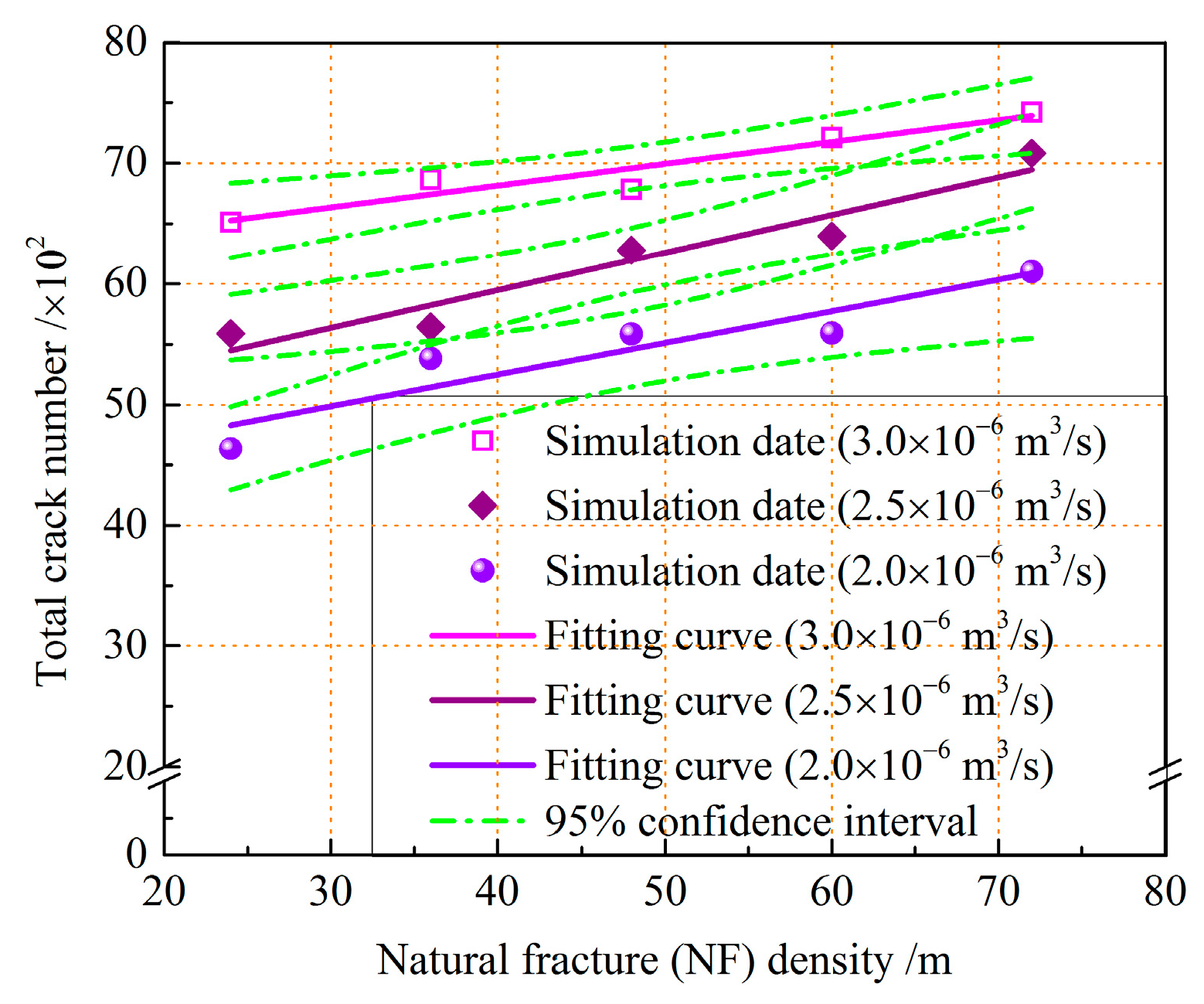
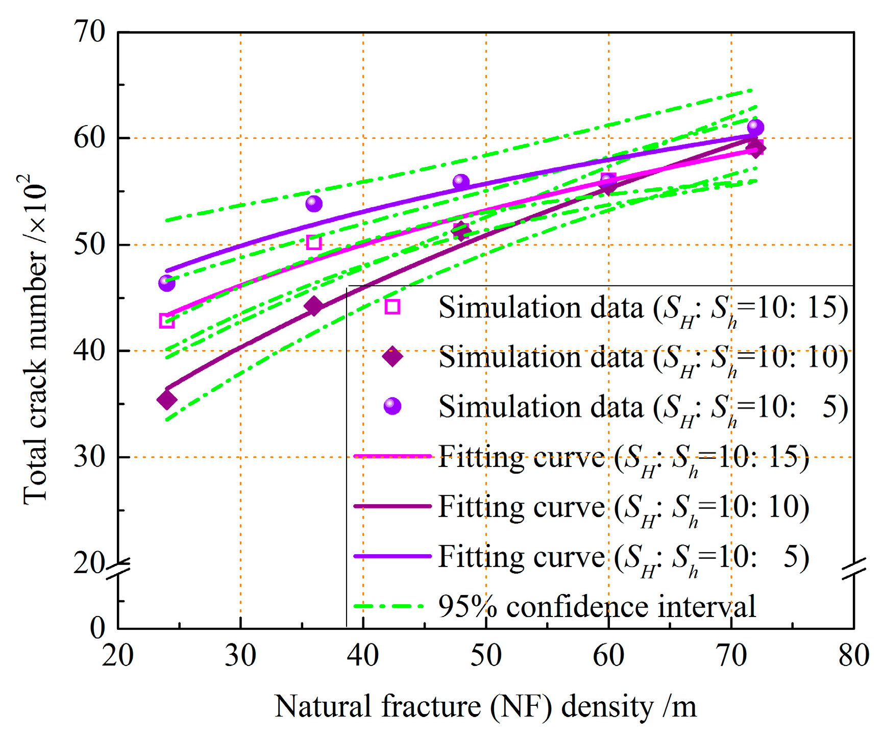
Figure 24.
Variation of total number of cracks with NF density under different confining pressure ratios and injection rate is 2.0 × 10⁻⁶ m3/s.
Figure 24.
Variation of total number of cracks with NF density under different confining pressure ratios and injection rate is 2.0 × 10⁻⁶ m3/s.
Figure 25.
Change of injection pressure with injection rate when NF density ranges from 24/m to 72/m and SH: Sh = 10:5.
Figure 25.
Change of injection pressure with injection rate when NF density ranges from 24/m to 72/m and SH: Sh = 10:5.
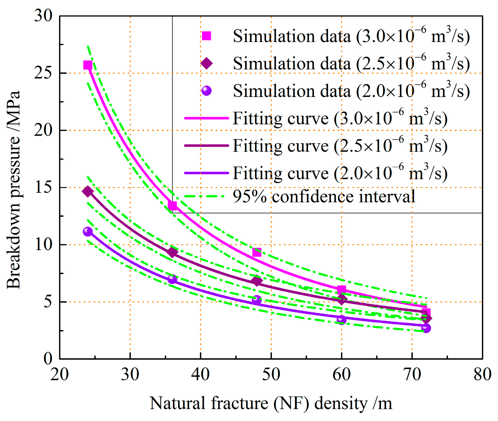
Figure 26.
Variation of breakdown pressure with NF density under different injection rates and confining pressure ratio is SH: Sh = 10:5.
Figure 26.
Variation of breakdown pressure with NF density under different injection rates and confining pressure ratio is SH: Sh = 10:5.
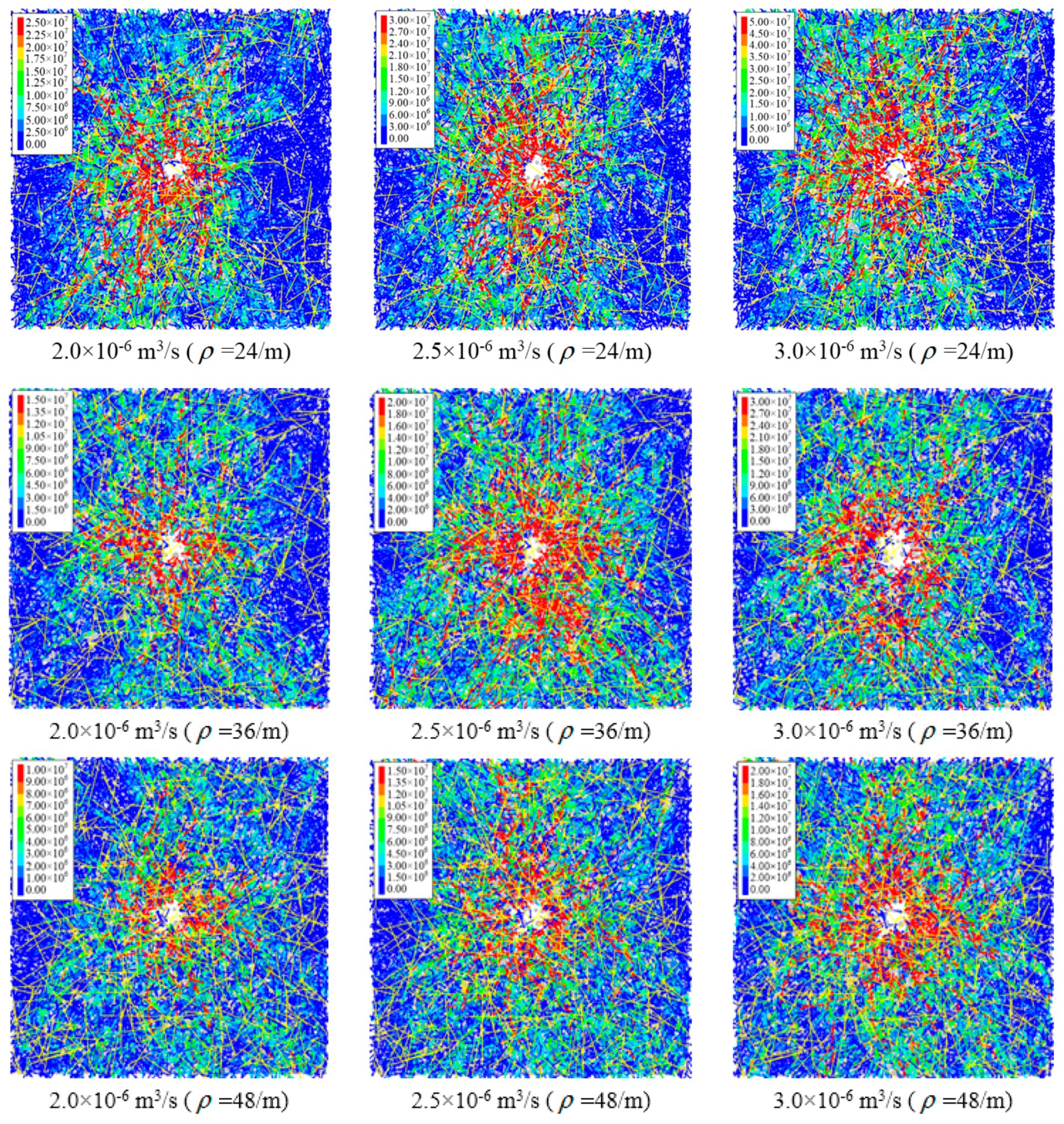
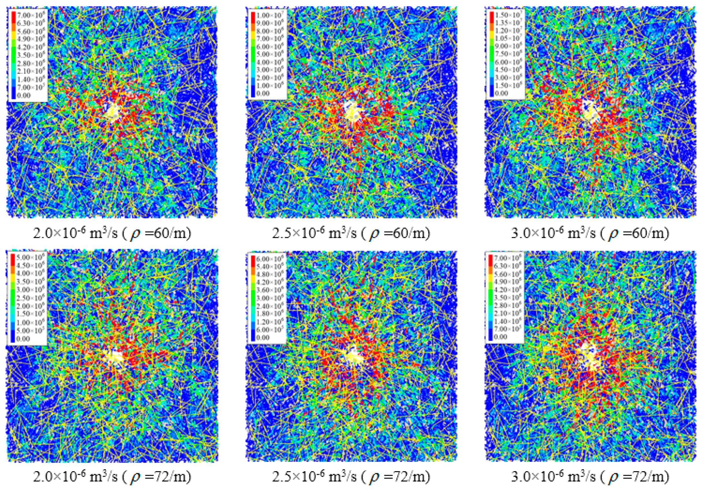
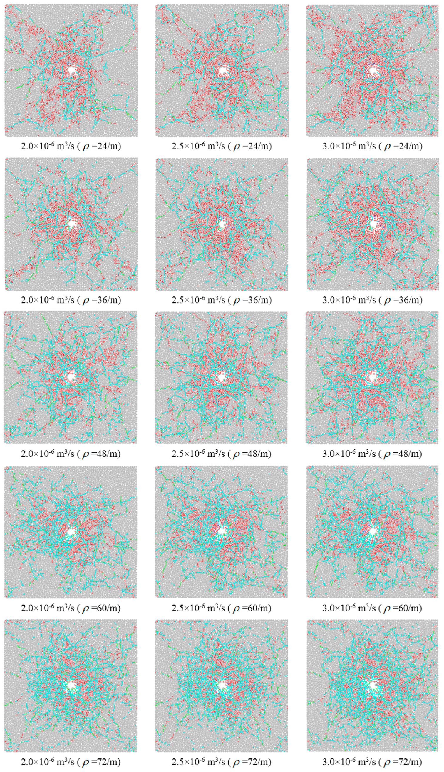
Figure 27.
Change of crack distribution with injection rate when NF density ranges from 24/m to 72/m and confining pressure ratio is SH: Sh = 10:5.
Figure 27.
Change of crack distribution with injection rate when NF density ranges from 24/m to 72/m and confining pressure ratio is SH: Sh = 10:5.
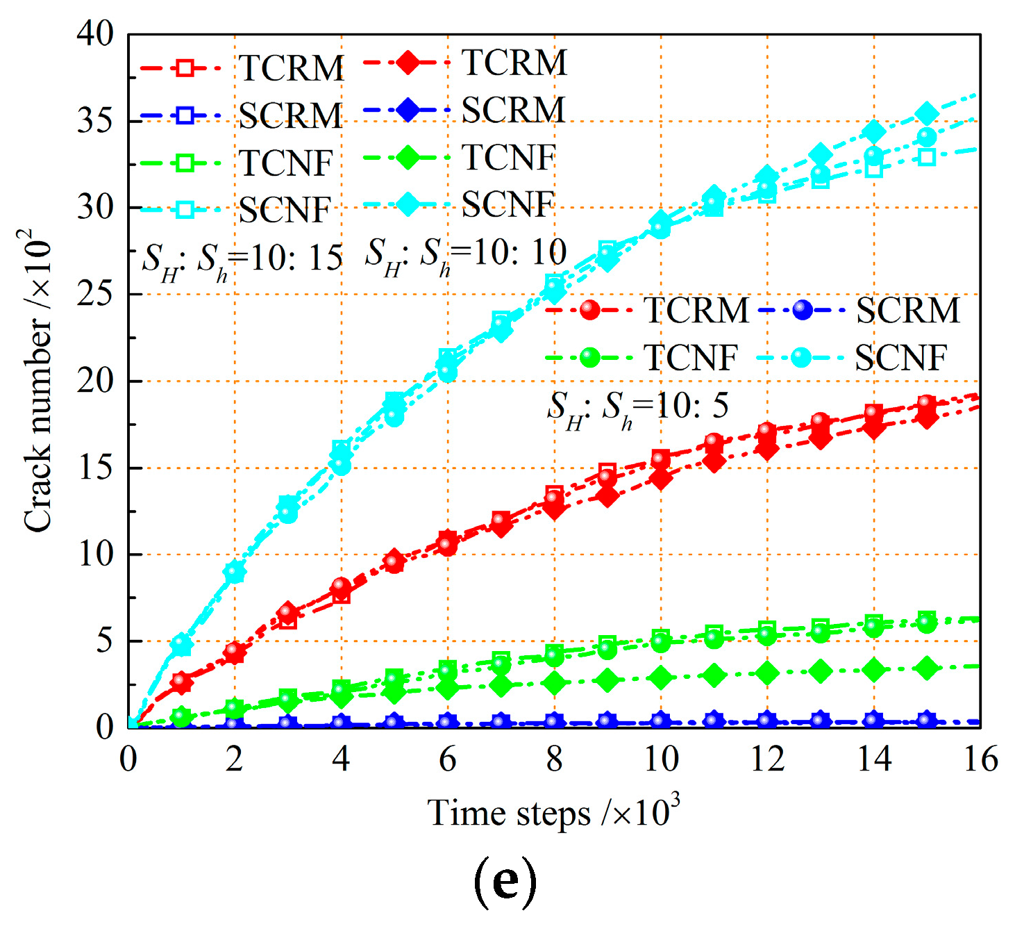
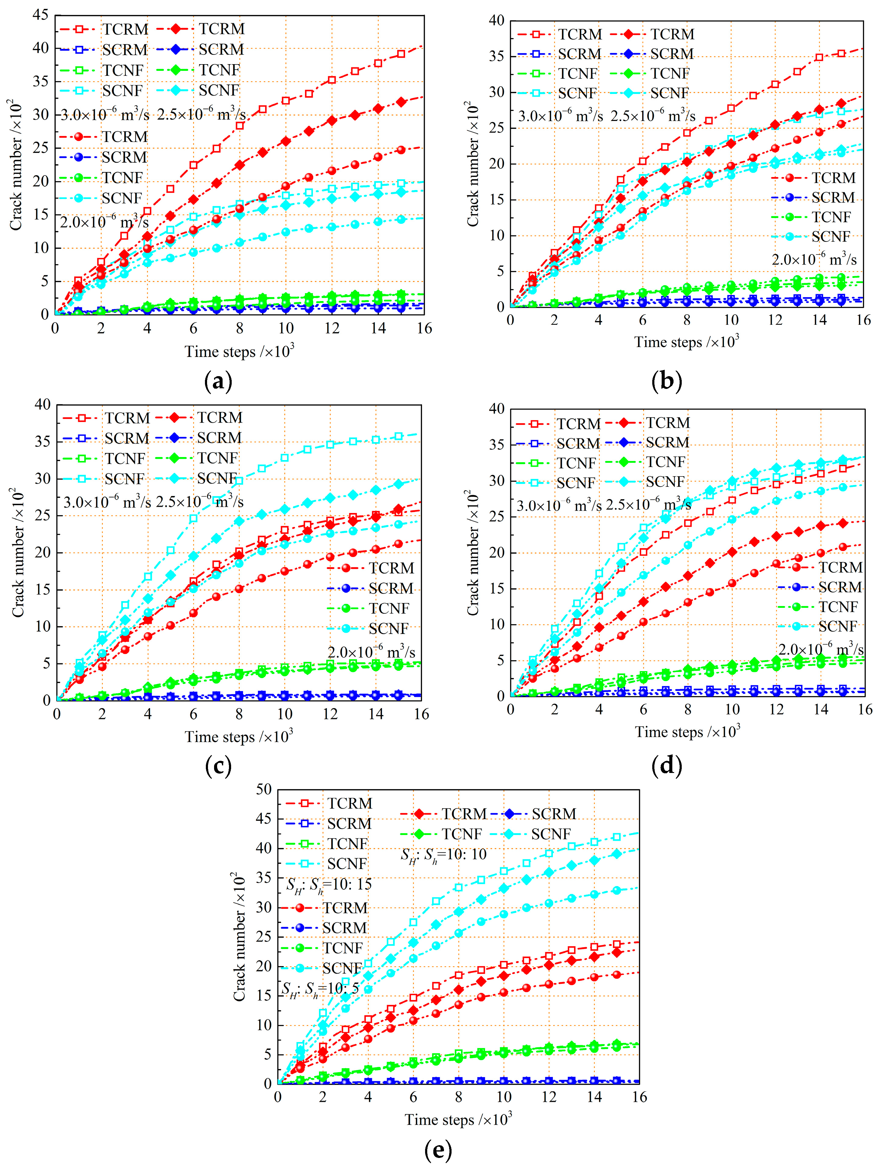
Figure 28.
Incremental accumulation of TCRM, SCRM, TCNF, and SCNF in various NF densities when the confining pressure ratio is SH: Sh = 10:5; (a) = 24/m; (b) = 36/m; (c) = 48/m; (d) = 60/m; and (e) = 72/m.
Figure 28.
Incremental accumulation of TCRM, SCRM, TCNF, and SCNF in various NF densities when the confining pressure ratio is SH: Sh = 10:5; (a) = 24/m; (b) = 36/m; (c) = 48/m; (d) = 60/m; and (e) = 72/m.
Figure 29.
Variation of the total number of cracks with NF density under different injection rates and confining pressure ratio is SH: Sh = 10:5.
Figure 29.
Variation of the total number of cracks with NF density under different injection rates and confining pressure ratio is SH: Sh = 10:5.
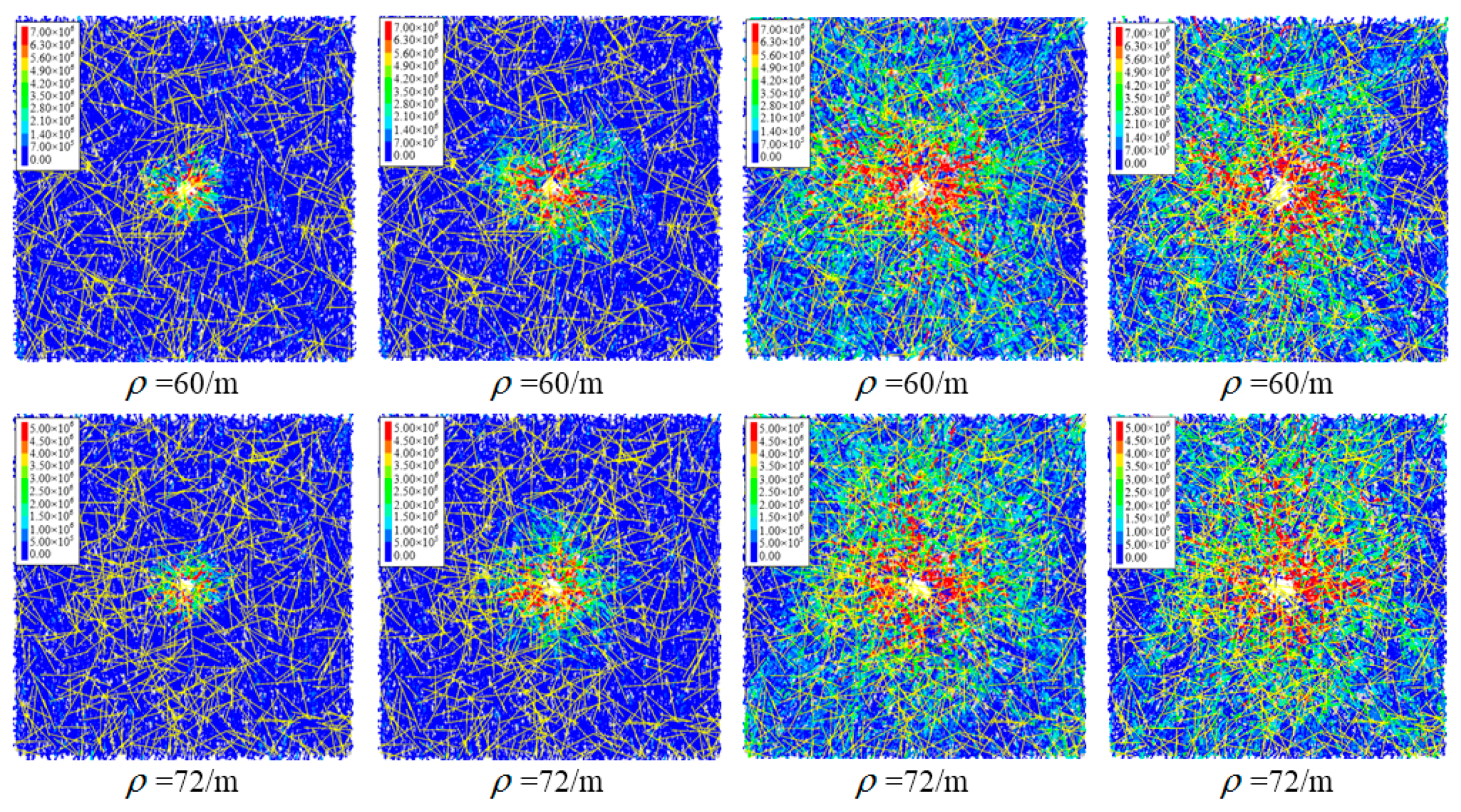
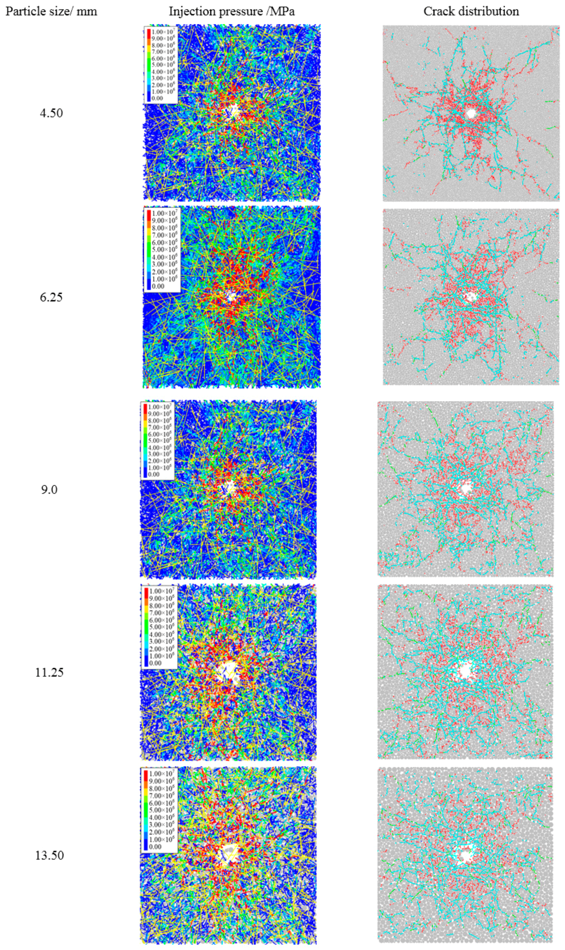
Figure 30.
Change of injection pressure and crack distribution with particle size when NF density is 48/m and SH: Sh = 10:5.
Figure 30.
Change of injection pressure and crack distribution with particle size when NF density is 48/m and SH: Sh = 10:5.
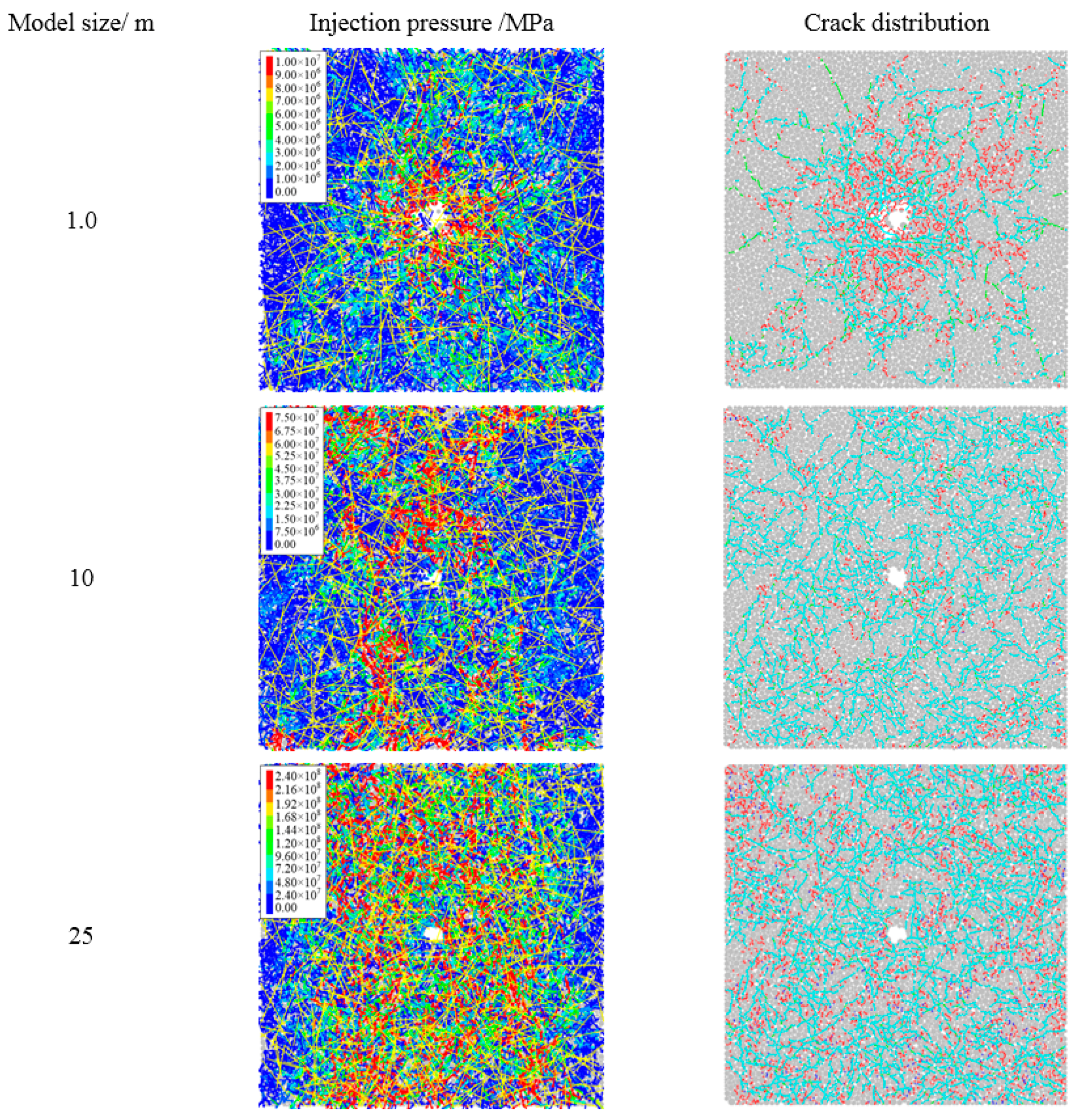
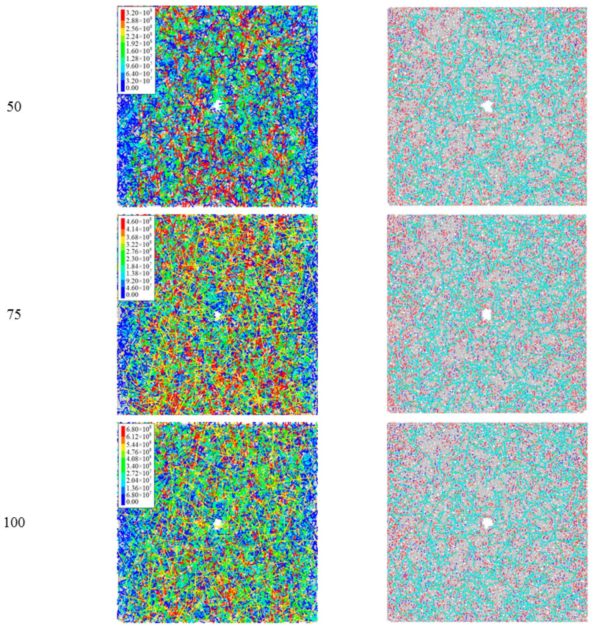
Figure 31.
Change in injection pressure and crack distribution with model size when NF density is 48/m and SH: Sh = 10:5.
Figure 31.
Change in injection pressure and crack distribution with model size when NF density is 48/m and SH: Sh = 10:5.
Table 1.
Micro-properties used in intact rock for simulated specimens after calibration [
41].
Table 1.
Micro-properties used in intact rock for simulated specimens after calibration [
41].
| Micro-Parameters | Unit | Values |
|---|
| The minimum particle radius (Rmin) | mm | 1.0 |
| Ratio of maximum and minimum particle radius (Rmax/Rmin) | - | 1.67 |
| Particle density (ρp) | kg/m3 | 2800 |
| Particle friction coefficient (μ) | - | 0.55 |
| Young’s modulus of the particle (E) | GPa | 14.4 |
| Parallel-bond radius multiplier (λ) | - | 1.0 |
| Young’s modulus of the parallel bond () | GPa | 14.4 |
| Normal stiffness of the parallel bond (mean) | MPa | 14.7 |
| Normal stiffness of the parallel bond (std deviation) | MPa | 3.6 |
| Shear stiffness of the parallel bond (mean) | MPa | 9.2 |
| Shear stiffness of the parallel bond (std deviation) | MPa | 2.4 |
Table 2.
Micro-properties used in smooth joint (SJ) contact for simulated specimens after calibration.
Table 2.
Micro-properties used in smooth joint (SJ) contact for simulated specimens after calibration.
| Parameters | Unit | Values |
|---|
| Smooth joint model | Normal stiffness () | GPa/m | 20.5 |
| Shear stiffness () | GPa/m | 18.5 |
| Tensile strength | MPa | 1.5 |
| Cohesion | MPa | 1.5 |
| Friction angle | ° | 0 |
Table 3.
Computational parameters of fluid properties.
Table 3.
Computational parameters of fluid properties.
| Fluid Parameters | Unit | Values |
|---|
| Injection rate | m3·s−1 | 2.0 × 10⁻⁶ |
| Fluid bulk modulus () | GPa | 2.0 |
| Fluid dynamic viscosity () | Pa·s | 1.1 × 10⁻⁴ |
| Initial fluid aperture () | m | 2.7 × 10⁻⁵ |
| Infinite fluid aperture () | m | 2.7 × 10⁻⁶ |
Table 4.
Fitting curve equations of the number of cracks for different NF densities.
Table 4.
Fitting curve equations of the number of cracks for different NF densities.
| Confining Pressure Ratios | Fitting Curve Equations | R-Squared |
|---|
| Tensile crack of rock matrix (TCRM) | | 0.96 |
| Shear crack of rock matrix (SCRM) | | 0.98 |
| Tensile crack caused by natural fracture (TCNF) | | 0.81 |
| Shear crack caused by natural fracture (SCNF) | | 0.92 |
Table 5.
Fitting curve equations of beakdown pressure under different confining pressure ratios.
Table 5.
Fitting curve equations of beakdown pressure under different confining pressure ratios.
| Confining Pressure Ratios | Fitting Curve Equations | R-Squared |
|---|
| SH: Sh = 10:15 | | 0.98 |
| SH: Sh = 10:10 | | 0.99 |
| SH: Sh = 10:5 | | 0.99 |
Table 6.
Fitting curve equations of total number of cracks under different confining pressure ratios.
Table 6.
Fitting curve equations of total number of cracks under different confining pressure ratios.
| Confining Pressure Ratios | Fitting Curve Equations | R-Squared |
|---|
| SH: Sh = 10:15 | | 0.96 |
| SH: Sh = 10:10 | | 0.98 |
| SH: Sh = 10:5 | | 0.88 |
Table 7.
Fitting curve equations of breakdown pressure under different injection rates.
Table 7.
Fitting curve equations of breakdown pressure under different injection rates.
| Injection Rates/m3·s−1 | Fitting Curve Equations | R-Squared |
|---|
| 2.0 × 10⁻⁶ | | 0.99 |
| 2.5 × 10⁻⁶ | | 0.98 |
| 3.0 × 10⁻⁶ | | 0.98 |
Table 8.
Fitting curve equations of the total number of cracks under different injection rates.
Table 8.
Fitting curve equations of the total number of cracks under different injection rates.
| Injection Rates/m3·s−1 | Fitting Curve Equations | R-Squared |
|---|
| 2.0 × 10⁻⁶ | | 0.87 |
| 2.5 × 10⁻⁶ | | 0.91 |
| 3.0 × 10⁻⁶ | | 0.83 |


