Article

Flexible Multi-Objective Transmission Expansion Planning with Adjustable Risk Aversion

1
Energy Flagship, The Commonwealth Scientific and Industrial Research Organization (CSIRO), Mayfield West, NSW 2304, Australia
2
School of Science and Engineering, Chinese University of Hong Kong (Shenzhen), Shenzhen 518172, China
3
Center for Intelligent Electricity Networks, The University of Newcastle, Callaghan, NSW 2308, Australia
*
Author to whom correspondence should be addressed.
Energies 2017, 10(7), 1036; https://doi.org/10.3390/en10071036
Submission received: 8 May 2017 / Revised: 27 June 2017 / Accepted: 13 July 2017 / Published: 20 July 2017
(This article belongs to the Section F: Electrical Engineering)

Abstract

:
This paper presents a multi-objective transmission expansion planning (TEP) framework. Rather than using the conventional deterministic reliability criterion, a risk component based on the probabilistic reliability criterion is incorporated into the TEP objectives. This risk component can capture the stochastic nature of power systems, such as load and wind power output variations, component availability, and incentive-based demand response (IBDR) costs. Specifically, the formulation of risk value after risk aversion is explicitly given, and it aims to provide network planners with the flexibility to conduct risk analysis. Thus, a final expansion plan can be selected according to individual risk preferences. Moreover, the economic value of IBDR is modeled and integrated into the cost objective. In addition, a relatively new multi-objective evolutionary algorithm called the MOEA/D is introduced and employed to find Pareto optimal solutions, and tradeoffs between overall cost and risk are provided. The proposed approach is numerically verified on the Garver’s six-bus, IEEE 24-bus RTS and Polish 2383-bus systems. Case study results demonstrate that the proposed approach can effectively reduce cost and hedge risk in relation to increasing wind power integration.

1. Introduction

Due to growing concern on climate change and energy sustainability, as one of the renewable resources, wind power is considered a promising alternative to conventional fossil-fuel power generators [1,2]. However, a major difficulty in the effective utilization of wind is its geographic dispersion and intermittency [3,4]. Specifically, wind resources are often abundant in remote areas, where transmission networks might be weak and bottlenecks exist [5]. Hence, transmission reinforcement may be required in order to absorb more wind power at certain locations [6]. Meanwhile, the variation of wind power outputs introduces uncertainty in power flows, which may jeopardize system stability, security and/or reliability [7,8]. Conventionally, mitigating the fluctuation of wind power relies on fast-response system reserves. However, if the fluctuation is beyond the ramping constraints of the reserve generators, excessive wind power has to be curtailed [9,10]. Moreover, there has been an interest in using demand response (DR) to ensure the secure and economical operations of power systems with increasing wind power, particularly following the applications of smart grid technologies. DR is defined as adjusting power consumption in response to market prices, incentive payments, or network reliability signals [11]. On the other hand, when DR reaches a critical market level, uncertain customer behaviors also pose more challenges to system operations and planning [12,13]. Therefore, the conventional least-cost reliability constrained transmission expansion planning (TEP) cannot fully capture the stochastic nature of emerging uncertainties and handle the conflicting objectives in a deregulated modern power industry [14]. A multi-objective TEP framework with flexible risk analysis should be proposed to address the above-mentioned challenges [15]. In this paper, TEP options are discrete multiples of fixed-size lines (i.e., several lines allowed in the same corridor). We also assume that new lines can only be built in the existing corridors.
In the literature, reference [1] proposes a TEP model incorporating the operation cost of wind power plants. Wind power outputs are considered as a type of uncertainty in TEP. Reference [5] proposes a TEP model for integrating large-scale remote wind power. Uncertainties of wind availability and load are represented by two dependent variables, and a sequential approximation approach is used to solve the model. In [6], a reliability analysis method is proposed to exam different line reinforcement alternatives, in order to increase the system capability to absorb more wind power at specified locations. In [7], an upper bound is introduced to obtain TEP solutions that have an acceptable probability of load curtailment. Reference [9] presents a probabilistic TEP model considering large-scale wind farms integration and incentive-based DR. The wind speed correlation between wind farms is modeled by a multi-state wind farm model. In [16], a multi-objective framework is proposed for dynamic transmission expansion planning in the competitive electricity market, but the market risk is not well addressed. In [17], a chance-constrained TEP model is proposed to handle the uncertainties of load and wind, and the proposed formulation is more computationally efficient. However, the tradeoff between reliability and economy is not well addressed. Reference [18] proposes an optimal transmission network planning model in order to integrate 50% wind power into the system. The objective is to minimize the investment cost and expected power generation cost. Active switching is also considered to alleviate congestion. In [13], a multi-stage security-constrained TEP model is proposed. The simulated rebounding algorithm is applied to solve the formulated optimization problem. Comparison studies show that the proposed approach can outperform the conventional particle swarm optimization algorithm. In [19], a transmission network reinforcement model is proposed to help identify the optimal wind power integration into power systems. The objective is to maximize the total benefit using cost-reliability analysis. In [20], a multi-objective TEP model is proposed for incorporating large-scale wind power. The objective functions include investment cost, risk cost and congestion cost. In [21], a multi-objective TEP model is proposed to address the conflicting interests of investment cost, absorption of private investment, and reliability. In [22], a TEP model with price-responsive demand is proposed for economic evaluation and optimization of inter-regional transmission expansion, as well as the optimal generation investment. However, the aforementioned references have used the mean value approach; hence, low-probability scenarios are usually discounted (e.g., consequences of multiple line outages are not modeled).
Compared with the existing works, the novel contributions and the salient features of this paper are threefold: (1) Instead of using the deterministic reliability criterion, a risk component is proposed to quantify the system security and adequacy on a probabilistic basis. Inspired by the conditional value-at-risk (CVaR) concept that losses exceeding the value at risk should be assessed [23], the risk value after risk aversion is proposed to represent how much a decision-maker is concerned about the loss above the mean value. (2) A severity function based on the optimality of corrective control actions (e.g., generation rescheduling and load curtailment) is explicitly given. (3) A stochastic multi-objective TEP framework is proposed to investigate the impacts of increasing wind power. A relatively new multi-objective evolutionary algorithm is introduced to find Pareto optimal solutions of the proposed model.
The remaining paper is organized as follows: in Section 2, the definitions of risk value after risk aversion are introduced. Section 3 presents the uncertainty models. Section 4 presents the detailed multi-objective risk-averse TEP model in conjunction with the solution algorithm. Section 5 presents numerical simulations to demonstrate the effectiveness of our approach. Finally, conclusions are given in the last section.

2. Risk Aversion

2.1. Conventional Risk Value

In TEP, risk is a consequence of a plan implemented in spite of uncertainty [24]. In other words, risk is the potential of losing something of value, as per intentional interaction with uncertainties in a future power system. Risk value is defined as the summation of the products of the probability and the severity of a threat event [24]. The severity should be a quantifiable loss of values, such as reliability, stability, or financial wealth (i.e., cost). The level of risk is determined by expansion and operating decisions, denoted by η and o . The expected value and deviation of loss are given in (1) and (2). Note that (1) is the conventional risk value calculation; f X ( ) is the probability density function (PDF) of loss variable X. The value of the loss is x. The cumulative distribution function (CDF) of the loss is shown in (3); χ is a substituting variable to avoid confusion.
E ( X ) = μ = + x f X ( x ; η , o ) d x
D ( X ) = σ 2 = + ( x μ ) 2 f X ( x ; η , o ) d x
F X ( x ; η , o ) = Pr ( X x ) = x f X ( χ ; η , o ) d χ

2.2. Defined Risk Value after Risk Aversion

As illustrated in Figure 1, we propose to use the standard deviation to express the concerned loss threshold for a decision-maker as μ + k σ , where k is an integer and is defined as the risk attitude factor (RAF). Thus, the larger k , the more risk-averse. In most cases, a decision-maker would be more concerned about the loss above the mean value, and hence the threshold is often selected as k 0 .
The probability of the risk aversion (i.e., avoided threats) is denoted by α , as given in (4). So k , α 0 , and k + , α 1 . It is a probability that measures the occurrence frequency of threats due to a risk-aversion strategy. Theoretically, when α 1 , a decision-maker incurs no risk; when α 0 , a decision-maker adopts no risk aversion strategies, thus incurring business-as-usual risks.
α = Pr ( X ( μ + k σ ) ) = μ + k σ f X ( x ; η , o ) d x
Mathematically, the loss threshold can be obtained in (5), where inf { } means to obtain the infimum of a subset, ( 1 α ) is the probability of threats after risk aversion. The RAF can be alternatively expressed by the inverse function of (4). Either k or α should be a preset parameter, representing different risk aversion levels. It is a probability that measures the occurrence frequency of threats due to a risk-aversion strategy.
μ + k σ = inf { x : Pr ( X > x ) 1 α }
The probability of threats after risk aversion will be:
1 Pr ( X ( μ + k σ ) ) = Pr ( X > ( μ + k σ ) )   = ( μ + k σ ) + + f X ( x ; η , o ) d x
where ( μ + k σ ) + represents a number that approaches ( μ + k σ ) from the right side. Moreover, we define a probability density function of k as given in (7); f K ( ) is the PDF of RAF. The definition in (7) has no physical meaning. This PDF is defined to represent the catastrophic consequences of low-probability threat events to power networks, such as floods or ice storms. In practice, calculating the direct and indirect financial losses related to power outages is a very complex issue. The definition (7) just makes the severity of a threat event mathematically calculable. Please note that (7) can be easily changed to other formulations if more accurate financial loss evaluation equations are available. Nevertheless, the novel contribution of this paper would not be compromised.
f K ( k ) = { exp ( k σ ) i f   k 0 1     e l s e  
We define an exponential form in (7), because of its memory-less property, which can simulate the independent decision-making in multi-stage planning. The risk value after risk aversion is defined as:
R K = ( μ + k σ ) + + x f X ( x ; η , o ) d x f K ( k )
R K = { ( μ + k σ ) + + x f X ( x ; η , o ) d x exp ( k σ ) U ( k )         i f   k 0 ( μ + k σ ) + + x f X ( x ; η , o ) d x       e l s e
where R K denotes the risk value after risk aversion; U ( k ) is a staircase function to ensure k 0 in the upper part in (9). Note the reciprocal format of f K ( k ) in R K is used to describe the catastrophic consequences of threats. When k , meaning no risk-aversion strategy, f K ( k ) = 1 and R K changes back to the conventional risk value calculation in (1), i.e., R K = μ = + x f X ( x ; η , o ) d x . When k + , meaning absolute risk aversion, the risk value after risk aversion is 0, i.e., no risk and R K = 0 .

3. Uncertainties

In this paper, wind power output, load, component availability and incentive-based demand response (IBDR) costs are considered as uncertainties in TEP. The uncertainties are represented by probability density functions (PDFs) given below. According to the PDFs of uncertainties, Monte Carlo (MC) simulations are used to randomly generate scenarios. For instance, a scenario can be: “for t = 1 , wind power output is 100 MW, load level is 2500 MW, IBDR price is $70/MWh, and all components are available.” The convergence criterion of MC simulations is that the ratio of the standard deviation against the expected value is smaller than a pre-defined threshold.

3.1. Wind Power Model

The wind power generation model can be obtained based on the wind speed distribution and the wind power curve. Wind speed can be modeled by the Weibull distribution [25]:
f ( w ; β , ψ ) = ψ β ( w β ) ψ 1 exp [ ( w β ) ψ ]
where w denotes the wind speed; β , ψ denote the scale factor and the shape factor, respectively, and β > 0 , ψ > 0 .
The power output can be modeled by a power curve [17].
P G W ( w ) = { 0 ,                           w < w I n ,   w > w O u t ( w w I n ) P G W R w R w I n   ,           w I n w w R P G W R ,                 w R < w w O u t
where w I n , w R , w O u t and P G W R denote the cut-in speed, the rated speed, the cut-out speed, and the rated wind power output, respectively; and P G W denotes wind power output.

3.2. Load Model

Load forecast errors can be modeled by the Gaussian distribution [21]:
f ( Δ P D ; μ D , σ D 2 ) = 1 2 π σ D 2 e x p [ ( Δ P D μ D ) 2 2 σ D 2 ]
where Δ P D denoted power demand forecast error; and μ D , σ D 2 denote mean and standard deviation (std.) of the Gaussian distribution.

3.3. Component Availability Model

Forced outage rates (FORs) can be modeled by the binomial distribution [26]:
f ( h ; H , Pr s e r v ) = ( H h ) ( Pr s e r v ) h ( 1 Pr s e r v ) H h
Pr s e r v = 1 Pr o u t
where f ( h ; H , Pr s e r v ) denotes the PDF to describe the availability of h generating units for a power plant with total H units, so h = 0 ,   1 ,   2 , , H . Pr s e r v is the probability of unit in service, and Pr o u t is the probability of unit outage (i.e., FOR). For a power line, H = 1 and h = 0 ,   1 .

3.4. Incentive-Based Demand Response Model

This paper mainly focuses on incentive-based DR, such as the emergency demand response program, direct load control and interruptible service. Incentives are paid to customers who reduce or increase their energy consumption when requested, and customers participate in operations through load aggregators [9].
For a consumer, the willing-to-accept y and the load adjustment P D R (including P D R and P D R + ) are represented by a linear function given in (15). Note that P D R means load decrement, while P D R + means load increment.
y = 2 + 1 P D R
where y is the willing to accept in $/MWh, 2 is the intercept (in $/MWh), and 1 is the slope (in $/MW2h).
The maximum load at each demand bus is introduced in (16).
{ P D P D R 0 P D + P D R + P D M a x
P D R 0 , P D R + 0
where P D M a x denotes the upper bound of demand.
Thus the cost C D R of load adjustment of customers is modeled by a quadratic form in (18) [12]. Equation (19) states that negative P D R means load increment; while positive P D R means load decrement. Equation (20) states the maximum DR ratio ρ and P D denotes demand. Note that in addition to the quadratic form of DR cost as reported in [12], other mathematical forms are also found, such as linear, exponential and logarithmic functions [27]. The cost uncertainty of DR can be modelled by the Gaussian distribution according to [9], which is similar to (12).
C D R = 1 2 1 P D R 2 + 2 P D R
P D R = { P D R ,     if   P D R 0 | P D R + | ,   else
| P D R | P D ρ

4. Risk-Averse TEP Model

4.1. Objectives

The objective function comprises two objectives: the total cost and the risk level of unacceptable reliability. The first objective comprises investment cost and operation cost (including power generation and DR costs), as seen in (21). In a probabilistic formulation, the second term is the mean (expected) value after MC simulations converge.
Min   O 1 =   ( i , j ) Ω N C L i j η i j + E ( C O )
where C L i j denotes line investment cost between i j ; η i j is an integer decision variable used to determine how many lines to build; C O denotes operation cost; and E ( ) is the expectation operator. The detailed calculations of (21) are given below:
C L i j = L C F L i j
E ( C O ) = 1 M C m c = 1 M C ( t = 1 8760 i = 1 Ω D C D R i t , m c + t = 1 8760 i = 1 Ω G C G i t , m c )
C D R i t , m c = 1 2 1 P D R i t , m c 2 + 2 P D R i t , m c , i Ω D
C G i t , m c = a 1 i P G i t , m c 2 + a 2 i P G i t , m c + a 3 i , i Ω G
where subscripts i or j , t , m c denote bus, time and m c -th simulation, respectively; L C F is line cost factor (a constant); L i j is the length between i j ; a 1 i , a 2 i , a 3 i are first, second and third orders of power generator cost coefficients at i ; P G i t , m c denotes power output at bus i , hour t , and m c -th simulation; Ω D , Ω G are sets of all demand buses and power generators, respectively; and M C is the total number of MC simulations.
The second objective is the risk level of unacceptable reliability under normal and contingency conditions. This risk value is subject to the risk-aversion strategy mentioned in Section 2.
Min   O 2 = R K
The conventional risk value (mean/expected value) and the standard deviation (Std.) can be calculated by (27) and (28). The severity C C t , m c is calculated by the cost of corrective control actions such as generation rescheduling and load curtailment, as seen in (29). These actions are often used to remove violations of network constraints [7]. Note that the severity function in (29) is not unique; the approach developed in this paper can easily be adapted if other severity functions are adopted.
R = μ = 1 M C t = 1 8760 m c = 1 M C C C t , m c
σ = 1 M C 1 t = 1 8760 m c = 1 M C ( C C t , m c μ ) 2
C C t , m c = { i Ω G a G i ( P ^ G i t , m c P G i t , m c ) 2 , if i Ω D P ^ D t i , m c = i Ω D P D i t , m c i Ω D C ^ D R i t , m c + V C R i Ω D P ^ D i t , m c C u r t ,   else  
where P D i t , m c , P ^ D t i , m c denote power demand before (pre-) and after (post-) a contingency at bus i , hour t , m c -th simulation. a G i denotes the cost coefficient of corrective generation rescheduling at i ; P ^ G i t , m c denotes power output in post-contingency; C ^ D R i t , m c and P ^ D i t , m c C u r t denote DR cost and involuntary load curtailment in post-contingency, respectively; and V C R denotes the value of customer reliability. The upper part in (29) means generation rescheduling is used alone, while the lower part means load curtailment is used (including DR and involuntary load curtailments). Note that power generation rescheduling is subject to the ramping constraint.
The risk value after risk aversion for k 0 can be calculated by (30).
R K = 1 M C K t = 1 8760 m c = 1 M C K C C t , m c exp ( k σ ) U ( k )
where M C K denotes the total simulation number of scenarios in which corrective control (CC) is greater than ( μ + k σ ) , i.e., the top M C K scenarios in the sorted descending CC values by simply counting the occurrences, as given in (31) and (32).
M C K = m c = 1 M C Π m c
Π m c = { 1 ,       if   C C t , m c > μ   + k σ 0 ,       else

4.2. Constraints

Constraints should be met for each scenario. To avoid repeated information, the subscript m c is removed for variables.
(1)
Power balance constraint
i , j Ω N S i j t + i Ω G ( P G i t + P G W i t ) i Ω D ( P D i t P D R i t P D i t C u r t ) = 0
(2)
Generator capacity constraint
0 P G i t P ¯ G i ,   0 P G W i t P ¯ G W i i Ω G
(3)
Branch flow constraint
S i j t γ i j ( η i j 0 + η i j ) ( θ i t θ j t ) = 0
| S i j t | ( η i j 0 + η i j ) S ¯ i j
(4)
Ramping constraint
{ P G i , t P G i , t 1 R U i P G i , t 1 P G i , t R D i , i Ω G
(5)
DR or load curtailment constraint
{ P D i t P D R i t 0 P D i t + P D R i t + P D i t M a x ,   i Ω D
P D R i t 0 , P D R i t + 0
| P D R i t | P D i t ρ i t , i Ω D
0 P D R i t P D i t , i Ω D
0 P k i t C u r t P D i t , i Ω D
(6)
Decision variable constraint
0 η i j η ¯ i j
η i j   is   integer ,   ( i , j ) Ω N
where S i j t denotes power flow between i j at time t ; P D i t C u r t denotes involuntary load curtailment; ( ) ¯ denotes the upper limit; η i j 0 , γ i j are the number of existing lines and susceptance between i j ; θ i t , θ j t denote phase angle at node i or j at time t , respectively; R U i , R D i denote the up and down ramping limits of power generators; and Ω N denotes sets of all buses.

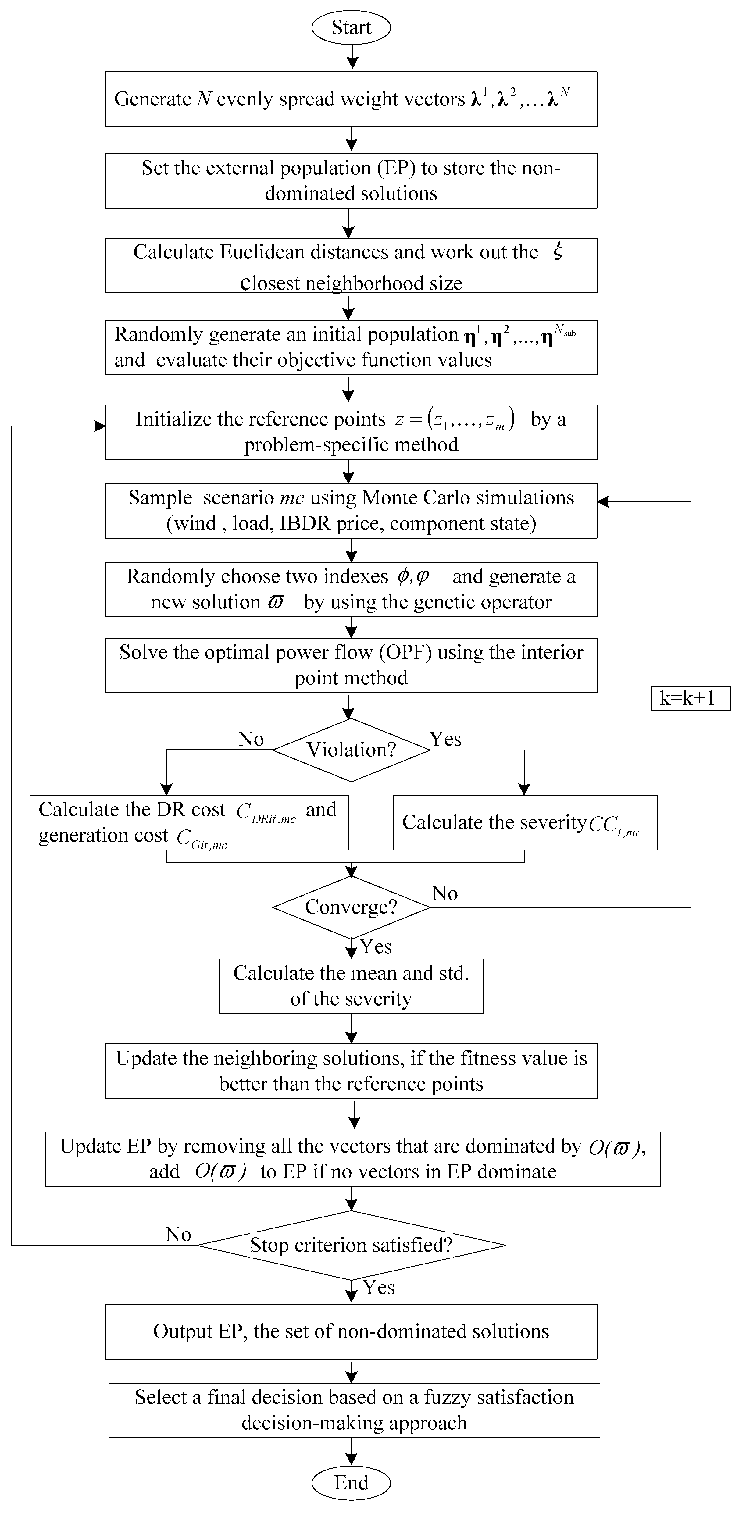
4.3. Solution Algorithm

Pareto optimality theory can define trade-off solutions. Given the feasible decision space η , a solution η * η , is called non-dominated or Pareto optimal if there does not exist another solution, η η , such that O ( η ) O ( η * ) , and O i ( η ) O i ( η * ) , for at least one function. None of the objective functions can be improved in value without impairment in some of the other objective values. The set of all the Pareto optimal solutions is called a Pareto set (PS), and the set of all the Pareto optimal objective vectors is the Pareto frontier (PF). A multi-objective evolutionary algorithm (MOEA) is widely used to approximate the PF [28].
For a multi-objective optimization problem (MOP) with m objectives, the Tchebycheff approach is adopted to decompose the MOP into N scalar optimization sub-problems by altering the weight vector λ = ( λ 1 , λ 2 , ... , λ m ) T , which is subject to λ i 0 , i [ 1 , m ] and i = 1 m λ i = 1 .
Minimize { ϑ t e ( η | λ j , z * ) = max 1 i m [ λ i j | O i ( η ) z i * | ] }
Subject   to   η Ω
where z * = ( z 1 * , z 2 * , ... , z m * ) T is the reference point vector. For a minimization problem, z i * = min { O i ( η ) | η Ω } , i [ 1 , m ] .
The key operations of MOEA/D are as follows, and the flow chart is shown in Figure 2. More information can be found in [29]. Note that this algorithm is open to parallel processing techniques, and hence computation time can be quasi-linearly reduced when necessary [30].
Step 1:
Initialization.
Step 1.1:
Generate N evenly spread weight vectors: λ 1 , λ 2 , λ N .
Step 1.2:
Set EP = Ø, where EP represents the external population, which is used to store non-dominated solutions found during each iteration.
Step 1.3:
Calculate Euclidean distances between any two weight vectors and then work out the ξ closest weight vectors of each weight vector. For the ith sub-problem, ∀i ∈ [1, Nsub], let set E ( i ) = { i 1 , i 2 , , i ξ } , where Nsub and λ i 1 , λ i 2 , ... , λ i ξ are number of sub-problems and the ξ closest weight vectors of λi, respectively.
Step 1.4:
Generate an initial population η 1 , η 2 , ... , η N sub randomly and then set O V i = O ( η i ) , where O V i represents the vector for objective function values of the ith sub-problem.
Step 1.5
Initialize z = ( z 1 , , z m ) by a problem-specific method.
Step 2:
Update solutions of sub-problems.
For i = 1 ,   2 , , N s u b , perform the following steps.
Step 2.1:
Reproduction. Randomly choose two indexes ϕ , φ from E(i) and then generate a new solution ϖ from η ϕ and η φ by using a specific operator (e.g., genetic operator).
Step 2.2:
Obtain the operation cost and calculate the risk value. Three tasks are completed in this step. (i) For each sampled scenario, solve the optimal power flow (OPF) by a state-of-the-art method (e.g., the interior point method). If no network constraint is violated, calculate the DR cost C D R i t , m c and generation cost C G i t , m c using (24) and (25). If there is any network violation, CC actions are used, and the severity C C t , m c is calculated by (29). (ii) When MC simulations converge, calculate the mean and Std. of the severity using (27) and (28). (iii) For a given k , calculate the risk value after risk aversion using (30)–(32).
Step 2.3:
Update of the neighboring solutions. For each index j E ( i ) , if ϑ t e ( ϖ | λ j , z * ) ϑ t e ( η j | λ j , z * ) , then set η j = ϖ and O V j = O ( ϖ ) .
Step 2.4:
Update of EP. Remove from EP all the vectors dominated by O ( ϖ ) . Add O ( ϖ ) to EP if no vectors in EP dominate.
Step 3:
Termination.
If convergence criterion is satisfied, stop the program and export the EP. Otherwise, go to Step 2. The termination criterion can be: the maximum iteration number is reached, or no changes are found in EP in a number of successive iterations.
Step 4:
Solution selection
With the obtained PF, a final solution can be selected according to practical needs, e.g., Nash equilibrium [31], minimizing the normalized Euclidian distance [21], individual risk preference or engineering judgments [3,32]. In this paper, a fuzzy satisfaction decision-making approach is adopted, and technical details regarding this approach can be found in [33].

5. Case Studies

5.1. Experimental Setting

The proposed approach is tested on the Garver’s six-bus, IEEE 24-bus RTS and 2383-bus Polish systems. Forced outage rates (FORs) of power-generating units and transmission lines and network data can be found in [34,35,36] respectively. We assume that the network needs to be expanded for the next five years, and the annual load growth rate is 5%. In other words, the load growth uncertainty in TEP is modeled as:
P D y e a r   5 = P D b a s e ( 1 + 5 % ) ^ 5 + Δ P D
where P D b a s e denotes the power load in the base year; P D y e a r   5 denotes the power load for the next five years while considering the load growth uncertainty; and Δ P D denotes the long-term load forecast uncertainty, which is assumed to follow a Gaussian distribution. In this paper, we only consider the long-term load growth uncertainty. The hourly load levels are proportionally allocated based on the forecasted peak load. The hourly load percentage to the peak load is calculated using the load profile of New South Wales, Australia, in the National Transmission Network Development Plan 2016 data, which can be found on [37].
The capacity of new power lines is 120 MW, and up to three lines are allowed on each corridor. The line investment cost is assumed to be 55 M$/100 km. DR resources are located at all load buses and the mean of IBDR cost can be found in [9]. The maximum ratio of IBDR is 10%. The cut-in, cut-out and rated speeds of wind turbines are 4.6 m/s, 25.8 m/s and 14.6 m/s. In the base case, is set to be 3. Value of customer reliability (VCR) is set to be $25,950/MWh [38].
The risks of incurring unreliability issues (e.g., involuntary load curtailments and generation corrective control actions) are considered as threat events to electricity network planners. The risk objective for the proposed approach is calculated using Equation (30), while the financial results are calculated using Equations (21)–(25). The simulations were completed by a PC with Intel Core i7-6600 CPU @ 2.80 GHZ with 8.00 GB RAM.

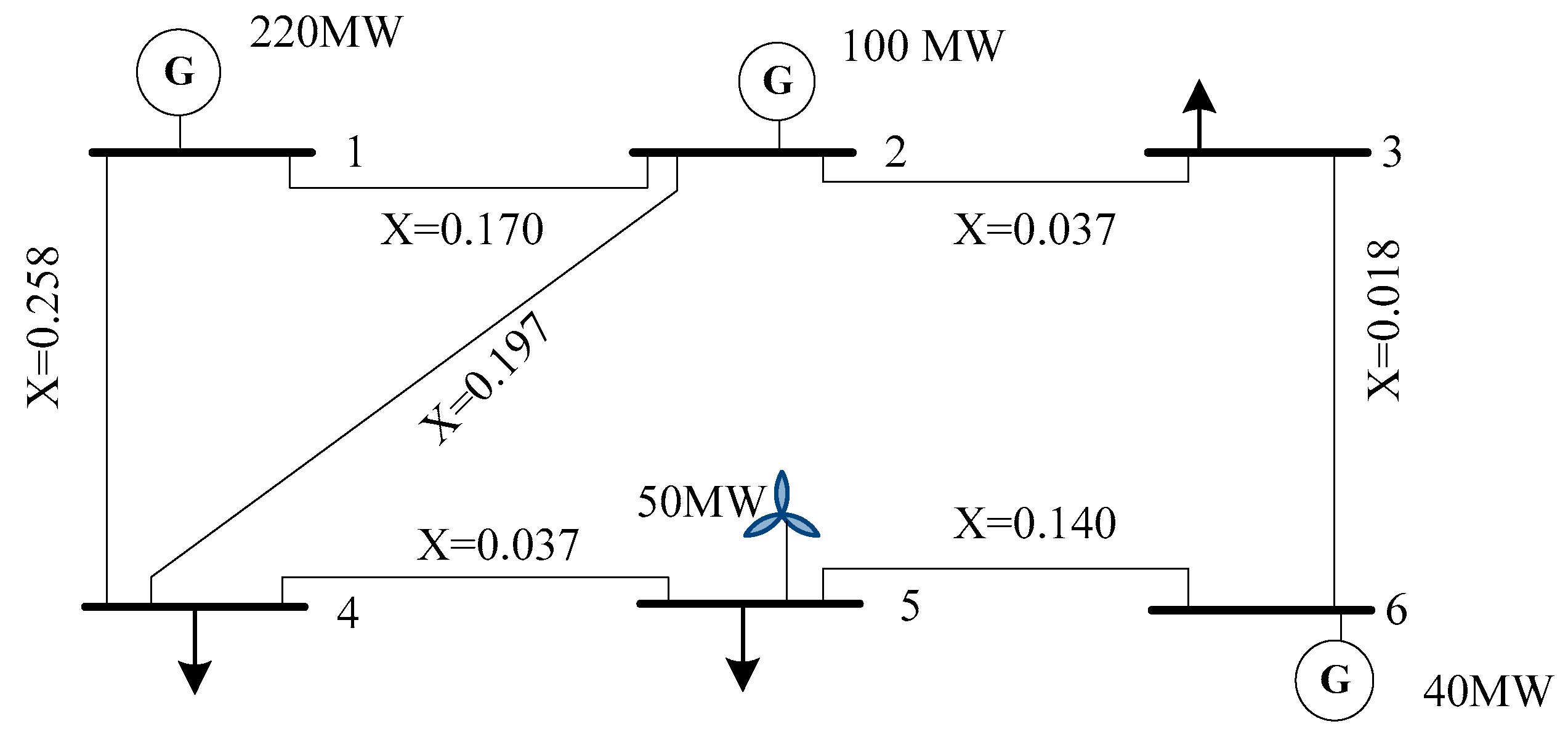
5.2. Garver’s 6-Bus System
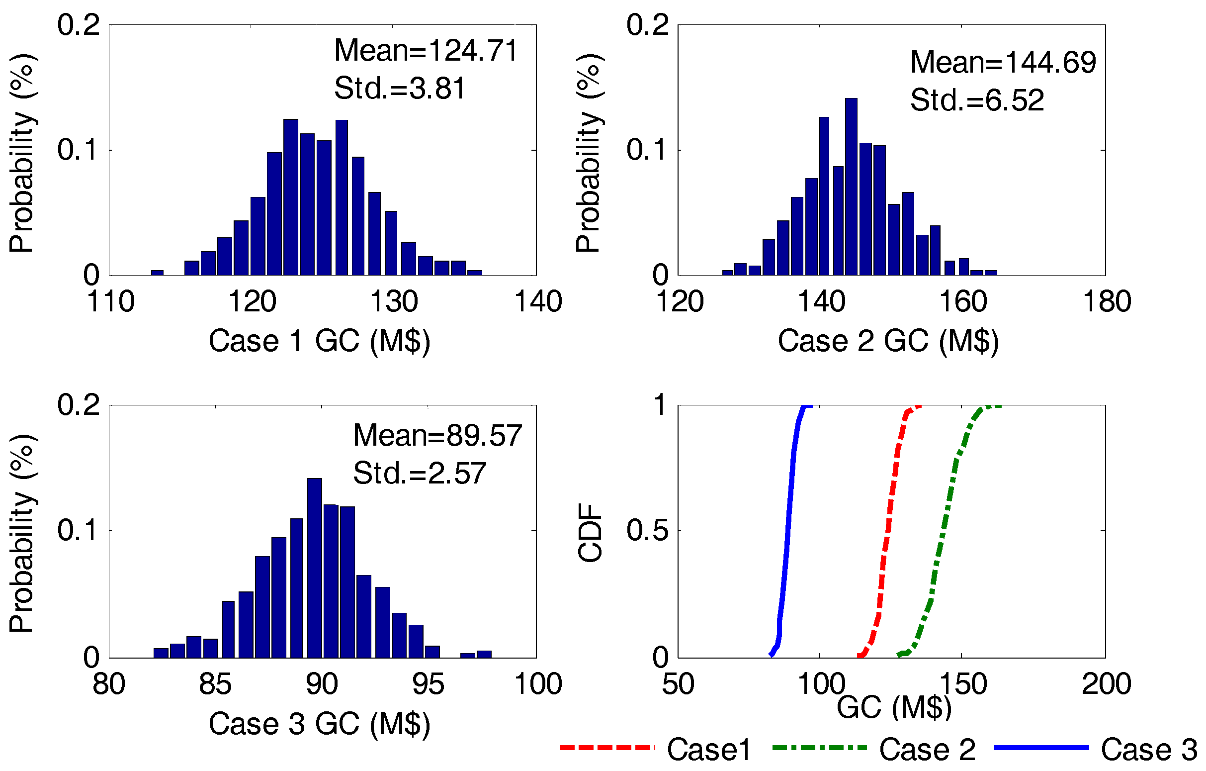
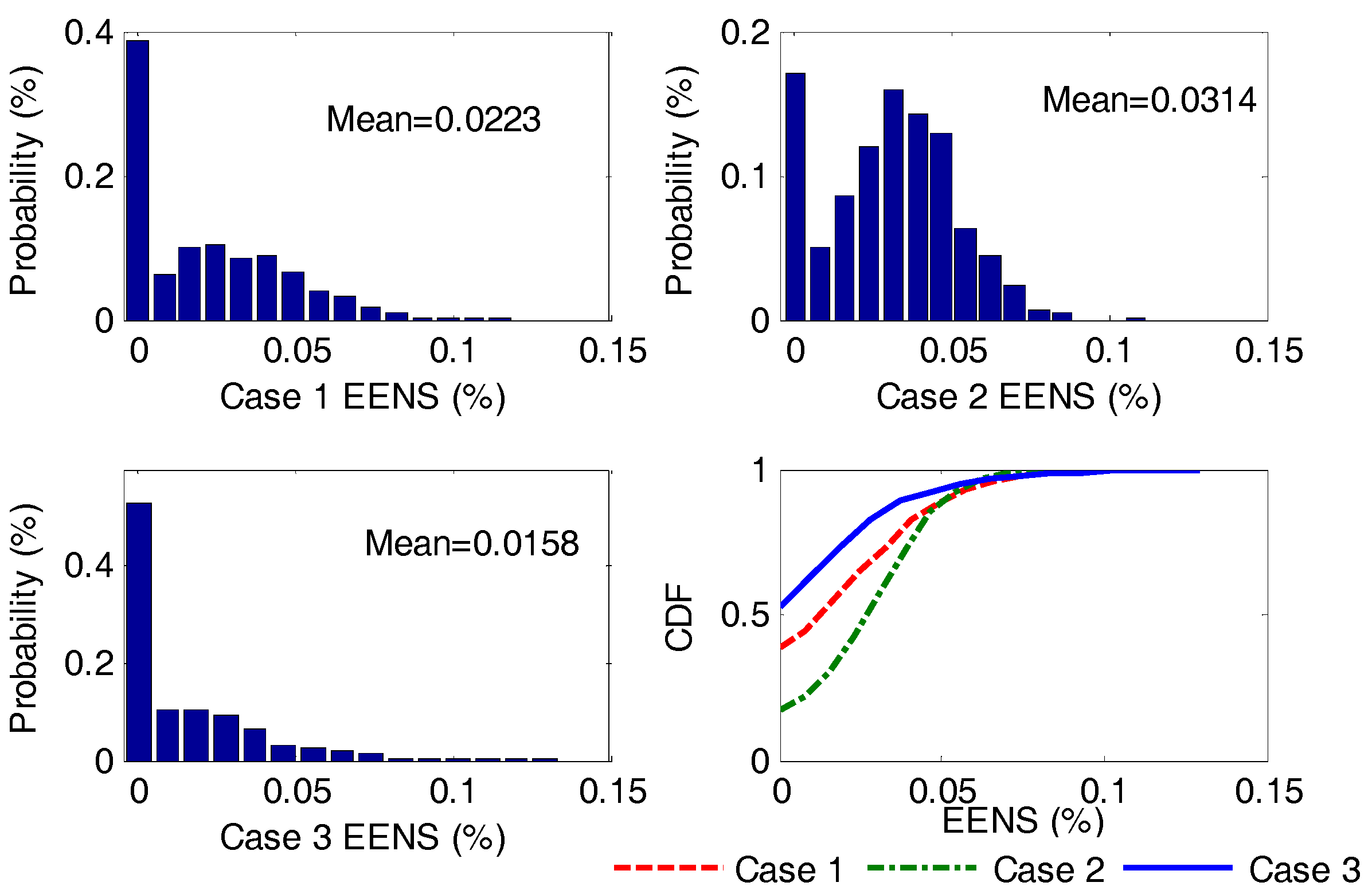
As seen in Figure 3, the six-bus system is composed of three thermal generators and one wind power unit, seven branches, and three loads. The peak load is 255 MW, and the total generation capacity is 410 MW. In the base case, wind power capacity is 50 MW. Wind power output, load, component availability and IBDR costs are considered as uncertainties.
Three cases are used to demonstrate the effectiveness of the proposed model.
Case 1:
The risk objective in (26) is not considered. A single objective TEP approach with a deterministic reliability constraint (i.e., E E N S E E N S max ) as reported in [39].
Case 2:
Similar to case 1, without the consideration of DR.
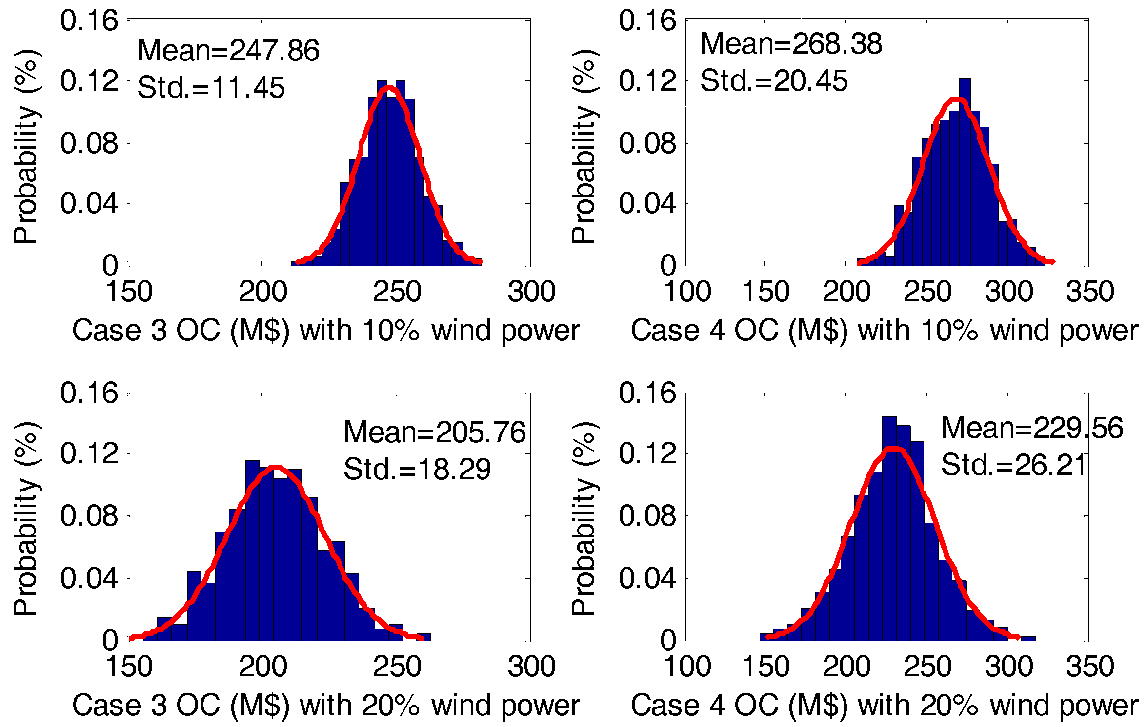
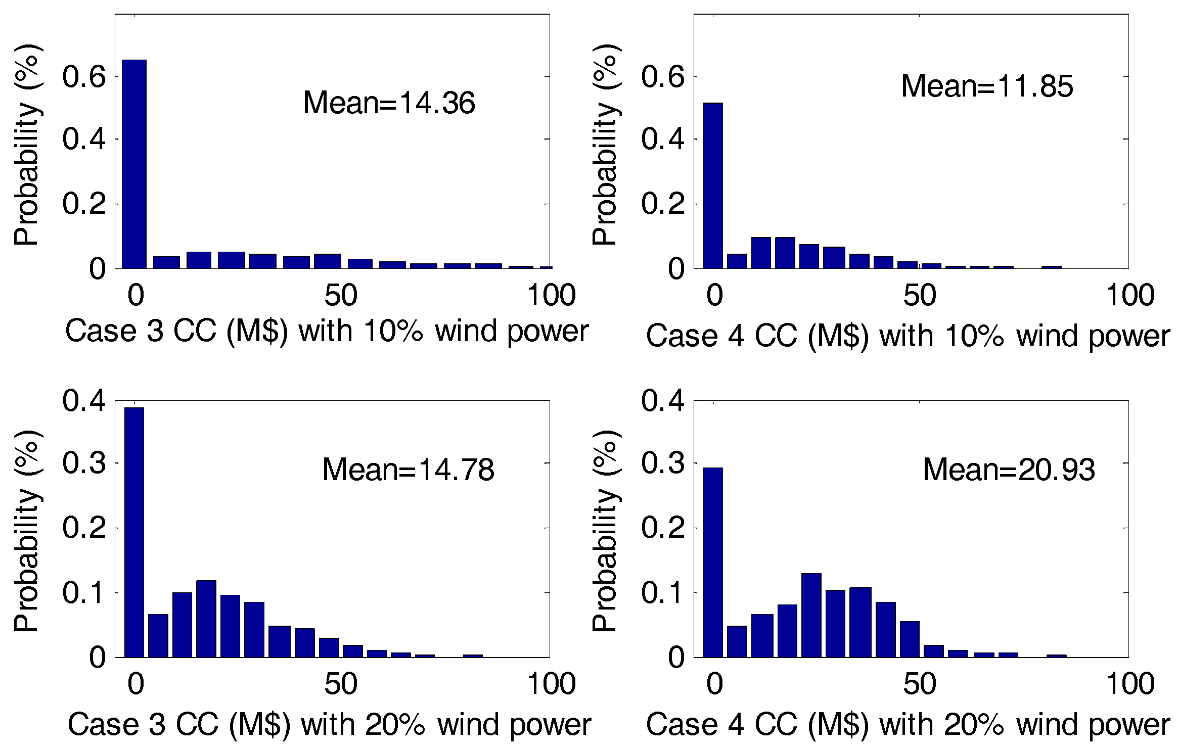
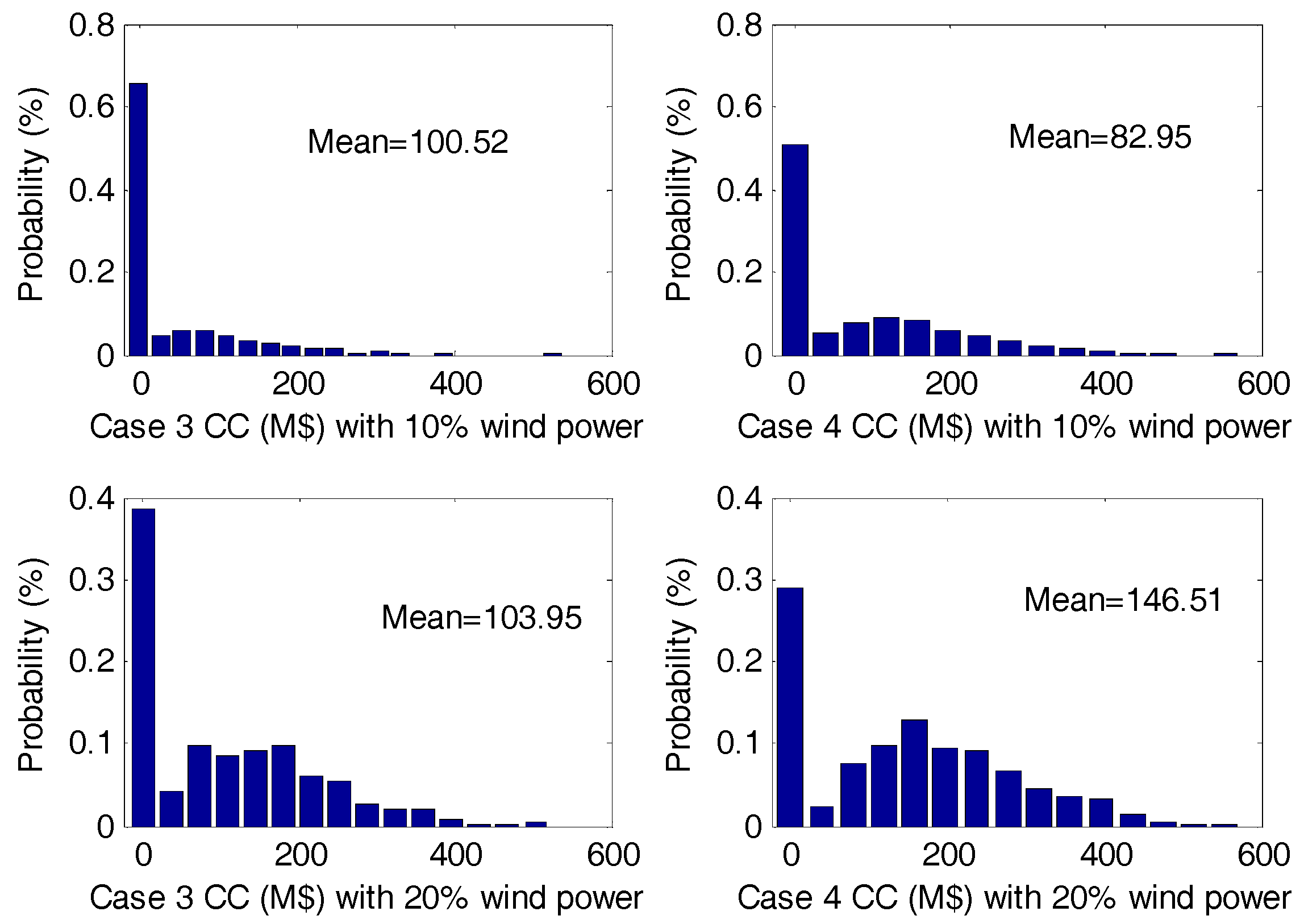
Case 3:
The proposed multi-objective TEP approach with DR and with the risk aversion strategy ( k is set to be 3).
The probability distributions of generation cost (GC) and the cumulative distribution function (CDF) for cases 1–3 are illustrated in Figure 4. Because the access to cheap generation resources can be guaranteed in case 3, the mean of GC is the lowest for case 3 (89.57 M$). Meanwhile, the lowest standard deviation (Std.) in case 3 (2.57 M$) implies that case 3 is less likely to be affected by the variations of uncertainties in our study. By contrast, the deterministic reliability constraint results in conservativeness, and more costly generating resources are used. Besides, DR plays an important role in enhancing the system economic efficiency, as the GC for case 1 is much lower compared with case 2 (124. 71 M$ vs. 144.69 M$). Moreover, we can see that case 3 is more useful in terms of hedging risks, since less extreme scenarios are observed (i.e., the tail distribution of CDF for case 3 is shorter). This means that the maximum financial loss due to load curtailments or CC actions in sampled scenarios is greatly reduced. The probability distribution of losses in Figure 1 is more concentrated near the mean, and the right tail is shortened. Therefore, the proposed method is superior to the previous work using the deterministic reliability constraint.
The detailed results including GC, DR cost (DRC), investment cost (IC), total cost and expected energy not supplied (EENS) for cases 1–3 are given in Table 1. Note that EENS is calculated by minimizing the total involuntary load curtailment under normal and contingency conditions ( E E N S = k = 0 K t = 1 8760 i Ω D P k i t C u r t ) [26]. For a deterministic approach, the planning criterion in this paper is defined as that EENS should be less than 0.02% of total annual energy consumption. As seen in Table 1, compared to case 1, although IC and DRC for case 3 are higher, the total cost and EENS are the lowest (256.44 M$ and 0.0156%). This is because low-cost DR and generation resources can be used more efficiently in case 3. Conversely, a deterministic TEP approach without DR leads to an inferior solution with high cost (310.16 M$), and low system reliability (EENS is 0.0196%). This means that DR can effectively reduce generation cost and improve system reliability, thus enhancing the network efficiency. To sum up, the adopted risk aversion strategy (when k = 3 ) has identified a planning solution that requires a higher investment, but the reinforced network is more reliable (lower EENS) and more cheap generation and DR resources can be used (lower GC and DRC). As a result, the total cost for case 3 is the lowest.
The wind power capacity at bus 5 is increased from 50 MW to 100 MW. Figure 5 illustrates the probability distributions of EENS and CDF with 100 MW wind power for cases 1–3. In general, more EENS is concentrated at 0 (see the CDF for distributions at 0). The distribution tail for case 2 is the biggest, followed by case 1, and then case 3. Meanwhile, the mean value also follows the same ranking. The results in Figure 5 indicate that in case 3, the low probability scenarios are less discounted, and the risk of unacceptable reliability is effectively hedged.
Furthermore, to investigate the influences of increasing wind power integration, results including total cost, total energy consumption, total wind power curtailment (WPC), peak load, and EENS under deterministic N-1 and N-2 contingencies are compared in Table 2 and Table 3. Table 2 presents more detailed information extended from Table 1 (wind power in base case is 50 MW), while Table 3 presents results with wind power of 100 MW. We can see that the growth in wind power penetration increases total cost, as the network needs to be reinforced and more DR is used to help absorb wind power. However, the increase in total cost can be effectively mitigated if the proposed TEP approach is used (for case 3, total cost is 256.44 M$ in Table 2, and 256.58 M$ in Table 3). Moreover, increasing wind power integration poses emerging security issues, as EENS sees rises for all cases. It is worth mentioning that only cases 3 can satisfy the 0.02% reliability criterion under N-1 and N-2 contingencies with higher wind power integration. Furthermore, higher WPC is observed in Table 3, but this rise is the slightest for case 3 (4.52 GWh in Table 2 and 4.56 GWh in Table 3). On the other hand, the increasing wind power has no impact on total energy consumption and peak load. From Table 2 and Table 3, we can see that the proposed risk aversion approach can effectively accommodate more wind power with the minimum impact on cost (total costs are 256.44 and 256.58 M$ for case 3 in Table 2 and Table 3 respectively) and system reliability (the N-2 EENS values are 0.0196% and 0.0199% for case 3 in Table 2 and Table 3 respectively).

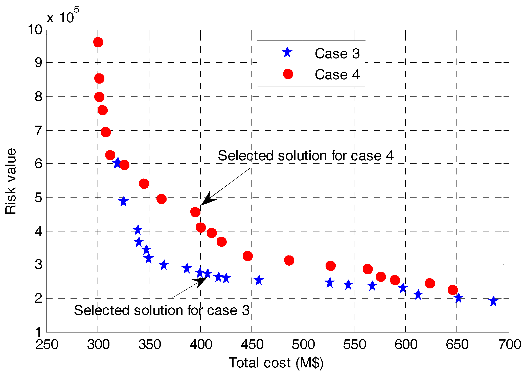
5.3. IEEE 24-Bus System

The IEEE 24-bus system is composed of 10 thermal stations, 38 branches and 20 loads. The peak load is 3650 MW, and the total generation capacity of thermal units is 6000 MW. We assume that three WP are located at buses 2, 4, and 20, and they have equal capacities at 200 MW (total WP at a 10% penetration level). One more case is added for comparison.
Case 4:
A multi-objective TEP approach without risk aversion. This means that in the optimization model, the second objective is (27), instead of (30).
The tradeoffs between risk value and cost for case 3 and 4 are shown in Figure 6. As seen, lower cost results in higher risk, and they are in conflict with each other. The multi-objective framework can provide network planners with a set of solutions (i.e., Pareto set). The selected solutions for cases 3 and 4 are marked in Figure 6. The identified planning schemes are given in Table 4. Generally, to attain a similar risk level, the total cost for case 4 is higher, compared with case 3.
In Table 5 and Table 6, results including total cost, risk value, WPC, peak load and EENS under deterministic N-1 and N-2 contingencies are compared between cases 3 and 4 for different wind power penetration. The total cost for case 3 is higher compared to case 4 in Table 5, but this is opposite when wind power penetration is increased to 20% in Table 6. Besides, risk value and EENS are always lower for case 3. This proves that the proposed approach is more cost-effective in terms of reducing risk and EENS. However, for WPC and peak load, the changes are not evident for both cases.
Figure 7 and Figure 8 illustrate probability distributions of operation cost (OC) and corrective control cost (CC) for different wind power penetration. As seen, increasing wind power reduces OC but increases Std. (from 11.45 to 18.29 for case 3 and from 20.45 to 26.21 for case 4). The increased Std. means increasing wind power introduces more uncertainty, thus, sophisticated system operation strategies are needed, such as more efficient use of DR, advanced wind forecast tools, risk management, etc. Moreover, the mean values of OC are lower for case 3, compared to case 4. With regard to CC, case 3 is higher with 10% wind, but becomes lower with 20% wind (14.78 M$ for case 3 and 20.93 M$ for case 4).
In addition, variations in total cost and CC corresponding to different risk preferences for case 3 are shown in Figure 9. A solution selected by a higher k is said to be risk averse; the opposite case is risk preferring. The higher value of k , the more concern about the higher CC with lower probabilities. In other words, higher k results in higher total cost, but lower CC. It is worth mentioning that lower CC implicitly means higher reliability, because CC actions refer to generation rescheduling and load curtailment under contingencies. The intersections of lines of different wind penetration levels in Figure 9 indicate that integrating more wind power does not always incur higher costs, on the condition that an appropriate k is selected. This means that a sophisticated risk-aversion strategy can effectively reduce the cost in relation to increasing wind power integration.

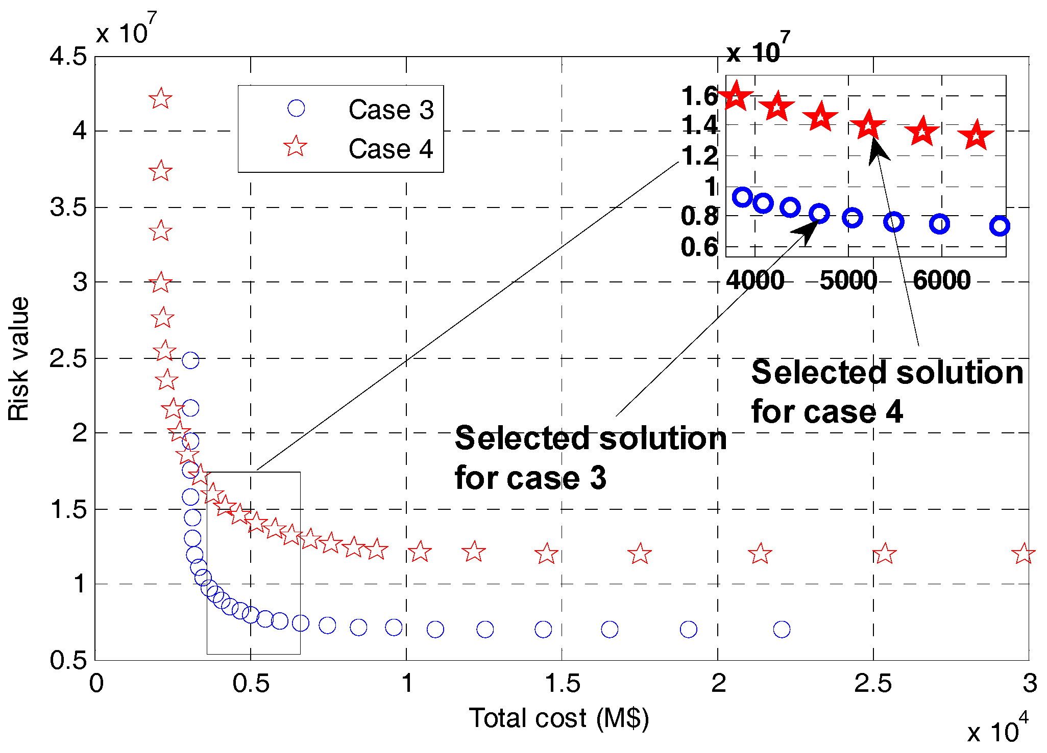
5.4. 2383-Bus Polish System

The peak load of the studied 2383-bus Polish system is 24,558 MW, and the total generation capacity is 38,179 MW. We assume that five WP farms are located at buses 64, 730, 1024, 1875 and 2204, with a total wind power penetration of about 10% (i.e., individual size is 760 MW, and a total of 3800 MW). To verify the effectiveness of the proposed risk aversion approach, cases 3 and 4 in Section 5.2 are compared.
Figure 10 illustrates the tradeoffs between total cost and risk value, and the selected solutions are marked. As seen in Figure 10, a lower total cost incurs a higher insecurity risk, meaning the two objectives conflict with each other. With a similar total cost, case 3 is more likely to incur lower risks, as the approximated Pareto frontier for case 3 is lower than that for case 4. For case 3, the range of total cost is between 3072 M$ and 22,076 M$, while the corresponding range of insecurity risk is between 6,922,194 and 24,733,345. For case 4, the range of total cost is between 2138 M$ and 29,922 M$, while the corresponding range of insecurity risk is between 11,919,876 and 42,075,351. We can see that if k is set at 3 in case 3, the maximum risk value is substantially reduced from 42,075,351 to 24,733,345, meaning about a 41% reduction. Usually, the maximum risk value means catastrophic threats. Therefore, we can conclude that the proposed risk aversion approach can identify planning solutions that are more resilient to extreme events, such as multiple line outages due to floods or ice storms in reality.
The distributions of CC costs for cases 3 and 4 with different wind power penetrations are shown in Figure 11. We can see that the increased wind power penetration has very little impact on the CC cost for case 3, while the mean of CC cost for case 4 substantially increases from 82.95 M$ to 146.51 M$, corresponding to about a 43% rise. This means that the proposed risk aversion approach can identify solutions that are more robust to wind uncertainty. Furthermore, the detailed results for cases 3 and 4 with 10% wind power for the Polish 2383-bus system are compared in Table 7. We can see that case 3 is superior in terms of economy and reliability. In addition, to show the scalability of the proposed approach, the computational performances on different sized power systems are compared in Table 8. The Polish 2383-bus system requires about 10 hours on a PC with Intel Core i7-6600 CPU @ 2.80 GHZ with 8.00 GB RAM. It should be noted that the contingency analysis based on Monte Carlo simulations accounts for almost half of the total time. This means that if parallel computing is used for contingency analysis, the solution algorithm can converge faster. Given that TEP problems aim to identify network expansion solutions for a future scenario (e.g., 5 or 10 years ahead), the solution time required in this paper is reasonable.
More importantly, this paper has proposed a risk index that can quantitatively measure the system reliability under extreme scenarios. The identified solutions can effectively reflect how much a decision-maker is concerned about the low-probability but high-loss threats in planning practices. The formulated multi-objective risk aversion planning model can help network planners better comprehend the options they have, and the risk that each option entails. To sum up, the proposed model is a flexible decision-making tool, which can help decision-makers make tradeoffs between economy and reliability.

6. Conclusions

This paper presents a probabilistic multi-objective TEP model for power systems with increasing wind power integration. The unacceptable reliability risk is proposed based on the probability of contingencies and the corresponding cost of corrective control actions. The proposed risk value formulation can be easily adjusted according to the individual risk preferences of decision-makers. Thus, the formulated objective function includes costs of investment, power generation, DR and the unacceptable reliability risk. In addition, the MOEA/D is introduced and employed to find Pareto optimal solutions of the proposed TEP model. According to case studies, the deterministic TEP approach results in inferior solutions with high cost and low system reliability. Also, increasing wind power integration will increase the overall system cost and the risk of reliability issues, but this effect can be mitigated if a risk-aversion strategy is adopted. Therefore, the proposed method in this paper still enforces the reliability criterion, and is superior to the deterministic version and the version without DR. In conclusion, the proposed approach is a useful decision-making tool, which allows flexible risk analysis.

Acknowledgment

The work in this paper is supported by a China Southern Power Grid Research Grant WYKJ00000027, the National Natural Science Foundation of China (Key Program 71331001, 71420107027 and General Program 71071025, 71271033) and the Shenzhen Municipal Science and Technology Innovation Committee International R&D project (GJHZ20160301165723718).

Author Contributions

Jing Qiu did the simulation work and wrote the manuscript. Junhua Zhao and Dongxiao Wang checked the model and proofread the manuscript.

Conflicts of Interest

The authors declare no conflict of interest.

Nomenclature

DefinitionsSymbolsDescriptions
Risk attitude factor k An index that measures to what extent a decision-maker cares about the risk below (when k < 0 ) or above the expected risk value (when k > 0 ).
Probability of risk aversion α A probability that measures the occurrence frequency of threats due to a risk-aversion strategy. Theoretically, when α 1 , a decision-maker incurs no risk; when α 0 , a decision-maker adopts no risk aversion strategies, thus incurring business-as-usual risks.
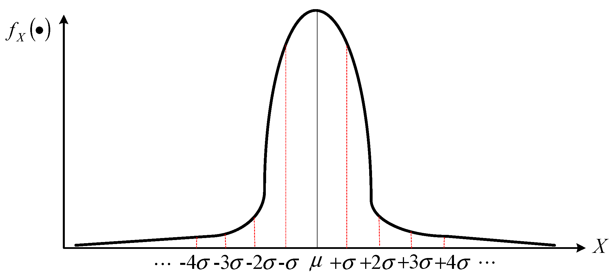
Probability density function of the risk attitude factor f K ( ) A function used to specify the probability of the risk attitude factor falling within a particular range of values. This probability density function (PDF) is defined to represent the catastrophic consequences of a low-probability threat event to power networks.
Risk value after risk aversion R K A defined risk value that has taken into account the risk attitude factor and the probability of risk aversion, as well as the probability and the severity of threat events.

References

  1. Munoz, C.; Sauma, E.; Contreras, J.; Aguado, J.; de la Torre, S. Impact of high wind power penetration on transmission network expansion planning. IET Gener. Trans. Distrib. 2012, 6, 1281–1291. [Google Scholar] [CrossRef]
  2. Ugranli, F.; Karatepe, E. Multi-objective transmission expansion planning considering minimization of curtailed wind energy. Int. Electr. Power Energy Syst. 2015, 65, 348–356. [Google Scholar] [CrossRef]
  3. Javadi, M.S.; Saniei, M.; Mashhadi, H.R.; Gutierrez-Alcaraz, G. Multi-objective expansion planning approach: Distant wind farms and limited energy resources integration. IET Renew. Power Gener. 2013, 7, 652–668. [Google Scholar] [CrossRef]
  4. Hamon, C.; Perninge, M.; Soder, L. An importance sampling technique for probabilistic security assessment in power systems with large amounts of wind power. Electr. Power Syst. Res. 2016, 131, 11–18. [Google Scholar] [CrossRef]
  5. Park, H.; Baldick, R. Transmission planning under uncertainties of wind and load: Sequential approximation approach. IEEE Trans. Power Syst. 2013, 28, 2395–2402. [Google Scholar] [CrossRef]
  6. Billinton, R.; Wangdee, W. Reliability-based transmission reinforcement planning associated with large-scale wind farms. IEEE Trans. Power Syst. 2007, 22, 34–41. [Google Scholar] [CrossRef]
  7. Orfanos, G.A.; Georgilakis, P.; Hatziargyriou, N.D. Transmission expansion planning of systems with increasing wind power integration. IEEE Trans. Power Syst. 2013, 28, 1355–1362. [Google Scholar] [CrossRef]
  8. Kamalinia, S.; Shahidehpour, M.; Khairuddin, A. Security-constrained expansion planning of fast-response units for wind integration. Electr. Power Syst. Res. 2011, 81, 107–116. [Google Scholar] [CrossRef]
  9. Li, C.X.; Dong, Z.Y.; Chen, G.; Luo, F.J.; Liu, J. Flexible transmission expansion planning associated with large-scale wind farms integration considering demand response. IET Gener. Trans. Distrib. 2015, 9, 2276–2283. [Google Scholar] [CrossRef]
  10. Gan, L.; Li, G.; Zhou, M. Coordinated planning of large-scale wind farm integration system and regional transmission network considering static voltage stability constraints. Electr. Power Syst. Res. 2016, 136, 298–308. [Google Scholar] [CrossRef]
  11. Rahimi, F.; Ipakchi, A. Demand response as a market resource under the smart grid paradigm. IEEE Trans. Smart Grid 2010, 1, 82–88. [Google Scholar] [CrossRef]
  12. Nguyen, D.T.; Negnevitsky, M.; Groot, M.d. Market-based demand response scheduling in a degregulated environment. IEEE Trans. Smart Grid 2013, 4, 1948–1956. [Google Scholar] [CrossRef]
  13. Hinojosa, V.H.; Nuques, G.B. A simulated rebounding algorithm applied to the multi-stage security-constrained transmission expansion planning in power systems. Int. J. Electr. Power Energy Syst. 2013, 47, 168–180. [Google Scholar] [CrossRef]
  14. Foroud, A.A.; Abdoos, A.A.; Keypour, R.; Amirahmadi, M. A multi-objective framework for dynamic transmission expansion planning in competitive electricity market. Int. J. Electr. Power Energy Syst. 2010, 32, 861–872. [Google Scholar] [CrossRef]
  15. Akbari, T.; Rahimi-Kian, A.; Bina, M.T. Security-constrained transmission expansion planning: A stochastic multi-objective approach. Int. J. Electr. Power Energy Syst. 2012, 43, 444–453. [Google Scholar] [CrossRef]
  16. Florez, C.A.C.; Ocampo, R.A.B.; Zuluaga, A.H.E. Multi-objective transmission expansion planning considering multiple generation scenarios. Int. J. Electr. Power Energy Syst. 2014, 62, 398–409. [Google Scholar] [CrossRef]
  17. Yu, H.; Chung, C.Y.; Wong, K.P.; Zhang, J.H. A chance constrained transmission network expansion planning method with consideration of load and wind farm uncertainties. IEEE Trans. Power Syst. 2009, 24, 1568–1576. [Google Scholar] [CrossRef]
  18. Villumsen, J.C.; Bronmo, G.; Philpott, A.B. Line capacity expansion and transmission switching in power systems with large-scale wind power. IEEE Trans. Power Syst. 2013, 28, 731–739. [Google Scholar] [CrossRef]
  19. Taherkhani, M.; Hosseini, S.H. Wind farm optimal connection to transmission systems considering network reinforcement using cost-reliability analysis. IET Renew. Power Gener. 2013, 7, 603–613. [Google Scholar] [CrossRef]
  20. Moeini-Aghtaie, M.; Abbaspour, A.; Fotuhi-Firuzabad, M. Incorporating large-scale distant wind farms in probabilistic transmission expansion planning-part i: Theory and algorithm. IEEE Trans. Power Syst. 2012, 27, 1585–1593. [Google Scholar] [CrossRef]
  21. Arabali, A.; Ghofrani, M.; Etezadi-Amoli, M.; Fadali, M.S.; Moeini-Aghtaie, M. A multi-objective transmission expansion planning framework in deregulated power systems with wind generation. IEEE Trans. Power Syst. 2014, 29, 3003–3011. [Google Scholar] [CrossRef]
  22. Ozdemir, O.; Munoz, F.D.; Ho, J.L.; Hobbs, B.F. Economic analysis of transmission expansion planning with price-responsive demand and quadratic losses by successive lp. IEEE Trans. Power Syst. 2016, 31, 1096–1107. [Google Scholar] [CrossRef]
  23. Rockafellar, R.T.; Uryasev, S. Optimization of conditional value-at-risk. J. Risk 2000, 2, 21–41. [Google Scholar] [CrossRef]
  24. Eydeland, A.; Wolyniec, K. Energy and Power Risk Management; Wiley: Chichester, UK, 2003. [Google Scholar]
  25. Zhao, J.H.; Wen, F.S.; Dong, Z.Y.; Yue, Y.S.; Wong, K.P. Optimal dispatch of electric vehicles and wind power using enhanced particle swarm optimization. IEEE Trans. Ind. Inform. 2012, 8, 889–899. [Google Scholar] [CrossRef]
  26. Billinton, R.; Allan, R. Reliability Evaluation of Power Systems, 2nd ed.; Plenum Press: New York, NY, USA, 1996. [Google Scholar]
  27. Abdi, H.; Dehnavi, E.; Mohammadi, F. Dynamic economic dispatch problem integrated with demand response (DEDDR) considering non-linear responsive load models. IEEE Trans. Smart Grid 2016, 7, 2586–2595. [Google Scholar] [CrossRef]
  28. Ganguly, S.; Sahoo, N.C.; Das, D. Multi-objective planning of electrical distribution systems using dynamic programming. Int. J. Electr. Power Energy Syst. 2013, 46, 65–78. [Google Scholar] [CrossRef]
  29. Zhang, Q.; Li, H. A multiobjective evolutionary algorithm based on decomposition. IEEE Trans. Evol. Comput. 2007, 11, 712–731. [Google Scholar] [CrossRef]
  30. Xu, Y.; Dong, Z.Y.; Luo, F.; Zhang, R.; Wong, K.P. Parallel-differential evolution approach for optimal event-driven load shedding against voltage collapse in power systems. IET Gener. Trans. Distrib. 2014, 8, 651–660. [Google Scholar] [CrossRef]
  31. Xu, Y.; Dong, Z.Y.; Meng, K.; Yao, W.F.; Zhang, R.; Wong, K.P. Multi-objective dynamic var planning against short-term voltage instability using a decomposition-based evolutionary algorithm. IEEE Trans. Power Syst. 2014, 29, 2813–2822. [Google Scholar] [CrossRef]
  32. Maghouli, P.; Hosseini, S.H.; Buygi, M.O.; Shahidehpour, M. A scenario-based multi-objective model for multi-stage transmission expansion planning. IEEE Trans. Power Syst. 2011, 26, 470–478. [Google Scholar] [CrossRef]
  33. Maghouli, P.; Hosseini, S.H.; Buygi, M.O.; Shahidehpour, M. A multi-objective framework for transmission expansion planning in deregulated environments. IEEE Trans. Power Syst. 2009, 24, 1051–1061. [Google Scholar] [CrossRef]
  34. Wu, H.; Shahidehpour, M.; Al-Abdulwahab, A. Hourly demand response in day-ahead scheduling for managing the variability of renewable energy. IET Gener. Trans. Distrib. 2013, 7, 226–234. [Google Scholar] [CrossRef]
  35. IEEE Reliability Test System. Reliability test system task force of probability methods sub-committee. IEEE Trans. Power Appar. Syst. 1979, 98, 2047–2054. [Google Scholar]
  36. Matpower 5.0-Description of Case 2383wp. Available online: http://www.pserc.cornell.edu/matpower/docs/ref/matpower5.0/case2383wp.html (accessed on 14 July 2017).
  37. National Transmission Network Development Plan (NTNDP) Database, Aemo. Available online: https://www.aemo.com.au/Electricity/National-Electricity-Market-NEM/Planning-and-forecasting/National-Transmission-Network-Development-Plan/NTNDP-database (accessed on 14 July 2017).
  38. Australian Energy Market Operator (AEMO)-Value of Customer Reliability (VCR) Review. Available online: http://www.aemo.com.au/Electricity/National-Electricity-Market-NEM/Planning-and-forecasting/Value-of-Customer-Reliability-review (accessed on 17 July 2017).
  39. Zhao, J.H.; Dong, Z.Y.; Lindsay, P.; Wong, K.P. Flexible transmission expansion planning with uncertainties in an electricity market. IEEE Trans. Power Syst. 2009, 24, 479–488. [Google Scholar] [CrossRef]
Figure 1. Concept of the defined risk attitude factor (RAF).
Energies 10 01036 g001
Figure 2. Flow chart of the applied solution algorithm.
Energies 10 01036 g002
Figure 3. One-line diagram of six-bus system.
Energies 10 01036 g003
Figure 4. Probability distributions of generation cost (GC) and cumulative distribution function (CDF) for cases 1–3.
Energies 10 01036 g004
Figure 5. Probability distributions of expected energy not supplied (EENS) and CDF for cases 1–3 with 100 MW wind power penetration.
Energies 10 01036 g005
Figure 6. Tradeoffs between cost and risk for cases 3 and 4 for IEEE 24-bus system.
Energies 10 01036 g006
Figure 7. Operation cost (OC) distributions for cases 3 and 4 with increasing wind power.
Energies 10 01036 g007
Figure 8. Corrective control cost (CC) distributions for cases 3 and 4 with increasing wind power.
Energies 10 01036 g008
Figure 9. Variations in total cost and corrective control cost (CC) corresponding to different k for case 3.
Energies 10 01036 g009
Figure 10. Tradeoffs between cost and risk for cases 3 and 4 for the Polish 2383-bus system.
Energies 10 01036 g010
Figure 11. CC distributions for cases 3 and 4 with increasing wind power for the Polish 2383-bus system.
Energies 10 01036 g011
Table 1. Detailed results for cases 1–3.
Case #GC
(M$)
DRC
(M$)
IC
(M$)
Total Cost
(M$)
EENS
(%)
1124.716.59136.22267.520.0194
2144.69-165.47310.160.0196
389.5710.26156.61256.440.0156
Table 2. Result comparison for cases 1–3 with 50 MW wind power.
Case #Total Cost
(M$)
Energy
(GWh)
WPC
(GWh)
Peak Load
(MW)
EENS (%)
N-1N-2
1267.52105.686.82299.410.01970.0234
2310.16103.4513.65325.450.01990.0365
3256.44106.364.52292.910.01620.0196
Table 3. Result comparison for cases 1–3 with 100 MW wind power.
Case #Total Cost
(M$)
Energy
(GWh)
WPC
(GWh)
Peak Load
(MW)
EENS (%)
N-1N-2
1275.21105.688.93299.410.01990.0264
2336.36103.4515.65325.450.02610.0398
3256.58106.364.56292.910.01970.0199
Table 4. Planning results for cases 3 and 4.
Case #Identified Planning Schemes
3 η 1 2 = 2 , η 1 5 = 1 , η 3 24 = 2 , η 5 10 = 1 , η 9 11 = 2 , η 11 14 = 1 , η 15 16 = 2 , η 17 22 = 2 , η 19 20 = 1 , η 20 23 = 1
4 η 1 3 = 1 , η 2 4 = 3 , η 4 9 = 2 , η 8 9 = 1 , η 13 23 = 1 , η 14 16 = 3 , η 15 21 = 1 , η 17 18 = 2 , η 18 21 = 2 , η 19 20 = 1 , η 21 22 = 2
Table 5. Results comparison for cases 3 and 4 with 10% wind power.
Case #Total Cost
(M$)
Risk
Value
WPC
(GWh)
Peak Load
(MW)
EENS (%)
N-1N-2
3418.26260,99530.544192.650.01690.0185
4395.18456,23642.364192.650.01720.0189
Table 6. Results comparison for cases 3 and 4 with 20% wind power.
Case #Total Cost
(M$)
Risk
Value
WPC
(GWh)
Peak Load
(MW)
EENS (%)
N-1N-2
3419.86303,38530.634192.650.01880.0194
4420.34652,36544.894192.650.01960.0215
Table 7. Results comparison for cases 3 and 4 with 10% wind power for the Polish 2383-bus system.
Case #Total Cost
(M$)
Risk
Value
WPC
(GWh)
EENS (%)
N-1N-2
35049.157,898,3211098.430.01760.0184
45223.4213,975,8762009.480.01880.0199
Table 8. Computational performances on different tested systems.
Tested SystemsTotal Elapsed (s)Contingency Analysis Elapsed (s)Iteration Number
6-bus6092452345
IEEE 24-bus14,65476434567
Polish 2383-bus37,87418,9847654

