Health Parameter Estimation with Second-Order Sliding Mode Observer for a Turbofan Engine

Abstract

In this paper the problem of health parameter estimation in an aero-engine is investigated by using an unknown input observer-based methodology, implemented by a second-order sliding mode observer (SOSMO). Unlike the conventional state estimator-based schemes, such as Kalman filters (KF) and sliding mode observers (SMO), the proposed scheme uses a “reconstruction signal” to estimate health parameters modeled as artificial inputs, and is not only applicable to long-time health degradation, but reacts much quicker in handling abrupt fault cases. In view of the inevitable uncertainties in engine dynamics and modeling, a weighting matrix is created to minimize such effect on estimation by using the linear matrix inequalities (LMI). A big step toward uncertainty modeling is taken compared with our previous SMO-based work, in that uncertainties are considered in a more practical form. Moreover, to avoid chattering in sliding modes, the super-twisting algorithm (STA) is employed in observer design. Various simulations are carried out, based on the comparisons between the KF-based scheme, the SMO-based scheme in our earlier research, and the proposed method. The results consistently demonstrate the capabilities and advantages of the proposed approach in health parameter estimation.

1. Introduction

In aircraft turbofan engine operations, reliability and efficiency are of utmost importance. Subjected to harsh environments, the gas-path performance of aero-engines gradually deteriorates over flights. Common causes of gradual degradation include the increase of the blade-tip clearance in the turbine, wear and erosion, the compressor fouling, and corrosion in hot sections. Besides, abrupt performance degeneration may happen due to foreign-object damage, such as birds, pieces of ice, and runaway debris. To manage a collection of such assets, the accurate estimation of current engine performance and fast diagnosis of machinery faults are necessary to maintain flight safety and reduce operating costs [1].

Gas-path related analyses have been effective in detecting faults in turbo machinery [2]. The variations of efficiency and flow capacity of rotary components, called “health parameters”, capture the nature of engine performance. They deviate from the nominal baseline gradually with time as engine parts wear from regular usage, and also abruptly due to component fault events. The health parameters provide crucial information for operating an aero-engine in a safe and efficient manner, but they cannot be directly measured during the flight [3]. Fortunately, the deterioration causes changes in sensed measurements. The goal of gas path health monitoring (GPHM) is to relate observed changes in measurements to internal changes in health parameters, to provide performance trend monitoring, which will be further used in engine fault diagnostics.

Various algorithms have been proposed to the GPHM, which can be classified as model-based algorithms (such as observers and filters) and data-driven algorithms (such as fuzzy logic [4], neural networks [5] and genetic algorithms [6]). Common model-based approaches to estimate health parameters are Weighted Least Squares [7], Generalized Observer [8] and Kalman filter [9,10]. Kalman filter approaches seem to be the most well-known methods for GPHM design. With health parameters treated as state variables, the linear Kalman filter is employed to optimally estimate state variations for on-board in-flight applications. Litt proposed a real-time Kalman filter approach for estimating helicopter engine degradation due to compressor erosion [11]. Simon D.L. developed a systematic sensor selection approach for on-board engine models for health monitoring use [12]. Lu reported an improved extended Kalman filter with inequality constraints for gas turbine engine health monitoring [13]. In general, the use of model-based approaches will inevitably lead to challenges due to model mismatches, which are not considered in the researches mentioned above. In view of this, some researchers proposed a unique hybrid model (eSTORM) that fused the self-tuning on-board real-time model (STORM) with an empirical neural net model [14,15], to provide modeling error compensation. However, the neural net is built based on off-line calculation and large amounts of flight data, which is laborious and time-consuming. Among the KF-based methods, it worth noting that they are under the assumption that performance deterioration is slowly evolving, and health parameters are modeled without dynamics. As a result, the Kalman filter responds in a sluggish manner in rapid or abrupt performance changes [16].

Recently there has been a wide interest in exploiting sliding mode observer techniques in the field of fault diagnosis. Due to the property of the discontinuous switched term, when a sliding motion is induced the observer is able to robustly estimate states/faults considering uncertainties. Thus sliding mode observer has been widely used in robust state estimation [17,18,19], constructing fault detection and isolation (FDI) scheme [20], detecting actuator faults [21] and handling sensor faults [22,23,24]. One problem of using sliding modes is the system chattering, however, since there is no output execution, the chattering is acceptable so long as it does not blur the observation results. Another problem is that the considered uncertainties in traditional sliding modes are restricted to be in a certain form, which is not realistic. Besides, in most of related work, robust fault diagnosis can be achieved only when the available measurements outnumber the faults, but in some applications this assumption is hard to meet and assuming “non-faulty sensors” inevitably reduce the system reliability. So far uses of SMO in fault detection have mainly been in handling actuator/sensor fault cases, but in our previous research, an aircraft engine health estimation system based on SMO was investigated [25]. The proposed scheme in [25] performs superior over the KF-based scheme with model mismatches considered, but some problems remain unsettled: one is the health parameters are still modeled without dynamics, like that in KF-based scheme; and another is the harsh restriction on allowed uncertainties, i.e., the uncertainty distribution matrix is forced to be in a certain form, which is hard to meet practically.

In this paper, an approach based on a second-order sliding mode observer is investigated for the estimation of health parameters in a civil aero-engine. Other than being as state variables like those in KF-based scheme, health parameters are modeled as unknown inputs, thus the assumption that health parameters are without dynamics is no more required, which results in a much quicker diagnosis speed. To solve the problem that the involved engine contains equal number of available sensors and health parameters, a transformation is introduced to create a fictitious output that dimensionally exceeds the health parameter vector, which make it possible for the robust observer design. Then the super-twisting algorithm is utilized to construct a second-order sliding mode observer, to ensure the sliding surface can be reached regardless of uncertainties. Also the high switching chattering is attenuated via the 2-order sliding mode methodology. Once sliding motion is achieved, a weighting matrix is designed to minimize the disturbance effect on the health estimation via linear matrix inequalities (LMI). Since robustly reaching the sliding surface is ensured by super-twisting algorithm and robustly estimation after sliding reaching is enabled by the weighting matrix, there is no any restrictions on uncertainty formulation.

This paper is organized as follows: First, the system description and transformation of the linear engine model are described, to make preparation for the observer design. Next, the SOSMO approach is introduced and the overall GPHM architecture is depicted. Then, the proposed method is verified in a nonlinear engine model with different deterioration scenarios. Finally, conclusions are presented.

2. System Description and Transformation

This paper is concerned with the design of a sliding mode observer for an uncertain state variable model (SVM) of an aero-engine subject to health degradation. A SVM of a steady-state operating point that subjected to health degradation and uncertainties is represented by

$$\begin{gathered} \dot{\mathit{x}}\left(t\right)=\mathit{A}\mathit{x}\left(t\right)+\mathit{B}\mathit{u}\left(t\right)+\mathit{L}\mathit{h}\left(t\right)+{\mathit{Q}}_1\mathit{\xi }\left(t\right) \\ \mathit{y}\left(t\right)=\mathit{C}\mathit{x}\left(t\right)+\mathit{D}\mathit{u}\left(t\right)+\mathit{M}\mathit{h}\left(t\right)+{\mathit{Q}}_2\mathit{\xi }\left(t\right), \end{gathered}$$

(1)

where $\mathit{x}={\left[N_{\mathrm{L}},N_{\mathrm{H}}\right]}^{\mathrm{T}}$, $\mathit{u}={\left[W_{\mathrm{f}},{\theta }_{\mathrm{VSV}},{\mathsf{\theta }}_{\mathrm{VBV}}\right]}^{\mathrm{T}}$, and $\mathit{y}={\left[N_{\mathrm{L}},N_{\mathrm{H}},P_{25},T_{25},P_3,T_3,T_{495}\right]}^{\mathrm{T}}$ are the state variables, the known inputs and the outputs, respectively. $\mathit{h}={\left[h_1,h_2,..,h_7\right]}^{\mathrm{T}}$ stands for the health parameters, which can be regarded as unknown inputs. $\mathit{A}\in {ℝ}^{n\times n}$, $\mathit{B}\in {ℝ}^{n\times m}$, $\mathit{C}\in {ℝ}^{p\times n}$, $\mathit{D}\in {ℝ}^{p\times m}$, $\mathit{L}\in {ℝ}^{n\times q}$, and $\mathit{M}\in {ℝ}^{p\times q}$ are constant coefficient matrices. Here, $n=2$, $m=3$, $p=7$, $q=7$. ${\mathit{Q}}_{\mathbf{1}}\in {ℝ}^{n\times r}$ and ${\mathit{Q}}_{\mathbf{2}}\in {ℝ}^{p\times r}$ represent the uncertainty distribution matrix, while $\mathit{\xi }\left(\mathit{t}\right)\in {ℝ}^{r\times 1}$ denotes uncertainties. Assume $\mathit{h}\left(t\right)$, $\mathit{\xi }\left(t\right)$ and their first time derivatives are unknown but bounded

$$\Vert \mathit{\xi }\left(t\right)\Vert <{\alpha }_1,\Vert \dot{\mathit{\xi }}\left(t\right)\Vert <{\alpha }_2,\Vert \mathit{h}\left(t\right)\Vert <{\beta }_1,\Vert \dot{\mathit{h}}\left(t\right)\Vert <{\beta }_2,$$

(2)

where ${\alpha }_1$, ${\alpha }_2$, ${\beta }_1$, and ${\beta }_2$ are known real scalars. The notation $\Vert ·\Vert$ represents the Euclidean norm for vectors and the induced spectral norm for matrices.

In the case discussed here, the attempt to achieve robust health estimation is with the fact that $p=q$, whereas in most classical publications the condition $p>q$ is required to ensure robust design freedom. Note that most of sensors used to conduct GPHM are installed on the engine for control purposes. The fact that these sensors also enable GPHM is an added benefit [26], thus it is impractical to use more sensors just for GPHM usage. To this end, a linear transformation is introduced to $\mathit{y}\left(t\right)$ to create

$${\mathit{y}}_V\left(t\right)=\mathit{V}\mathit{y}\left(t\right),$$

(3)

where $\mathit{V}\in {ℝ}^{\left(\mathrm{p}+1\right)\times \mathrm{p}}$ is a designed matrix with a full column rank, and ${\mathit{y}}_V\left(t\right)\in {ℝ}^{\left(p+1\right)\times 1}$ is the augmented output. Since $\mathit{V}$ has a full column rank, the left pseudo-inverse of $\mathit{V}$ is well defined. Then $\mathit{y}\left(t\right)$ can be directly calculated as

$$\mathit{y}\left(t\right)={\left({\mathit{V}}^{\mathrm{T}}\mathit{V}\right)}^{-1}{\mathit{V}}^{\mathrm{T}}{\mathit{y}}_V\left(t\right),$$

(4)

which indicates $\mathit{y}\left(t\right)$ and ${\mathit{y}}_V\left(t\right)$ are in a one-to-one correspondence. Substituting ${\mathit{y}}_V\left(t\right)$ for $\mathit{y}\left(t\right)$ in Equation (1) yields

$$\begin{gathered} \dot{\mathit{x}}\left(t\right)=\mathit{A}\mathit{x}\left(t\right)+\mathit{B}\mathit{u}\left(t\right)+\mathit{L}\mathit{h}\left(t\right)+{\mathit{Q}}_1\mathit{\xi }\left(t\right) \\ {\mathit{y}}_V\left(t\right)=\mathit{V}\mathit{C}\mathit{x}\left(t\right)+\mathit{V}\mathit{D}\mathit{u}\left(t\right)+\mathit{V}\mathit{M}\mathit{h}\left(t\right)+\mathit{V}{\mathit{Q}}_2\mathit{\xi }\left(t\right), \end{gathered}$$

(5)

where ${\mathit{y}}_V\left(t\right)$ dimensionally outnumbers $\mathit{h}\left(t\right)$.

Remark 1.

Considering the fact $rank\left(\mathit{V}\mathit{C}\right)=rank\left(\mathit{C}\right)$, the “measurement information” in ${\mathit{y}}_V\left(t\right)$ is actually identical to that in $\mathit{y}\left(t\right)$, and ${\mathit{y}}_V\left(t\right)$ does not have any physical meaning. However, ${\mathit{y}}_V\left(t\right)$ makes it possible to create a degree of freedom in robust design, which will be shown in detail later.

To let $\mathit{h}\left(t\right)$ and $\mathit{\xi }\left(t\right)$ exist only in state equation, a practical method is to create a new state ${\mathit{z}}_V\left(t\right)\in {ℝ}^{\left(p+1\right)\times 1}$, that filtered by ${\mathit{y}}_V\left(t\right)$

$${\dot{\mathit{z}}}_V\left(t\right)=-{\mathit{A}}_f{\mathit{z}}_V\left(t\right)+{\mathit{A}}_f{\mathit{y}}_V\left(t\right),$$

(6)

where $-{\mathit{A}}_f\in {ℝ}^{\left(p+1\right)\times \left(p+1\right)}$ is a stable filter matrix. Substituting ${\mathit{z}}_V\left(t\right)$ for $y_V\left(t\right)$ in Equation (5), and combining $\mathit{x}\left(t\right)$ and ${\mathit{z}}_V\left(t\right)$ to create an augmented state ${\mathit{x}}_a\left(t\right)\in {ℝ}^{\left(n+p+1\right)\times 1}$, the following representation can be obtained

$$\begin{gathered} \left[\begin{array}{c}\dot{\mathit{x}}\left(t\right)\\ {\dot{\mathit{z}}}_V\left(t\right)\end{array}\right]=\underset{{\mathit{A}}_a}{\underbrace{\left[\begin{array}{cc}\mathit{A}& \mathbf{0}\\ {\mathit{A}}_f\mathit{V}\mathit{C}& -{\mathit{A}}_f\end{array}\right]}}\underset{{\mathit{x}}_a\left(t\right)}{\underbrace{\left[\begin{array}{c}\mathit{x}\left(t\right)\\ {\mathit{z}}_V\left(t\right)\end{array}\right]}}+\underset{{\mathit{B}}_a}{\underbrace{\left[\begin{array}{c}\mathit{B}\\ {\mathit{A}}_f\mathit{V}\mathit{D}\end{array}\right]}}\mathit{u}\left(t\right)+\underset{{\mathit{H}}_a}{\underbrace{\left[\begin{array}{c}\mathit{L}\\ {\mathit{A}}_f\mathit{V}\mathit{M}\end{array}\right]}}h\left(t\right)+\underset{{\mathit{Q}}_a}{\underbrace{\left[\begin{array}{c}{\mathit{Q}}_1\\ {\mathit{A}}_f\mathit{V}{\mathit{Q}}_2\end{array}\right]}}\mathit{\xi }\left(t\right) \\ {\mathit{z}}_V\left(t\right)=\underset{{\mathit{C}}_a}{\underbrace{\left[\begin{array}{cc}\mathbf{0}& {\mathit{I}}_{\tilde{p}}\end{array}\right]}}\left[\begin{array}{c}\mathit{x}\left(t\right)\\ {\mathit{z}}_V\left(t\right)\end{array}\right], \end{gathered}$$

(7)

where ${\mathit{A}}_{\mathit{a}}\in {ℝ}^{\tilde{n}\times \tilde{n}}$, ${\mathit{B}}_{\mathit{a}}\in {ℝ}^{\tilde{n}\times \tilde{m}}$, ${\mathit{H}}_{\mathit{a}}\in {ℝ}^{\tilde{n}\times \tilde{q}}$, ${\mathit{Q}}_{\mathit{a}}\in {ℝ}^{\tilde{n}\times \tilde{r}}$, and ${\mathit{C}}_{\mathit{a}}\in {ℝ}^{\tilde{p}\times \tilde{n}}$ are coefficient matrices, and ${\mathit{I}}_{\tilde{\mathit{p}}}\in {ℝ}^{\tilde{p}\times \tilde{p}}$ denotes identity matrix. Comparing to the original form in Equation (1), it gives $\tilde{n}=n+p+1$, $\tilde{m}=m$, $\tilde{q}=q$, $\tilde{r}=r$, and $\tilde{p}=p+1$.

For Equation (7), with health parameters treated as unknown inputs, the idea is to apply sliding mode observer to estimating performance degradation via “fault reconstruction” technique, like described in [27,28,29]. As argued in [30], the necessary and sufficient conditions for the existence of a stable sliding motion and feasibility of fault reconstruction are:

• The first Markov parameter (the product of ${\mathit{C}}_a$ and ${\mathit{H}}_a$) must have full column rank, i.e., $rank\left({\mathit{C}}_a{\mathit{H}}_a\right)=\tilde{q}$;
• Any invariant zeros (if there exists) of $\left({\mathit{A}}_a,{\mathit{H}}_a,{\mathit{C}}_a\right)$ are Hurwitz.

However, $\mathit{x}\left(t\right)$ is the first nth elements of $\mathit{y}\left(t\right)$ in Equation (1), it is obvious that the first nth rows of $\mathit{M}$ are all zeros, which means $rank\left(\mathit{M}\right)=p-n$. Provided ${\mathit{A}}_f$ is a diagonal matrix and $\mathit{V}$ has a full column rank, it can be proved $rank\left({\mathit{A}}_f\mathit{V}\mathit{M}\right)=rank\left(\mathit{M}\right)$. Thus in Equation (7) it is straightforward to show that $rank\left({\mathit{C}}_a{\mathit{H}}_a\right)=rank\left({\mathit{A}}_f\mathit{V}\mathit{M}\right)=p-n<\tilde{q}$.

For the system whose first Markov parameter is not full rank, Tan proposed a method to create a fictitious system by using multiple sliding mode observers in cascade [31], to render Condition (1) being satisfied. However, the approximation of the equivalent injections by low pass filter at each step will typically introduce some delays that lead to inaccurate estimations or to instability for high order systems [29]. In this special application, a simpler way is to adjust the outputs to render first Markov parameter full rank. Provided the first nth elements of ${\mathit{z}}_V\left(t\right)$ is a filtered version of $\mathit{x}\left(t\right)$, it is possible to replace a half value of the first nth elements of ${\mathit{z}}_V\left(t\right)$ with a half value of $\mathit{x}\left(t\right)$ to create a new output

$${\mathit{z}}_t\left(t\right)=\underset{{\mathit{C}}_{at}}{\underbrace{\left[\begin{array}{ccc}1/2{\mathit{I}}_n& 1/2{\mathit{I}}_n& \mathbf{0}\\ \mathbf{0}& \mathbf{0}& {\mathit{I}}_{p+1-n}\end{array}\right]}}\left[\begin{array}{c}\mathit{x}\left(t\right)\\ {\mathit{z}}_V\left(t\right)\end{array}\right],$$

(8)

With the form of ${\mathit{C}}_{at}$, it can be verified that

$$rank\left({\mathit{C}}_{at}{\mathit{H}}_a\right)=rank\left(1/2\mathit{L}\right)+rank\left({\mathit{A}}_f\mathit{V}\mathit{M}\right)=n+p-n=\tilde{q},$$

(9)

Thus ${\mathit{C}}_a$ in Equation (7) is replaced by ${\mathit{C}}_{at}$. Then considering Condition (2), by constructing the Rosenbrock matrix for $\left({\mathit{A}}_a,{\mathit{H}}_a,{\mathit{C}}_{at}\right)$, the invariant zeros of $\left({\mathit{A}}_a,{\mathit{H}}_a,{\mathit{C}}_{at}\right)$ are given by the values of $s$ for which

$${\mathit{R}}_a\left(s\right)=\left[\begin{array}{ccc}s{\mathit{I}}_n-\mathit{A}& \mathbf{0}& \mathit{L}\\ -{\mathit{A}}_f\mathit{V}\mathit{C}& s{\mathit{I}}_{p+1}+{\mathit{A}}_f& {\mathit{A}}_f\mathit{V}\mathit{M}\\ \begin{array}{c}-1/2{\mathit{I}}_n\\ \mathbf{0}\end{array}& \begin{array}{cc}-1/2{\mathit{I}}_n& \mathbf{0}\\ \mathbf{0}& -{\mathit{I}}_{p+1-n}\end{array}& \mathbf{0}\end{array}\right]<n+2p+1,$$

(10)

It is clear that

$$rank\left({\mathit{R}}_a\left(s\right)\right)=rank\left(s{\mathit{I}}_n-\mathit{A}\right)+rank\left(\left[\begin{array}{cc}{\mathit{A}}_f\mathit{V}\mathit{M}& s{\mathit{I}}_{p+1}+{\mathit{A}}_f\\ \mathbf{0}& \begin{array}{cc}-1/2{\mathit{I}}_n& \mathbf{0}\\ \mathbf{0}& -{\mathit{I}}_{p+1-n}\end{array}\end{array}\right]\right),$$

(11)

If $s$ is not an eigenvalue of $\mathit{A}$, then $det\left(\mathrm{s}{\mathit{I}}_n-\mathit{A}\right)\ne 0$, and $\mathit{R}ank\left(R_a\left(\mathrm{s}\right)\right)=n+2p+1$. Hence the invariant zeros of $\left({\mathit{A}}_a,{\mathit{H}}_a,{\mathit{C}}_{at}\right)\in \lambda \left(\mathit{A}\right)$. Therefore, the open-loop system matrix $\mathit{A}$ in Equation (1) is required to be stable, and this is always satisfied since the system matrix is intrinsically stable in engine dynamics.

Eventually the system to be designed on can be described as

$$\begin{gathered} {\dot{\mathit{x}}}_a\left(t\right)={\mathit{A}}_a{\mathit{x}}_a\left(t\right)+{\mathit{B}}_a\mathit{u}\left(t\right)+{\mathit{H}}_a\mathit{h}\left(t\right)+{\mathit{Q}}_a\mathit{\xi }\left(t\right) \\ {\mathit{z}}_t\left(t\right)={\mathit{C}}_{at}{\mathit{x}}_a\left(t\right), \end{gathered}$$

(12)

Edwards et al. in [30] have proven that if Condition (1) is satisfied, there exists an invertible change of coordinates ${\mathit{x}}_b\left(t\right)={\mathit{T}}_b{\mathit{x}}_a\left(t\right)$, in which ${\mathit{C}}_{at}$ and ${\mathit{H}}_a$ have transformed to the following structure

$${\mathit{C}}_b={\mathit{C}}_{at}{\mathit{T}}_b^{-1}=\left[\begin{array}{cc}\mathbf{0}& \mathit{T}\end{array}\right],{\mathit{H}}_b={\mathit{T}}_b{\mathit{H}}_a=\left[\begin{array}{c}{\mathbf{0}}_{\left(\tilde{n}-\tilde{p}\right)\times \tilde{q}}\\ {\mathit{H}}_{b2}\end{array}\right]=\left[\begin{array}{c}{\mathbf{0}}_{\left(\tilde{n}-\tilde{p}\right)\times \tilde{q}}\\ {\mathbf{0}}_{\left(\tilde{p}-\tilde{q}\right)\times \tilde{q}}\\ {\mathit{H}}_{b0}\end{array}\right],$$

(13)

where $\mathit{T}\in {ℝ}^{\tilde{p}\times \tilde{p}}$ is orthogonal, ${\mathit{H}}_{b0}\in {ℝ}^{\tilde{q}\times \tilde{q}}$ is non-singular, and ${\mathit{H}}_{b2}\in {ℝ}^{\tilde{p}\times \tilde{q}}$. With the change of coordinates the Equation (12) is given by

$$\begin{gathered} {\dot{\mathit{x}}}_b\left(t\right)={\mathit{A}}_b{\mathit{x}}_b\left(t\right)+{\mathit{B}}_b\mathit{u}\left(t\right)+{\mathit{H}}_b\mathit{h}\left(t\right)+{\mathit{Q}}_b\mathit{\xi }\left(t\right) \\ {\mathit{z}}_t\left(t\right)={\mathit{C}}_b{\mathit{x}}_b\left(t\right), \end{gathered}$$

(14)

where ${\mathit{A}}_b={\mathit{T}}_b{\mathit{A}}_a{\mathit{T}}_b^{-1}$ and ${\mathit{B}}_b={\mathit{T}}_b{\mathit{B}}_a$. ${\mathit{A}}_b$ is in the form of $\left[\begin{array}{cc}{\mathit{A}}_{b11}& {\mathit{A}}_{b12}\\ {\mathit{A}}_{b21}& {\mathit{A}}_{b22}\end{array}\right]$ where ${\mathit{A}}_{b11}\in {ℝ}^{\left(\tilde{n}-\tilde{p}\right)\times \left(\tilde{n}-\tilde{p}\right)}$. Equation (14) is a canonical form from [31], which constitutes a useful starting point for observer design.

3. Health Estimation via a SOSMO

Next, a 2-order sliding mode observer is designed to reconstruct degrading parameters based on Equation (14). Define ${\mathit{e}}_z\left(t\right)={\widehat{\mathit{z}}}_t\left(t\right)-{\mathit{z}}_t\left(t\right)$ as output estimation error, where ${\widehat{\mathit{z}}}_t\left(t\right)$ is the estimate value of ${\mathit{z}}_t\left(t\right)$. The proposed observer is in the form of

$$\begin{gathered} {\dot{\widehat{\mathit{x}}}}_b\left(t\right)={\mathit{A}}_b{\widehat{\mathit{x}}}_b\left(t\right)+{\mathit{B}}_b\mathit{u}\left(t\right)-{\mathit{G}}_l{\mathit{e}}_z\left(t\right)+{\mathit{G}}_n\mathit{\nu }\left(t\right) \\ {\widehat{\mathit{z}}}_t\left(t\right)={\mathit{C}}_b{\widehat{\mathit{x}}}_b\left(t\right), \end{gathered}$$

(15)

where ${\widehat{\mathit{x}}}_b\left(t\right)$ is the estimate value of ${\mathit{x}}_b\left(t\right)$. ${\mathit{G}}_l\in {ℝ}^{\tilde{n}\times \tilde{p}}$, ${\mathit{G}}_n\in {ℝ}^{\tilde{n}\times \tilde{p}}$ are linear gain matrix and nonlinear gain matrix, respectively. Define ${\mathit{e}}_z\left(t\right)={\left[e_{z,1}\left(t\right),e_{z,2}\left(t\right),..,e_{z\widetilde{,p}}\left(t\right)\right]}^{\mathrm{T}}$, then $\mathit{\nu }\left(t\right)={\left[{\nu }_1\left(t\right),{\nu }_2\left(t\right),..,{\nu }_{\tilde{p}}\left(t\right)\right]}^{\mathrm{T}}$ is defined component-wise as

$$\begin{gathered} {\nu }_i\left(t\right)=-\psi sign\left(e_{z,i}\left(t\right)\right){\left|e_{z,i}\left(t\right)\right|}^{1/2}+d_i\left(t\right) \\ {\dot{d}}_i\left(t\right)=-\varsigma sign\left(e_{z,i}\left(t\right)\right)-\phi e_{z,i}\left(t\right),\left(i=1,2,..,\tilde{p}\right) \end{gathered}$$

(16)

where $\psi$, $\varsigma$ and $\phi$ are design scalars to be chosen. Assume that ${\mathit{G}}_n$ has the structure

$${\mathit{G}}_n=\left[\begin{array}{c}-\mathit{E}{\mathit{T}}^{\mathrm{T}}\\ {\mathit{T}}^{\mathrm{T}}\end{array}\right],$$

(17)

where $\mathit{E}\in {ℝ}^{\left(\tilde{n}-\tilde{p}\right)\times \tilde{p}}$ represents the design freedom. As in [32], a special structure is imposed on $\mathit{E}$

$$\mathit{E}=\left[\begin{array}{cc}{\mathit{E}}_1& \mathbf{0}\end{array}\right],$$

(18)

With ${\mathit{E}}_1\in {ℝ}^{\left(\tilde{n}-\tilde{p}\right)\times \left(\tilde{p}-\tilde{q}\right)}$. Define $\mathit{e}\left(t\right)={\widehat{\mathit{x}}}_b\left(t\right)-{\mathit{x}}_b\left(t\right)$ as state estimation error. The following error system is obtained from Equations (14) and (15)

$$\dot{\mathit{e}}\left(t\right)={\mathit{A}}_b\mathit{e}\left(t\right)-{\mathit{G}}_l{\mathit{e}}_z\left(t\right)+{\mathit{G}}_n\mathit{\nu }\left(t\right)-{\mathit{H}}_b\mathit{h}\left(t\right)-{\mathit{Q}}_b\mathit{\xi }\left(t\right),$$

(19)

According to the form of ${\mathit{C}}_b$, $\mathit{e}\left(t\right)$ can be partition as ${\left[{\mathit{e}}_1^{\mathrm{T}}\left(t\right),{\mathit{e}}_2^{\mathrm{T}}\left(t\right)\right]}^{\mathrm{T}}$ where ${\mathit{e}}_1\left(t\right)\in {ℝ}^{\tilde{n}-\tilde{p}}$. Let ${\mathit{G}}_l=\left[\begin{array}{c}{\mathit{G}}_{l1}\\ {\mathit{G}}_{l2}\end{array}\right]$ where ${\mathit{G}}_{l1}\in {ℝ}^{\left(\tilde{n}-\tilde{p}\right)\times \tilde{p}}$, and ${\mathit{Q}}_b=\left[\begin{array}{c}{\mathit{Q}}_{b1}\\ {\mathit{Q}}_{b2}\end{array}\right]$ where ${\mathit{Q}}_{b1}\in {ℝ}^{\left(\tilde{n}-\tilde{p}\right)\times \tilde{r}}$, then the error system can be written as

$$\left[\begin{array}{c}{\dot{\mathit{e}}}_1\left(t\right)\\ {\dot{\mathit{e}}}_2\left(t\right)\end{array}\right]=\left[\begin{array}{cc}{\mathit{A}}_{b11}& {\mathit{A}}_{b12}\\ {\mathit{A}}_{b21}& {\mathit{A}}_{b22}\end{array}\right]\left[\begin{array}{c}{\mathit{e}}_1\left(t\right)\\ {\mathit{e}}_2\left(t\right)\end{array}\right]-\left[\begin{array}{c}{\mathit{G}}_{l1}\\ {\mathit{G}}_{l2}\end{array}\right]{\mathit{e}}_z\left(t\right)+\left[\begin{array}{c}-\mathit{E}{\mathit{T}}^{\mathrm{T}}\\ {\mathit{T}}^{\mathrm{T}}\end{array}\right]\mathit{\nu }\left(t\right)-\left[\begin{array}{c}\mathbf{0}\\ {\mathit{H}}_{b2}\end{array}\right]\mathit{h}\left(t\right)-\left[\begin{array}{c}{\mathit{Q}}_{b1}\\ {\mathit{Q}}_{b2}\end{array}\right]\mathit{\xi }\left(t\right),$$

(20)

Consider a further coordinate transformation associated with the invertible matrix

$${\mathit{T}}_L=\left[\begin{array}{cc}{\mathit{I}}_{\tilde{n}-\tilde{p}}& \mathit{E}\\ \mathbf{0}& \mathit{T}\end{array}\right],$$

(21)

Then

$$\overline{\mathit{e}}\left(t\right)={\mathit{T}}_L\left[\begin{array}{c}{\mathit{e}}_1\left(t\right)\\ {\mathit{e}}_2\left(t\right)\end{array}\right]=\left[\begin{array}{c}{\mathit{e}}_1\left(t\right)+\mathit{E}{\mathit{e}}_z\left(t\right)\\ {\mathit{e}}_z\left(t\right)\end{array}\right]=\left[\begin{array}{c}{\overline{\mathit{e}}}_1\left(t\right)\\ {\mathit{e}}_z\left(t\right)\end{array}\right],$$

(22)

Thus the error system in Equation (20) can be written in the new coordinates as

$$\left[\begin{array}{c}{\dot{\overline{\mathit{e}}}}_1\left(t\right)\\ {\dot{\mathit{e}}}_z\left(t\right)\end{array}\right]=\underset{{\overline{\mathit{A}}}_b}{\underbrace{\left[\begin{array}{cc}{\overline{\mathit{A}}}_{b11}& {\overline{\mathit{A}}}_{b12}\\ {\overline{\mathit{A}}}_{b21}& {\overline{\mathit{A}}}_{b22}\end{array}\right]}}\left[\begin{array}{c}{\overline{\mathit{e}}}_1\left(t\right)\\ {\overline{\mathit{e}}}_z\left(t\right)\end{array}\right]-\underset{{\overline{\mathit{G}}}_l}{\underbrace{\left[\begin{array}{c}{\overline{\mathit{G}}}_{l1}\\ {\overline{\mathit{G}}}_{l2}\end{array}\right]}}{\mathit{e}}_z\left(t\right)+\underset{{\overline{\mathit{G}}}_n}{\underbrace{\left[\begin{array}{c}\mathbf{0}\\ {\mathit{I}}_{\tilde{p}}\end{array}\right]}}\mathit{\nu }\left(t\right)-\underset{{\overline{\mathit{H}}}_b}{\underbrace{\left[\begin{array}{c}\mathbf{0}\\ {\overline{\mathit{H}}}_{b2}\end{array}\right]}}\mathit{h}\left(t\right)-\underset{{\overline{\mathit{Q}}}_b}{\underbrace{\left[\begin{array}{c}{\overline{\mathit{Q}}}_{b1}\\ {\overline{\mathit{Q}}}_{b2}\end{array}\right]}}\mathit{\xi }\left(t\right),$$

(23)

where ${\overline{\mathit{A}}}_{b11}={\mathit{A}}_{b11}+\mathit{E}{\mathit{A}}_{b21}$, ${\overline{\mathit{A}}}_{b21}=\mathit{T}{\mathit{A}}_{b21}$. Provided the structure of $\mathit{E}$ in Equation (18), ${\overline{\mathit{A}}}_{b11}$ can be written as ${\mathit{A}}_{b11}+{\mathit{E}}_1{\mathit{A}}_{b211}$, where ${\mathit{A}}_{b211}$ is the first $\tilde{p}-\tilde{q}$ row of ${\mathit{A}}_{b21}$. As argued in [33], if Condition (2) is satisfied, then the pair $\left({\mathit{A}}_{b11},{\mathit{A}}_{b211}\right)$ is detectable. Suppose that $\mathit{E}$ in accord with Equation (18) has been chosen such that ${\overline{\mathit{A}}}_{b11}$ is stable i.e., there exists a symmetric positive definite matrix ${\mathit{P}}_{11}\in {ℝ}^{\left(\tilde{n}-\tilde{p}\right)\times \left(\tilde{n}-\tilde{p}\right)}$ such that

$${\overline{\mathit{A}}}_{b11}^{\mathrm{T}}{\mathit{P}}_{11}+{\mathit{P}}_{11}{\overline{\mathit{A}}}_{b11}<0,$$

(24)

Then a choice of the linear gain ${\overline{\mathit{G}}}_l$ is of the form

$${\overline{\mathit{G}}}_l=\left[\begin{array}{c}{\overline{\mathit{G}}}_{l1}\\ {\overline{\mathit{G}}}_{l2}\end{array}\right]=\left[\begin{array}{c}{\overline{\mathit{A}}}_{b12}\\ {\overline{\mathit{A}}}_{b22}+\chi {\mathit{I}}_{\tilde{p}}\end{array}\right],$$

(25)

where $\chi$ is a scalar to be chosen. Substituting Equation (25) into Equation (23) yields

$$\left[\begin{array}{c}{\dot{\overline{\mathit{e}}}}_1\left(t\right)\\ {\dot{\mathit{e}}}_z\left(t\right)\end{array}\right]=\left[\begin{array}{cc}{\overline{\mathit{A}}}_{b11}& \mathbf{0}\\ {\overline{\mathit{A}}}_{b21}& -\chi {\mathit{I}}_{\tilde{p}}\end{array}\right]\left[\begin{array}{c}{\overline{\mathit{e}}}_1\left(t\right)\\ {\mathit{e}}_z\left(t\right)\end{array}\right]+\left[\begin{array}{c}\mathbf{0}\\ {\mathit{I}}_{\tilde{p}}\end{array}\right]\mathit{\nu }\left(t\right)-\left[\begin{array}{c}\mathbf{0}\\ {\overline{\mathit{H}}}_{b2}\end{array}\right]\mathit{h}\left(t\right)-\left[\begin{array}{c}{\overline{\mathit{Q}}}_{b1}\\ {\overline{\mathit{Q}}}_{b2}\end{array}\right]\mathit{\xi }\left(t\right),$$

(26)

With the sliding manifold chosen as

$$S=\left\{{\left[\begin{array}{cc}{\overline{\mathit{e}}}_1^{\mathrm{T}}\left(t\right)& {\mathit{e}}_z^{\mathrm{T}}\left(t\right)\end{array}\right]}^{\mathrm{T}}|{\mathit{e}}_z\left(t\right)=\mathbf{0}\right\},$$

(27)

The objective is to force ${\mathit{e}}_z$ to zero in finite time, and induce a sliding motion on $S$. Applying the structure of $\mathit{\nu }\left(t\right)$ in Equation (16) into Equation (26), the equation related to ${\mathit{e}}_z\left(t\right)$ in Equation (26) can be written component-wise as

$$\begin{gathered} {\dot{e}}_{z,i}\left(t\right)=-\psi sign\left(e_{z,i}\left(t\right)\right){\left|e_{z,i}\left(t\right)\right|}^{1/2}-\chi e_{z,i}\left(t\right)+{\overline{\mathit{A}}}_{b21,i}{\overline{\mathit{e}}}_1\left(t\right)-{\overline{\mathit{H}}}_{b2,i}\mathit{h}\left(t\right)-{\overline{\mathit{Q}}}_{b2,i}\mathit{\xi }\left(t\right)+d_i\left(t\right) \\ {\dot{d}}_i\left(t\right)=-\varsigma sign\left(e_{z,i}\left(t\right)\right)-\phi e_{z,i}\left(t\right),\left(i=1,2,..,\tilde{p}\right) \end{gathered}$$

(28)

where ${\overline{\mathit{A}}}_{b21,i}$, ${\overline{\mathit{H}}}_{b2,i}$, and ${\overline{\mathit{Q}}}_{b2,i}$ are the $i^{th}$ row of ${\overline{\mathit{A}}}_{b21}$, ${\overline{\mathit{H}}}_{b2}$, and ${\overline{\mathit{Q}}}_{b2}$, respectively. By defining a new variable

$$d_{0,i}\left(t\right)={\overline{\mathit{A}}}_{b21,i}{\overline{\mathit{e}}}_1\left(t\right)-{\overline{\mathit{H}}}_{b2,i}\mathit{h}\left(t\right)-{\overline{\mathit{Q}}}_{b2,i}\mathit{\xi }\left(t\right)+d_i\left(t\right),\left(i=1,2,..,\tilde{p}\right)$$

(29)

the Equation (28) can be rewritten as

$$\begin{gathered} {\dot{e}}_{z,i}\left(t\right)=-\psi sign\left(e_{z,i}\left(t\right)\right){\left|e_{z,i}\left(t\right)\right|}^{1/2}-\chi e_{z,i}\left(t\right)+d_{0,i}\left(t\right) \\ {\dot{d}}_{0,i}\left(t\right)=-\varsigma sign\left(e_{z,i}\left(t\right)\right)-\phi e_{z,i}\left(t\right)+{\varphi }_i\left(t\right),\left(i=1,2,..,\tilde{p}\right) \end{gathered}$$

(30)

where ${\varphi }_i\left(t\right)={\overline{\mathit{A}}}_{b21,i}{\dot{\overline{\mathit{e}}}}_1\left(t\right)-{\overline{\mathit{H}}}_{b2,i}\dot{\mathit{h}}\left(t\right)-{\overline{\mathit{Q}}}_{b2,i}\dot{\mathit{\xi }}\left(t\right)$. Then

$$\Vert {\varphi }_i\left(t\right)\Vert <\Vert {\overline{\mathit{A}}}_{b21,i}\Vert ·\Vert {\dot{\overline{\mathit{e}}}}_1\left(t\right)\Vert +\Vert {\overline{\mathit{H}}}_{b2,i}\Vert ·\Vert \dot{\mathit{h}}\left(t\right)\Vert +\Vert {\overline{\mathit{Q}}}_{b2,i}\Vert ·\Vert \dot{\mathit{\xi }}\left(t\right)\Vert ,$$

(31)

Since ${\overline{\mathit{A}}}_{b11}$ is stable by assumption in Equation (24), the autonomous system associated with ${\overline{\mathit{e}}}_1\left(t\right)$ is stable. Consequently both $\Vert {\overline{\mathit{e}}}_1\left(t\right)\Vert$ and ${\Vert \dot{\overline{\mathit{e}}}}_1\left(t\right)\Vert$ are bounded. Provided $\Vert {\dot{\mathit{h}}}_1\left(t\right)\Vert$ and $\Vert {\dot{\mathit{\xi }}}_1\left(t\right)\Vert$ are bounded, it follows $\Vert {\varphi }_i\left(t\right)\Vert <\epsilon$ for some sufficiently large scalar $\epsilon$. As discussed in [27,28], Equation (30) is a special case of the super-twisting structure from [34]. Choose the scalar gains from Equation (30) as

$$\psi >2\sqrt{\epsilon },\chi >0,\varsigma >\epsilon ,\phi >\frac{{\chi }^2\left({\psi }^3+5/4{\psi }^2+5/2\left(\varsigma -\epsilon \right)\right)}{\psi \left(\varsigma -\epsilon \right)},$$

(32)

Consequently from the results of [34], it follows that ${\dot{e}}_{z,i}\left(t\right)=e_{z,i}\left(t\right)=0$ in finite time.

Once the sliding motion takes place on the sliding manifold, the error dynamics in Equation (26) are simplified as

$$\begin{gathered} {\dot{\overline{\mathit{e}}}}_1\left(t\right)={\overline{\mathit{A}}}_{b11}{\overline{\mathit{e}}}_1\left(t\right)-{\overline{\mathit{Q}}}_{b1}\mathit{\xi }\left(t\right) \\ \mathbf{0}={\overline{\mathit{A}}}_{b21}{\overline{\mathit{e}}}_1\left(t\right)+{\mathit{I}}_{\tilde{p}}{\mathit{\nu }}_{eq}\left(t\right)-{\overline{\mathit{H}}}_{b2}\mathit{h}\left(t\right)-{\overline{\mathit{Q}}}_{b2}\mathit{\xi }\left(t\right), \end{gathered}$$

(33)

where the signal ${\mathit{\nu }}_{eq}\left(t\right)$ is the so-called equivalent output injection signal. As in [32], ${\mathit{\nu }}_{eq}\left(t\right)$ represents the averaged behavior of $\mathit{\nu }\left(\mathrm{t}\right)$ and is required to maintain a sliding motion. Provided ${\overline{\mathit{Q}}}_{b1}={\mathit{Q}}_{b1}+\mathit{E}{\mathit{Q}}_{b2}$, ${\overline{\mathit{Q}}}_{b2}=\mathit{T}{\mathit{Q}}_{b2}$, and ${\overline{\mathit{H}}}_{b2}=\mathit{T}{\mathit{H}}_{b2}$, the Equation (33) can be rearranged and rewritten as

$$\begin{gathered} {\dot{\overline{\mathit{e}}}}_1\left(t\right)=\left({\mathit{A}}_{b11}+\mathit{E}{\mathit{A}}_{b21}\right){\overline{\mathit{e}}}_1\left(t\right)-({\mathit{Q}}_{b1}+\mathit{E}{\mathit{Q}}_{b2})\mathit{\xi }\left(t\right) \\ {\mathit{\nu }}_{eq}\left(t\right)=-\mathit{T}{\mathit{A}}_{b21}{\overline{\mathit{e}}}_1\left(t\right)+\mathit{T}{\mathit{H}}_{b2}\mathit{h}\left(t\right)+\mathit{T}{\mathit{Q}}_{b2}\mathit{\xi }\left(t\right), \end{gathered}$$

(34)

Define a weighting matrix $\mathit{W}$ in the structure of

$$\mathit{W}=\left[\begin{array}{cc}{\mathit{W}}_1& {\mathit{H}}_{b0}^{-1}\end{array}\right],$$

(35)

where ${\mathit{W}}_1\in {ℝ}^{\tilde{q}\times \left(\tilde{p}-\tilde{q}\right)}$ represents design freedom. Then an estimation signal is defined as

$$\widehat{\mathit{h}}\left(t\right)=\mathit{W}{\mathit{T}}^{\mathrm{T}}{\nu }_{eq}\left(t\right),$$

(36)

Note that $\mathit{W}{\mathit{H}}_{b2}={\mathit{I}}_{\tilde{p}}$. Multiplying the second equation in Equation (34) with $\mathit{W}{\mathit{T}}^{\mathrm{T}}$ and rearranging Equation (34) yields

$$\begin{gathered} {\dot{\overline{\mathit{e}}}}_1\left(t\right)=\left({\mathit{A}}_{b11}+\mathit{E}{\mathit{A}}_{b21}\right){\overline{\mathit{e}}}_1\left(t\right)-({\mathit{Q}}_{b1}+\mathit{E}{\mathit{Q}}_{b2})\mathit{\xi }\left(t\right) \\ \widehat{\mathit{h}}\left(t\right)-\mathit{h}\left(t\right)=-\mathit{W}{\mathit{A}}_{b21}{\overline{e}}_1\left(t\right)+\mathit{W}{\mathit{Q}}_{b2}\mathit{\xi }\left(t\right), \end{gathered}$$

(37)

And therefore

$$\widehat{\mathit{h}}\left(t\right)-\mathit{h}\left(t\right)=\widehat{\mathit{G}}\left(s\right)\mathit{\xi }\left(t\right),$$

(38)

where the transfer function matrix

$$\widehat{\mathit{G}}\left(s\right)=\mathit{W}{\mathit{A}}_{b21}{\left(s{\mathit{I}}_{\tilde{n}-\tilde{p}}-\left({\mathit{A}}_{b11}+\mathit{E}{\mathit{A}}_{b21}\right)\right)}^{-1}\left({\mathit{Q}}_{b1}+\mathit{E}{\mathit{Q}}_{b2}\right)+\mathit{W}{\mathit{Q}}_{b2},$$

(39)

From Equation (37) it is clear that the objective is to minimize the effect of $\mathit{\xi }\left(\mathrm{t}\right)$ on the estimation error $\widehat{\mathit{h}}\left(t\right)-\mathit{h}\left(t\right)$. In addition, note that the sliding surface can be reached only if Equation (24) is satisfied. Thus the design is aimed at stabilizing ${\mathit{A}}_{b11}+\mathit{E}{\mathit{A}}_{b21}$ while minimizing the effect of $\mathit{\xi }\left(\mathrm{t}\right)$ on $\widehat{\mathit{h}}\left(t\right)-\mathit{h}\left(t\right)$. Using the Bounded Real Lemma in [35], if there exists a matrix ${\mathit{P}}_{11}$ as defined in Equation (24), and another matrix ${\mathit{P}}_{12}\in {ℝ}^{\left(\tilde{n}-\tilde{p}\right)\times \tilde{p}}$ in the form of $\left[\begin{array}{cc}{\mathit{P}}_{121}& \mathbf{0}\end{array}\right]$, where ${\mathit{P}}_{121}\in {ℝ}^{\left(\tilde{n}-\tilde{p}\right)\times \left(\tilde{p}-\tilde{q}\right)}$, such that

$$\left[\begin{array}{ccc}{\mathit{P}}_{11}{\mathit{A}}_{b11}+{\mathit{A}}_{b11}^{\mathrm{T}}{\mathit{P}}_{11}+{\mathit{P}}_{12}{\mathit{A}}_{b21}+{\mathit{A}}_{b21}^{\mathrm{T}}{\mathit{P}}_{12}^{\mathrm{T}}& *& *\\ -\left({\mathit{P}}_{11}{\mathit{Q}}_{b1}+{\mathit{P}}_{12}{\mathit{Q}}_{b2}\right)& -\gamma {\mathit{I}}_{\tilde{r}}& *\\ -\mathit{W}{\mathit{A}}_{b21}& \mathit{W}{\mathit{Q}}_2& -\gamma {\mathit{I}}_{\tilde{q}}\end{array}\right]<0,$$

(40)

Then the system (37) is stable, and the ${ℒ}_2$ gain of the transfer function $\widehat{\mathit{G}}\left(s\right)$ will not exceed $\gamma$, i.e., $\Vert \widehat{\mathit{h}}\left(t\right)-\mathit{h}\left(t\right)\Vert <\gamma {\alpha }_1$. The objective is therefore to find ${\mathit{P}}_{11}$, ${\mathit{P}}_{12}$, $\mathit{E}$ and $\mathit{W}$ to minimize $\gamma$ subjected to inequality (40). This can be numerically solved by mincx solver in standard Matlab LMI tool box. Once ${\mathit{P}}_{11}$, ${\mathit{P}}_{12}$ is synthesized, $\mathit{E}$ is chosen as ${\mathit{P}}_{11}^{-1}{\mathit{P}}_{12}$, and it is obvious Equation (24) is satisfied. Then ${\mathit{G}}_n$ is obtained and ${\mathit{G}}_l$ can be calculated as ${\mathit{T}}_l^{-1}{\overline{\mathit{G}}}_l$.

Finally the estimation of $\mathit{h}\left(t\right)$ is then given by the signal $\widehat{\mathit{h}}\left(t\right)$ defined in Equation (36) with some corruption, which $\mathit{E}$ and $\mathit{W}$ is employed to minimize.

Remark 2.

For the system whose $\tilde{p}=\tilde{q}$, it can be seen that ${\mathit{E}}_1$ from Equation (18) and ${\mathit{W}}_1$ from Equation (35) do not exist. Consequently there is no design freedom left to enable error dynamics stable and to weaken the effect of $\mathit{\xi }\left(t\right)$ on $\widehat{\mathit{h}}\left(t\right)$. That is why ${\mathit{y}}_V$ is employed previously to ensure $\tilde{p}>\tilde{q}$.

4. The GPHM Architecture

In this section, the architecture for gas path health monitoring is described based on the proposed approach. The method is applied to a twin-spool turbofan engine with high bypass ratio, which is shown in Figure 1. An aircraft engine will experience slow-evolving degradation due to usage, which is an inevitable and normal aging process. The degradation of rotary components, such as compressors and turbines, has a negative impact on flight reliability and safety if no corrective action is taken. Besides, components’ sudden machinery damages can lead the engine into an undesirable operating condition, such as a reduced compressor stall margin, or high exhaust gas temperature. Long-time degradation and these sudden damages both result in the change of component performance and characteristics, such as capacity and efficiency. Thus the flow capacity and efficiency of engine components are chosen as “health parameters” to reflect component health performance. The normalized degradation of health parameters is described as

$$\Delta h_i=h_i/h_{i,r}-1,i=1,..,7$$

(41)

where h_i is the health parameter and h_i,r denotes the nominal value of h_i. Generally h_i,r values 1 to represent the completely health condition, while h_i values in the form of percentage to represent degradation level. The maximum level of deterioration indicates an engine overhaul is necessary.

Health parameters are not directly measurable, but the deterioration causes changes in sensed measurements. The goal of engine GPHM is to use available measured information to track health condition and detect component faults, which is essential in ensuring flight reliability and safety. The relationships in the GPHM are shown in Figure 2.

This paper describes a new GPHM architecture using sliding mode observer. As analyzed in the last section, the proposed method utilizes the 2-order sliding mode technique to reconstruct the health degradation, which is shown in Figure 3. With health parameters treated as unknown inputs, the proposed approach reacts much quicker in tracking abrupt faults compared to KF method. By robust design of observer gains, the impact of uncertainties to reconstruction signal is minimized in 2-norm sense. Due to the SVM of the turbofan engine being time-invariant, the gain matrix of SOSMO can be computed off-line. Then the proposed method can be applied in real-time for in-flight health tracking.

5. Simulation Results

In this section, simulation results and performance evaluations of the proposed SOSMO-based scheme corresponding to various fault scenarios are presented. The same estimation tasks are implemented by the Kalman filter based scheme and the scheme in our previous work [25], to provide comparative results. Although the described algorithm is based on the linear state model, it is applied to a nonlinear component-level model (CLM), which is a simulation platform as a representative of a real double-shaft turbofan engine with highly fidelity. The detail description of the employed CLM can be found in [8], and the CLM has been validated versus the testing data.

The simulations are carried out at the cruise condition, with $H=10,668\mathrm{m}$, $M_{\mathrm{a}}=0.785$, and $W_{\mathrm{f}}=0.3606\mathrm{kg}/\mathrm{s}$. To represent real working condition, the white Gaussian measurement noise and process noise are introduced with standard deviations (percentage of the nominal value) ${\sigma }_{noise,m}=0.0015$ and ${\sigma }_{noise,p}=0.0005$, respectively. The magnitude of noises is determined by practical experience and previously published data [8].

The values of SVM matrices used in Equation (1) are

$$\mathit{A}=\left[\begin{array}{cc}-1.29& 1.28\\ -0.05& -1.31\end{array}\right],\mathit{B}=\left[\begin{array}{ccc}0.23& 0.47& 0.06\\ 0.19& 0.24& 0.12\end{array}\right],\mathit{L}=\left[\begin{array}{ccccccc}0.18& -0.11& -0.16& 0.52& 0.02& 0.35& -0.03\\ -0.10& 0.33& 0.43& 0.01& -0.01& -0.30& 0.06\end{array}\right],\mathit{C}={\left[\begin{array}{ccccccc}1& 0& 0.34& 1.06& 0.05& 0.58& -0.31\\ 0& 1& -0.15& -0.52& 1.51& 3.01& -0.96\end{array}\right]}^{\mathrm{T}},\mathit{D}={\left[\begin{array}{ccccccc}0& 0& 0.01& -0.01& 0.03& 0.10& -0.54\\ 0& 0& -0.02& -0.02& 0.11& 0.01& -0.06\\ 0& 0& 0.03& 0.01& -0.17& -0.08& 0.02\end{array}\right]}^{\mathrm{T}},\mathit{M}={\left[\begin{array}{ccccccc}0& 0& -0.19& -0.06& -0.03& 0.27& -0.18\\ 0& 0& -0.01& -0.04& -0.68& -0.03& -0.39\\ 0& 0& -0.01& -0.06& -0.07& 0.06& -0.46\\ 0& 0& 0.01& 0.03& -0.01& -0.10& -0.01\\ 0& 0& 0.03& 0.21& -0.00& 0.11& -0.06\\ 0& 0& -0.04& -0.17& 0.21& 0.87& -0.39\\ 0& 0& 0.01& -0.00& 0.23& 0.87& -0.03\end{array}\right]}^{\mathrm{T}}$$

The filter gain ${\mathrm{A}}_f=0.1\times I_{8\times 8}$, and scalars $\psi =0.21$,$\chi =0.11$, $\varsigma =0.19$ and $\phi =0.10$. By solving LMI, ${\mathit{W}}_1={\left[\begin{array}{ccccccc}0.76& 0.57& -3.25& -0.08& -1.04& -1.07& -6.32\end{array}\right]}^{\mathrm{T}}$ and ${\mathit{E}}_1={\left[\begin{array}{cc}-24& -20\end{array}\right]}^{\mathrm{T}}$.

There are totally six fault scenarios considered in this work, labeled Mode 1 to Mode 6, separately, as shown in

Table 1. The description of the considered faults.

Fault Type	Mode Label	Description
Abrupt fault applied at $t=5$ s	Mode 1	−8% on $h_6$
	Mode 2	−3% on $h_3$
	Mode 3	−4% on $h_2$
	Mode 4	−2% on $h_1$ and −4% on $h_5$
	Mode 5	−6% on $h_2$, −2% on $h_4$ and +2% on $h_7$
Long-time degradation over 5000 cycles	Mode 6	−4% on $h_2$

. The simulations cover abrupt fault and long-time degradation, meanwhile single fault and concurrent faults are both involved.

5.1. Scenarios without Uncertainties

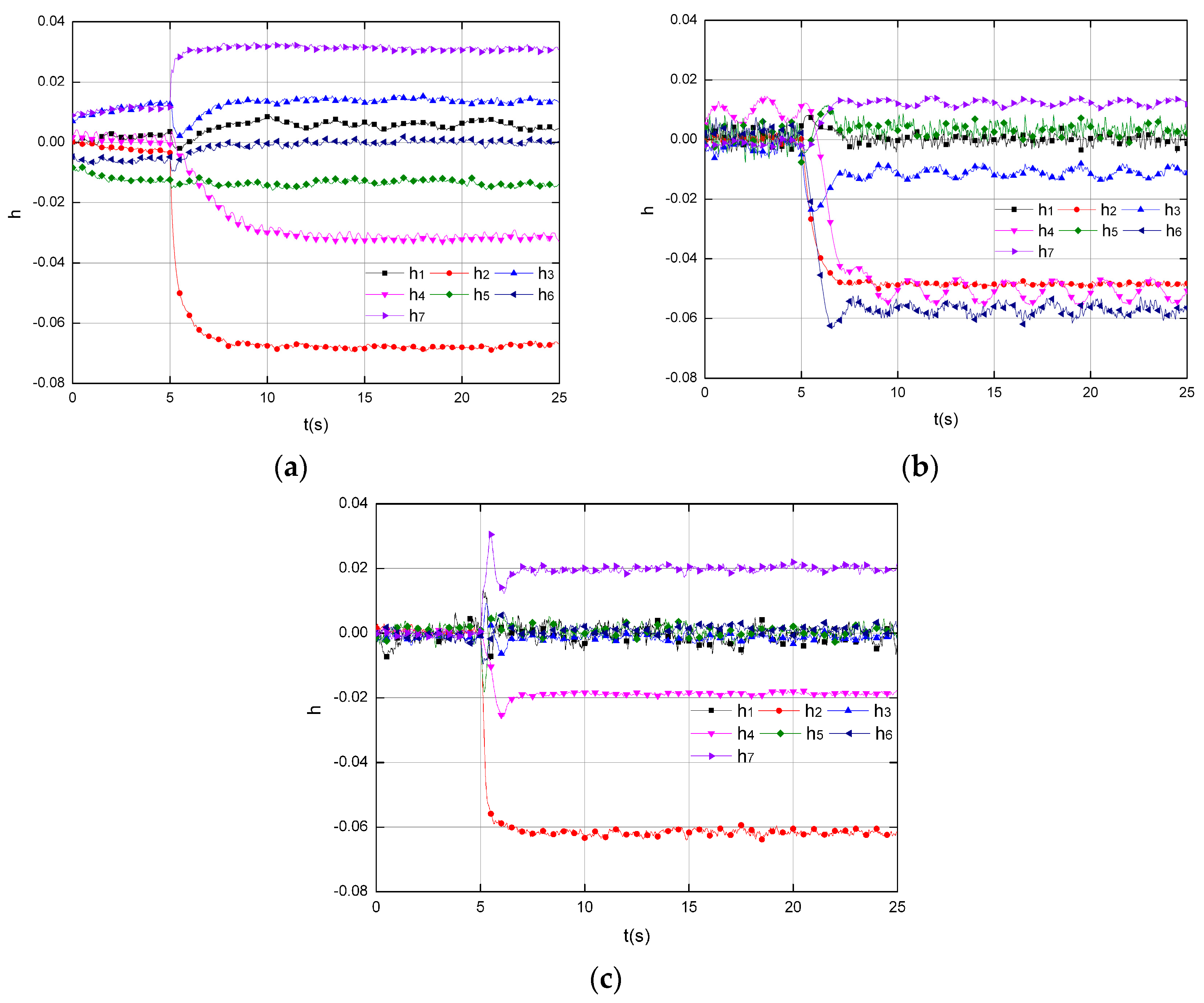
The simulations start with scenarios without uncertainty injections. Figure 4 depicts the health estimation by three tools, namely, the KF, the SMO in published work [25], and the SOSMO depicted in this paper, corresponding to the injected 8% decrease on $h_6$ that is applied at $t=5$ s (Mode 1). In Figure 4 all three tools are capable of health estimation under this circumstance, but their performance varies much. In Figure 4a, the KF performs with an acceptable accuracy, but the interval of the estimation process after the fault occurs (detection times) is about 7.85 s, which is the slowest reaction among three tools. Figure 4b depicts the estimation by the SMO, with a detecting time around 4.25 s, which is better than the KF. However, the chattering problem is evident, which may cause inaccurate estimation. Another problem is several healthy parameters ($h_3$ and $h_7$) decrease below 98% during estimation dynamics, and it may lead to misdiagnoses and false alarm. Finally Figure 4c shows the results conducted by SOSMO, with a desired accuracy and detection times. Compared to the first two tools, the SOSMO reacts much quicker, with the detection times about 1.05 s. Moreover, with super-twisting algorithm, the SOSMO performs better than SMO w.r.t the system chattering.

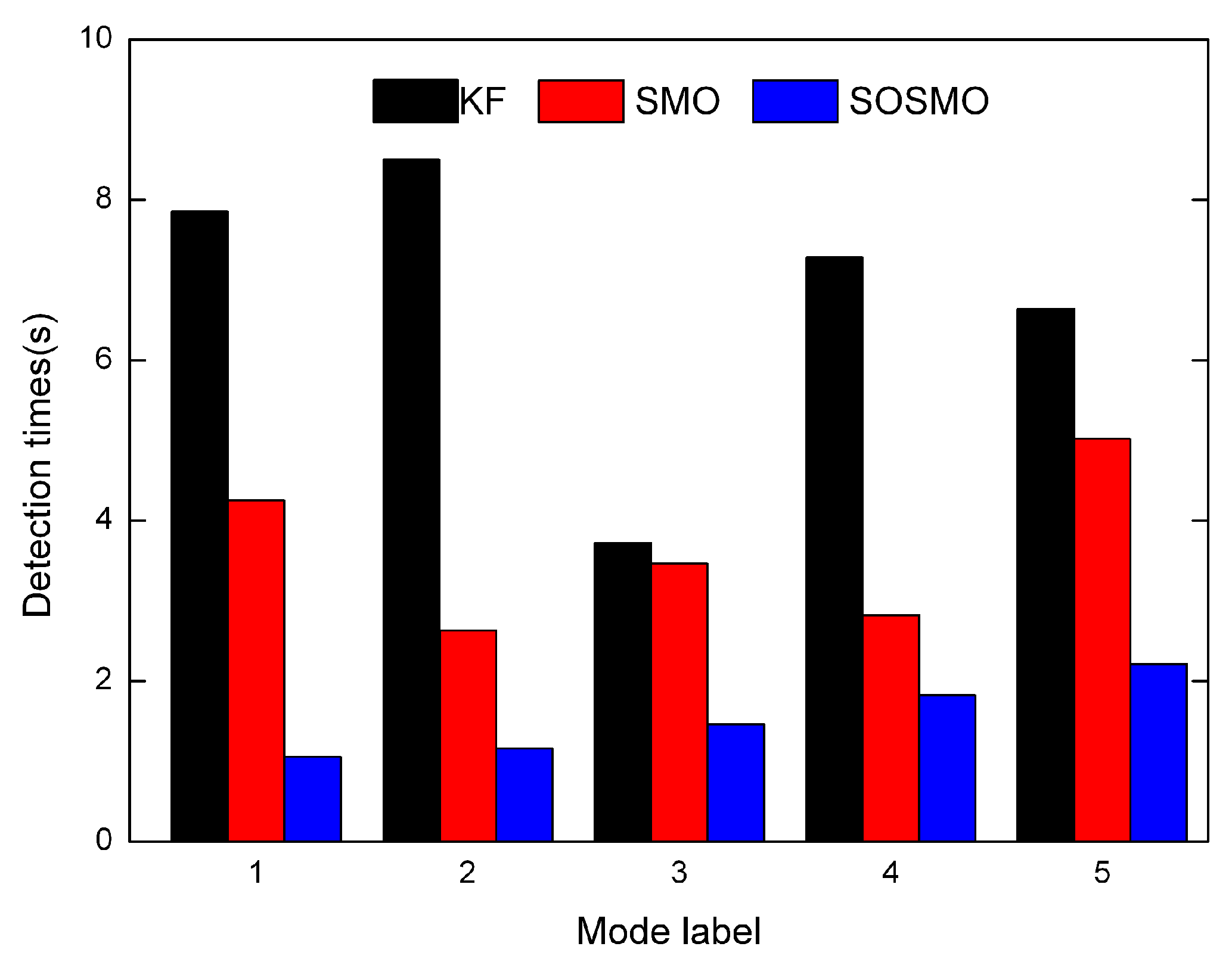
Figure 5 depicts the average detection times for each fault mode (Mode 1 to 5). It can be seen that the SOSMO consumes less time compared to the other two tools. This is because both the KF and the SMO work as state-estimator, and health parameters are modeled as state variables, the dynamics of which are assumed to be non-exist. That is to say the health parameters are expected to be slow evolving, which implies the KF and SMO schemes are not suitable for rapid fault cases. For SOSMO method, health parameters are modeled as unknown inputs, and the estimation is implemented by “fault reconstruction” concept. That means the SOSMO scheme have no limit on health parameters’ dynamics, which explains the ascendency of SOSMO in detection times.

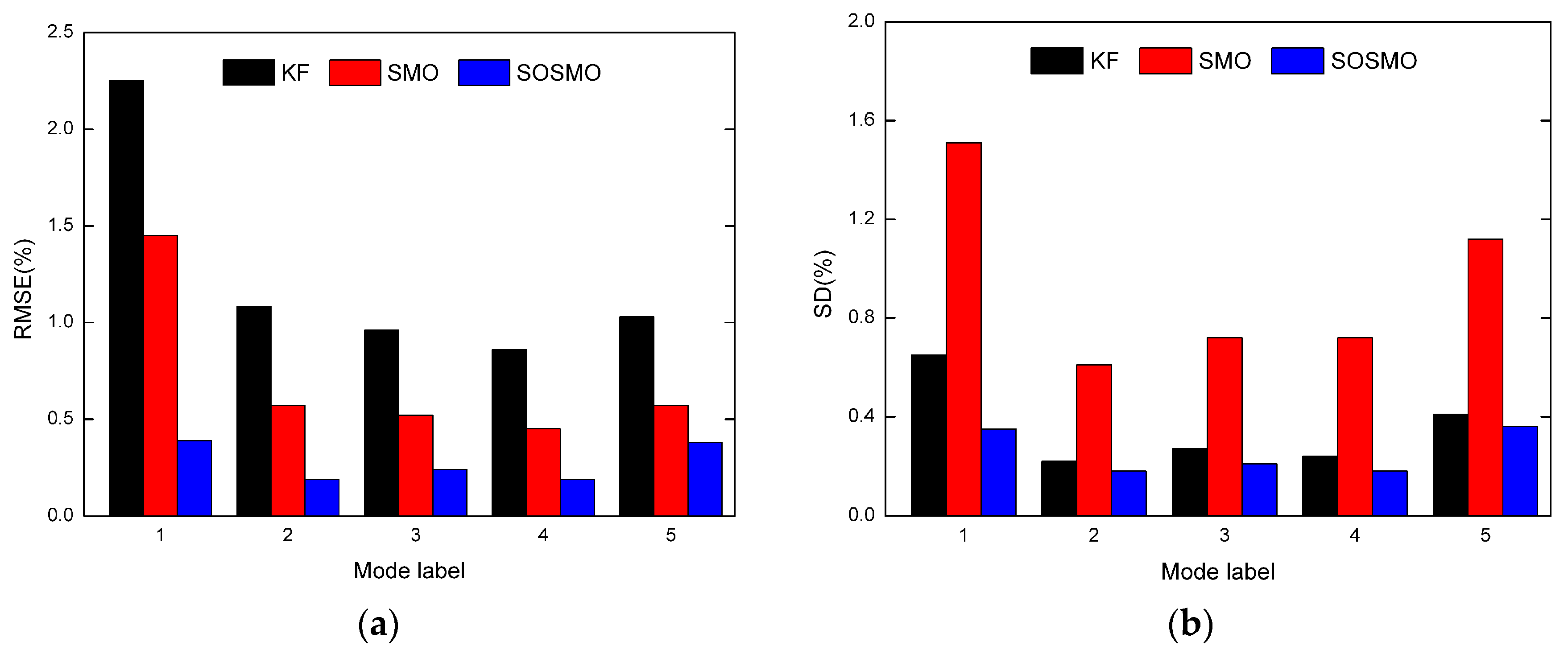
The accuracy of estimations performed by three tools is assessed in terms of the rooted square mean error (RSME) and the standard deviation (SD):

$$\begin{gathered} RMSE\left(m\right)=\sqrt{\frac{1}{D_f-D_s+1}{\displaystyle \sum }_{k=D_s}^{D_f}{\left({\widehat{h}}_k\left(m\right)-h_k\left(m\right)\right)}^2} \\ SD\left(m\right)=\sqrt{\frac{1}{D_f-D_s}{{\displaystyle \sum }}_{k=D_s}^{D_f}{\left({\widehat{h}}_k\left(m\right)-\frac{1}{D_f-D_s+1}{{\displaystyle \sum }}_{k=D_s}^{D_f}{\widehat{h}}_k\left(m\right)\right)}^2}, \end{gathered}$$

(42)

where $D_s$ and $D_f$ are the start point and the end point of the testing sequence, respectively. $h_k\left(m\right)$ is the $k\mathrm{th}$ value in the sequence of the mth health parameter, and ${\widehat{h}}_k\left(m\right)$ is its estimation value. From the definition, the RSME represents the precision of the estimation, while the SD reflects the dispersion degree. Figure 6 shows the statistics reflecting the averaged RSME and SD of seven health parameters in each fault mode. The RMSE results consistently imply the ascendency of the sliding mode observer in accuracy, while the SD results show the system chattering in sliding modes is well controlled to an acceptable level.

5.2. Scenarios with Uncertainties

When a linear observer/filter is used in GPHM scheme, one of the major concerns is the validity of the implemented tools subjected to model mismatches and system disturbances. The observer/filter may generate false estimation results in case of large uncertainties. However, by implementing the SOSMO in GPHM, uncertainties are automatically taken into account and become the prior optimized target. To demonstrate this advantage, in the next set of simulations, the performance of the proposed scheme is evaluated with modeling mismatches and disturbances injections. Similarly, the same problems conducted by the KF and SMO are also presented as comparison. Specify $\mathit{\xi }\left(\mathrm{t}\right)={\left[{\mathit{\xi }}_1\left(t\right),{\mathit{\xi }}_2\left(t\right)\right]}^{\mathrm{T}}$, where ${\mathit{\xi }}_1\left(t\right)\in {ℝ}^{1\times 1}$ denotes model mismatches, and ${\mathit{\xi }}_2\left(t\right)\in {ℝ}^{1\times 1}$ denotes disturbances. Assume that the model mismatches are in $\mathit{A}$ and $\mathit{C}$, then ${\mathit{\xi }}_1\left(t\right)$ is given by

$${\mathit{\xi }}_1\left(t\right)=\left[\begin{array}{ccc}\begin{array}{cc}\begin{array}{cc}\begin{array}{cc}0.2& 0.13\end{array}& \begin{array}{cc}0.11& 0.15\end{array}\end{array}& \begin{array}{cc}-0.4& -0.12\end{array}\end{array}& \begin{array}{cc}0.03& 0.54\end{array}& \begin{array}{cc}0.21& -0.14\end{array}\end{array}\right]{\mathit{x}}_a\left(t\right),$$

(43)

Further, a sine wave signal is employed to the state equation, to simulate disturbances on the actual engine, given by

$$\vartheta \left(t\right)=0.01+0.01sin\left(4\pi t\right),$$

(44)

Then by designating ${\mathit{\xi }}_2\left(t\right)=\left[\vartheta \left(t\right)\right]$, the uncertainty term in Equation (7) is attained by ${\mathit{Q}}_a\mathit{\xi }\left(\mathrm{t}\right)$, where ${\mathit{Q}}_a$ governs the distribution of $\mathit{\xi }\left(\mathrm{t}\right)$. The uncertainties modeled here are much different from that in [25]. The distribution matrix in [25] is strictly constrained to match a designed gain matrix, which is merely impractical in real application. In this work, although the choice of ${\mathit{Q}}_a$ has an influence on the reconstruction performance, there is no restriction on the structure or the value of ${\mathit{Q}}_a$, which is obviously more convincing.

Figure 7 depicts the results corresponding to the injected 6% decrease on $h_2$, 2% decrease on $h_4$ and 2% increase on $h_7$, that is applied at $t=5$ s (Mode 5). The results from Figure 7a,b are conducted by KF and SMO, separately. Due to the uncertainty injection, both two methods are failed to track the off-nominal parameters, and the normal ones are also wrongly estimated. This is because the uncertainty term is not covered in the design procedures of KF; meanwhile it does not follow the “matching condition” in SMO. In comparison, the results conducted by SOSMO are shown in Figure 7c, in which the health conditions are well tracked. Figure 8 shows the output errors in the estimation by three methods. In Figure 8b output errors in SMO never converge to 0, which means the sliding manifold is never arrived after the faults occur, and that explains the poor performance in Figure 7b. Figure 8c demonstrates the achievement of the output error convergence, and the sliding mode in SOSMO is attained soon after the faults occur, which is in accordance with the results in Figure 7c.

Again all considered abrupt fault modes (Mode 1 to 5) are examined by three tools in uncertainty-injection scenarios. Firstly the detection times in SOSMO scheme are investigated compared with the uncertainty-free cases.

Table 2. The detection times of SOSMO scheme in scenarios with uncertainties (s).

	Mode 1	Mode 2	Mode 3	Mode 4	Mode 5
With uncertainties	1.25	0.95	1.51	1.68	2.26
Without uncertainties	1.05	1.16	1.46	1.82	2.21

shows the results. The detection times are closed in both cases, which means they are not affected by the uncertainty injection. Then the estimating performance is evaluated in terms of the average RMSE and SD, shown in Figure 9a,b, respectively. From Figure 9a it’s evident that the SOSMO is significantly more robust to uncertainties than the other two tools, with a much better precision. Moreover, the SD results imply the chatting of SOSMO is on an acceptable level. The simulations demonstrate the ascendency of the proposed SOSMO scheme in health estimation problem considering uncertainties.

Considering engine parts wear from regular use, in the next simulation long-time degradation of is evaluated. The health parameters drift linearly away from the nominal values during flight cycles, and a rapid fault is imposed to the degraded health parameter, to check the effectiveness of observers/filters in real situations. The uncertainties are considered similarly, and the scenario simulated here is a rapid fault occurring during gradual degeneration, in which $h_2$ deteriorates to −4% of its nominal value in 5000 flight cycles (Mode 6). Figure 10a shows the estimating results conducted by SOSMO. The degraded parameters can be faithfully tracked, regardless of the slowness of degrading evolvement and the existence of disturbances, and the rapid fault occurred at 3000th cycle is detected and estimated accurately. By contrast, the KF scheme employed in the same condition produces poorer accuracy, as shown in Figure 10b, while SMO scheme produces higher chattering, as shown in Figure 10c. The average RMSE and SD results are shown in

Table 3. The average RMSE and SD corresponding to the injected 4% decrease on $h_2$ that is applied over 5000 cycles (Mode 6) in scenarios with uncertainties. (%)

	KF	SMO	SOSMO
RMSE	0.86	0.45	0.13
SD	0.38	0.44	0.28

, which again confirm and demonstrate the capability of the proposed SOSMO scheme in dealing with long-time degradation.

6. Conclusions

A second-order sliding mode observer based GPHM system for an aero-engine has been developed in this paper. Unlike the traditional state-estimator-based schemes, the proposed method estimates degradation via “unknown input reconstruction”. With health parameters modeled as artificial inputs, the described approach is applicable to both slow degradation and abrupt faults, and reacts much quicker than state-estimator-based schemes in abrupt fault cases. Considering the fact that the involved engine contains equal amount of available sensors and health parameters, instead of assuming “non-faulty sensors”, a transformation has been introduced to create a fictitious output that dimensionally outnumbers the health parameter vector, which makes the room for the robust design and meanwhile the diagnostic reliability is ensured. Then a second-order sliding mode observer has been described. The observer gains are synthesized by solving LMI problem, aiming at robustly estimating the degradation of health parameters, where the modeling mismatches and disturbances are considered. Also the high switching chattering is attenuated via the 2-order sliding mode methodology. A set of simulations have been conducted on the component-level model, and comparisons with the KF-based scheme and our previous SMO-based work have proven the ascendency of the proposed approach.