Comparison of Various Analysis Methods Based on Heat Flowmeters and Infrared Thermography Measurements for the Evaluation of the In Situ Thermal Transmittance of Opaque Exterior Walls


Abstract
1. Introduction
2. Evaluation Methods of -Value
2.1. Calculation Method
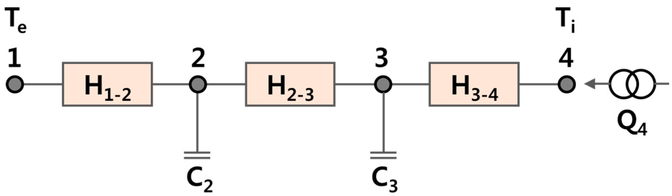
2.2. Heat Flowmeter Method
2.3. Infrared Thermography Method
3. In Situ Measurement of -Value
3.1. Investigated Buildings
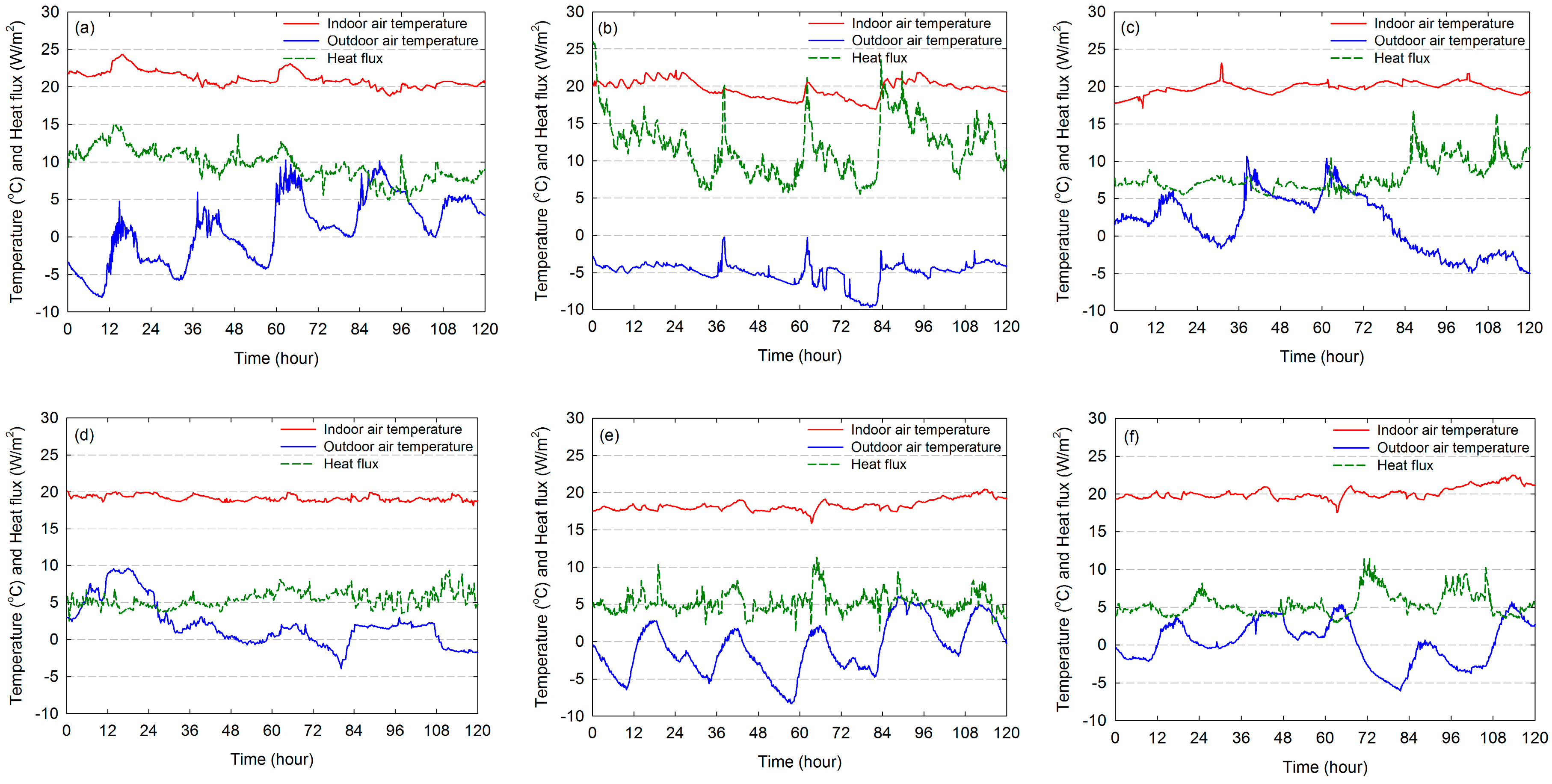
3.2. Measurement Procedure
4. Results and Analysis
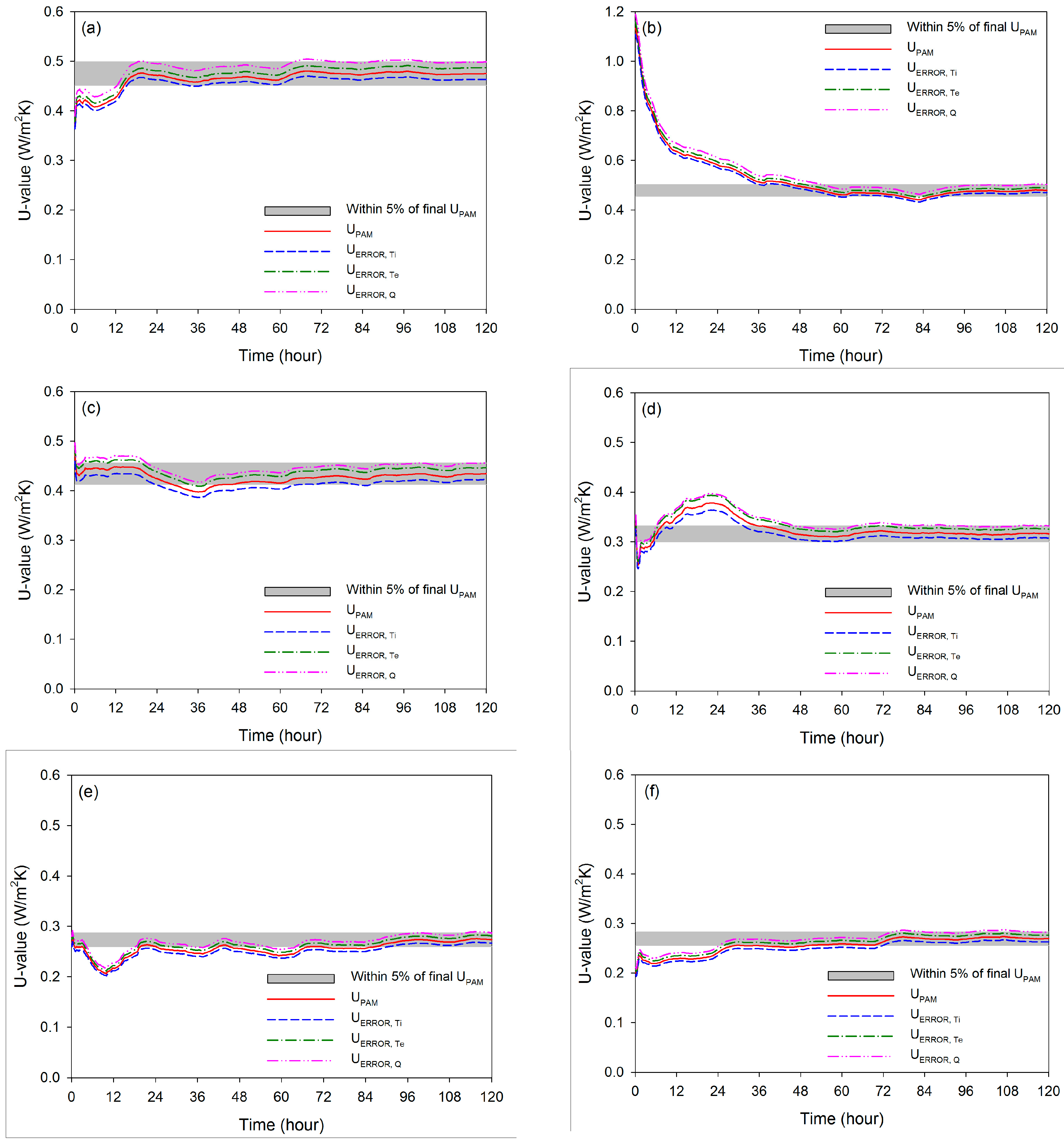
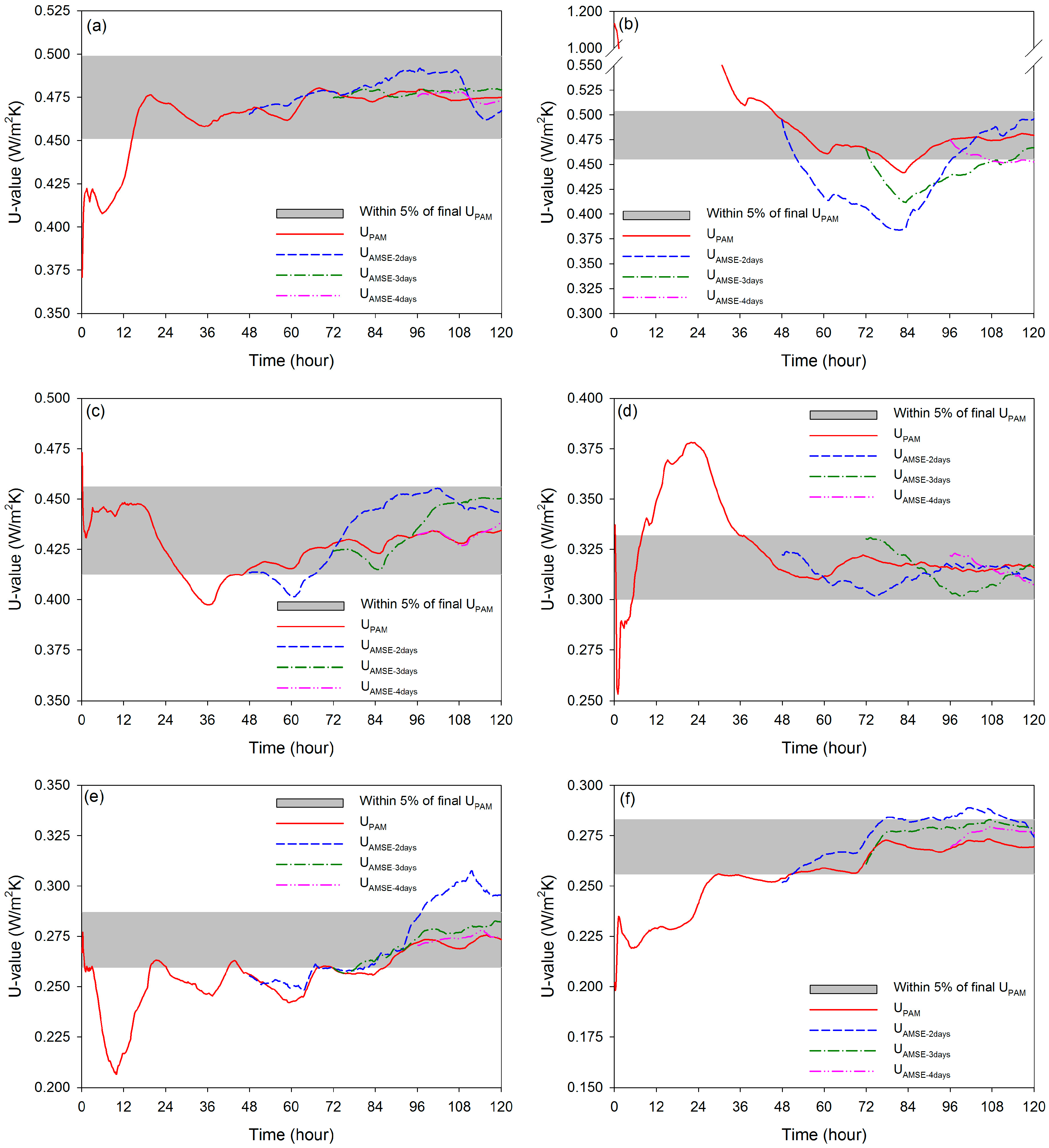
4.1. -Value Obtained with Progressive Average Method
4.2. -Value Corrected by Application of Thermal Storage Effect
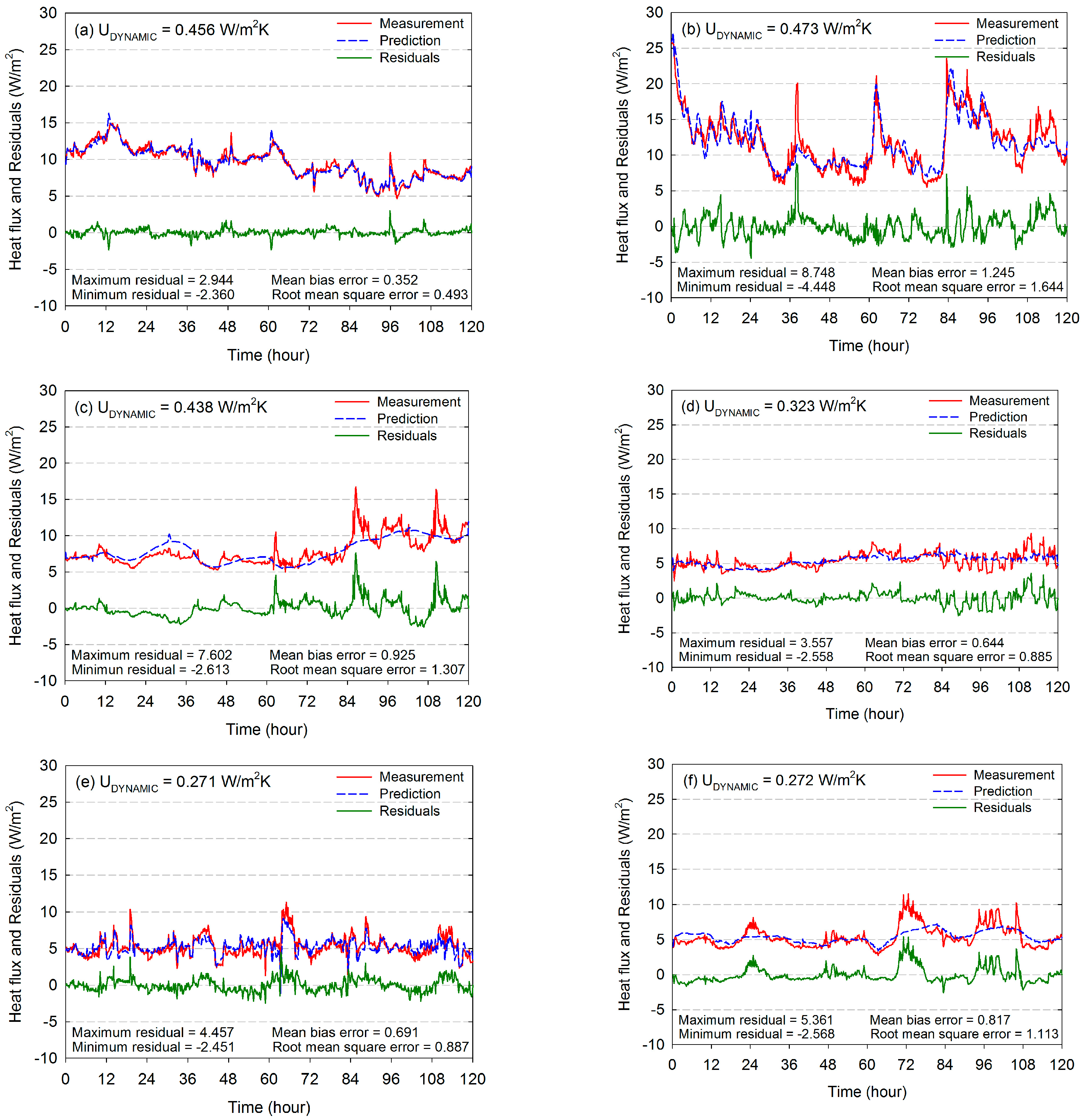
4.3. -Value Obtained with Dynamic Method
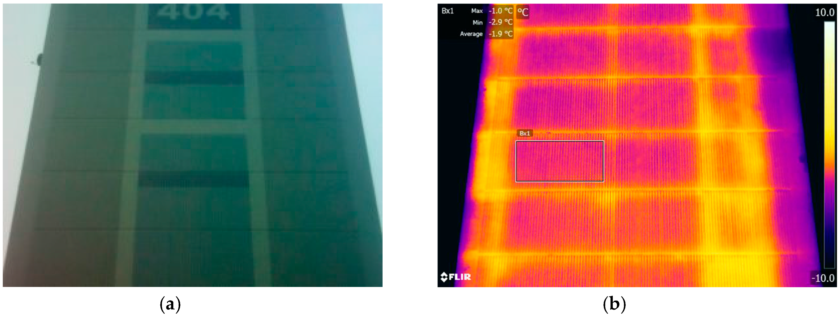
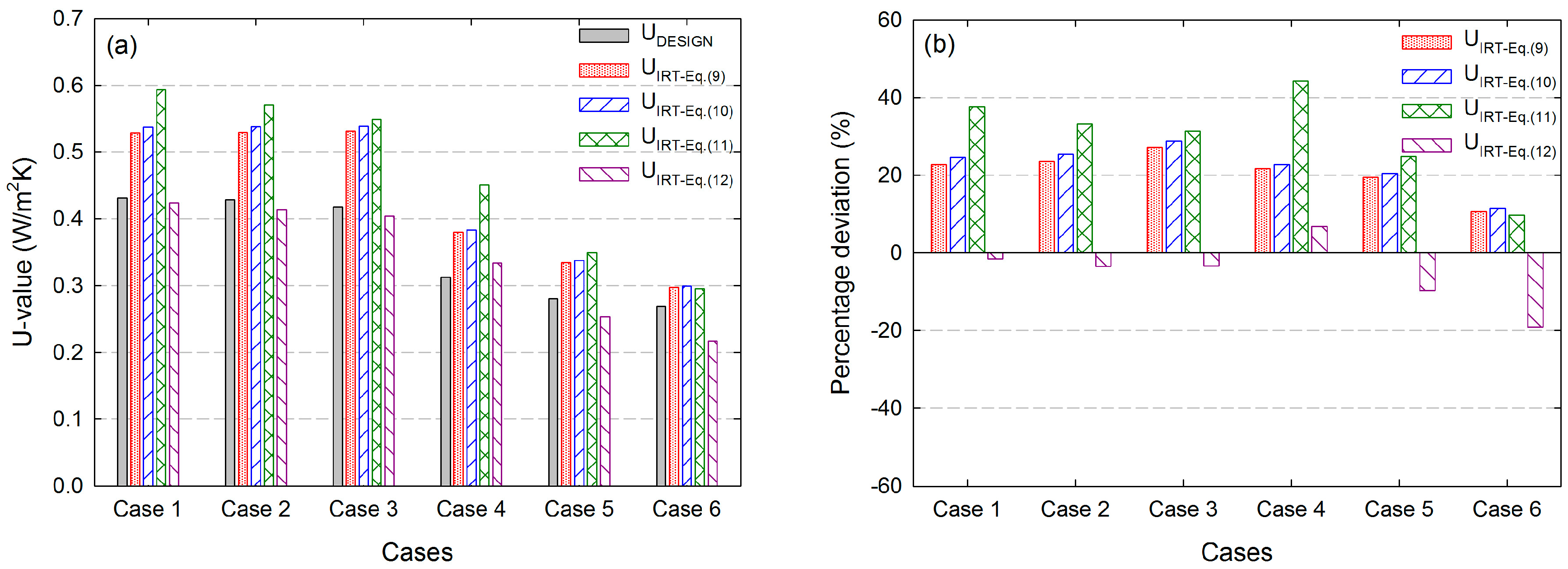
4.4. -Value Obtained with Infrared Thermography Method
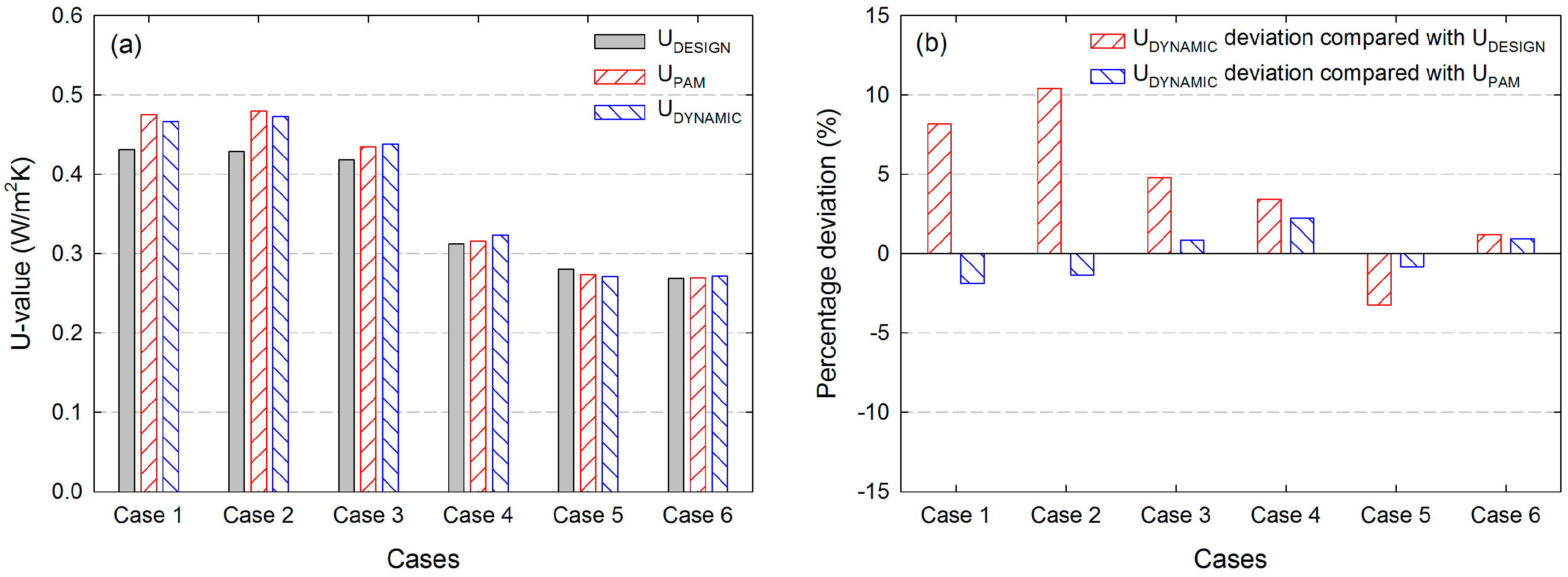
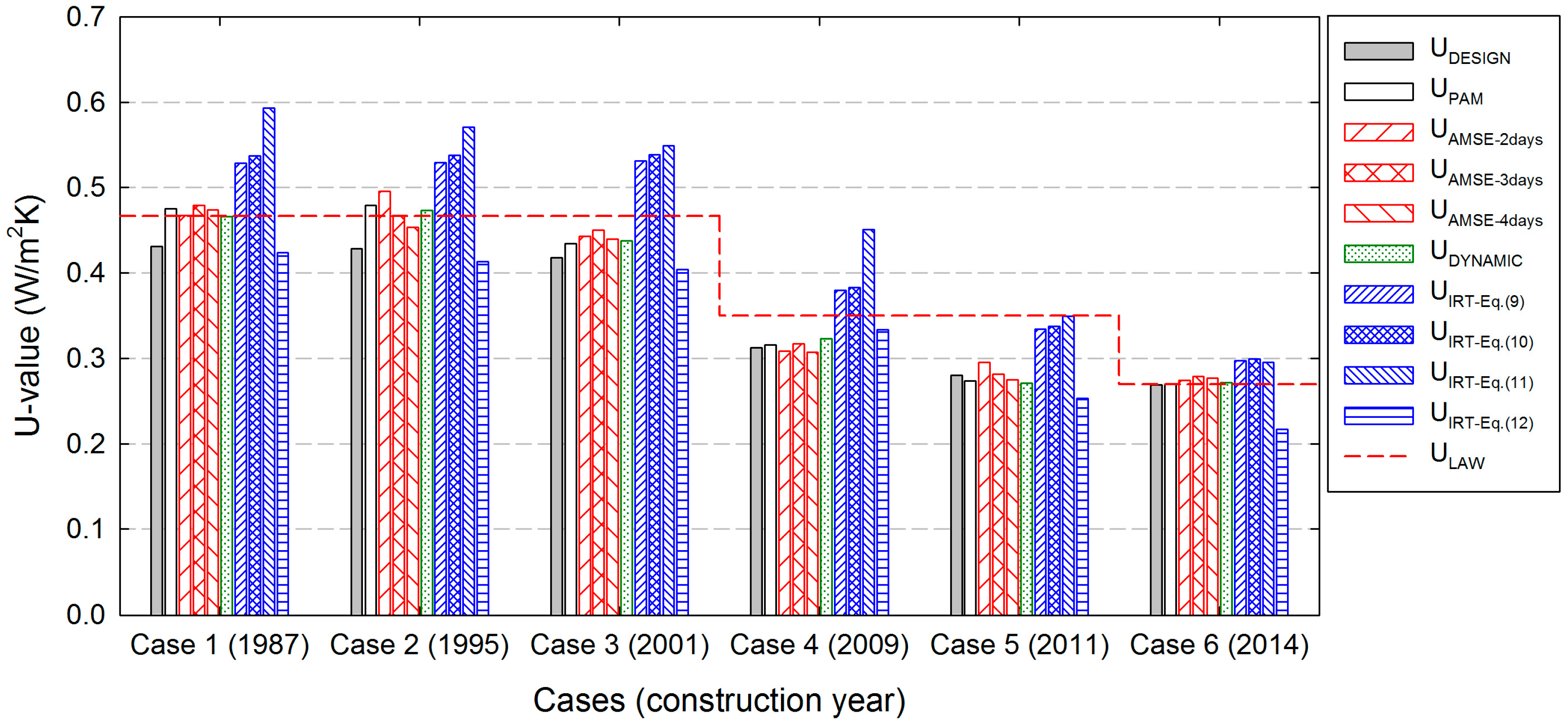
4.5. Comparison of Different -Value Evaluation Methods
5. Conclusions
Acknowledgments
Author Contributions
Conflicts of Interest
Nomenclature
| Thermal capacity of each layer, J/m2·K | |
| Material thickness, mm | |
| Exterior thermal mass correction factor, J/m2·K | |
| Interior thermal mass correction factor, J/m2·K | |
| Convective coefficient, W/m2·K | |
| The number of measurement data | |
| The number of layers that make up the wall | |
| Heat flux, W/m2 | |
| Sum of thermal resistances from the indoor environment to the k − 1th layer, m2·K/W | |
| Sum of thermal resistances from the k + 1th layer to the outdoor environment, m2·K/W | |
| Thermal resistance of each layer, m2·K/W | |
| Exterior surface resistance, m2·K/W | |
| Interior surface resistance, m2·K/W | |
| Total thermal resistance of the wall, m2·K/W | |
| Standard deviation of the thermal transmittance determined by the moving average method | |
| Exterior ambient temperature, K | |
| Interior ambient temperature, K | |
| Mean temperature between the exterior wall surface temperature and the reflected temperature, K | |
| Reflected temperature, K | |
| Exterior wall surface temperature, K | |
| Corrected thermal transmittance value taking into account the storage effect, W/m2·K | |
| Thermal transmittance evaluated by the calculation method, W/m2·K | |
| Thermal transmittance evaluated by the dynamic method, W/m2·K | |
| Thermal transmittance calculated by applying the heat flux sensor error, W/m2·K | |
| Thermal transmittance calculated by applying the interior temperature sensor error, W/m2·K | |
| Thermal transmittance calculated by applying the exterior temperature sensor error, W/m2·K | |
| Thermal transmittance evaluated by the infrared thermography method, W/m2·K | |
| Thermal transmittance evaluated by the progressive average method, W/m2·K | |
| Wind speed, m/s | |
| Difference between interior average temperature over 24 h prior to reading j and interior average temperature over the first 24 h of the analysis period, K | |
| Difference between exterior average temperature over 24 h prior to reading j and exterior average temperature over the first 24 h of the analysis period, K | |
| Interior temperature sensor error, K | |
| Overall uncertainty in the thermal transmittance evaluation, W/m2·K | |
| Thermal emissivity across the entire spectrum | |
| Thermal emissivity in the wavelength range of the infrared camera | |
| Thermal conductivity, W/m·K | |
| Stefan-Boltzmann constant | |
| Interval between readings, s |
References and Note
- Nardi, I.; Paoletti, D.; Ambrosini, D.; Rubeis, T.D.; Sfarra, S. Validation of quantitative IR thermography for estimating the U-value by a hot box apparatus. In Proceedings of the 33th UIT (Italian Union of Thermo-Fluid-Dynamics) Heat Transfer Conference, L’Aquila, Italy, 22–24 June 2015. [Google Scholar]
- Albatici, R.; Passerini, F.; Tonelli, A.M.; Gialanella, S. Assessment of the Thermal Emissivity Value of Building Materials Using an Infrared Thermovision Technique Emissometer. Energy Build. 2013, 66, 33–40. [Google Scholar] [CrossRef]
- ISO 9869–1:2014. Building elements—in-situ measurement of thermal resistance and thermal transmittance—Part 1: Heat flow meter method. Available online: https://www.iso.org/standard/59697.html (accessed on 13 July 2017).
- Danielski, I.; Fröling, M. Diagnosis of buildings’ thermal performance—A quantitative method using thermography under non-steady state heat flow. Energy Procedia 2015, 83, 320–329. [Google Scholar] [CrossRef]
- Adhikari, R.S.; Lucchi, E.; Pracchi, V. Experimental measurements on thermal transmittance of the opaque vertical walls in the historical buildings. In Proceedings of the 28th International PLEA Conference on Sustainable Architecture + Urban Design, Lima, Peru, 7–9 November 2012. [Google Scholar]
- Asdrubali, F.; D’Alessandro, F.; Baldinelli, G.; Bianchi, F. Evaluating in situ thermal transmittance of green buildings masonries—A case study. Case Stud. Constr. Mater. 2014, 1, 53–59. [Google Scholar] [CrossRef]
- Cesaratto, P.G.; Carli, M.D. A measuring campaign of thermal conductance in situ and possible impacts on net energy demand in buildings. Energy Build. 2013, 59, 29–36. [Google Scholar] [CrossRef]
- Meng, X.; Yan, B.; Gao, Y.; Wang, J.; Zhang, W.; Long, E. Factors affecting the in situ measurement accuracy of the wall heat transfer coefficient using the heat flow meter method. Energy Build. 2015, 86, 754–765. [Google Scholar] [CrossRef]
- Peng, C.; Wu, Z. In situ measuring and evaluating the thermal resistance of building construction. Energy Build. 2008, 40, 2076–2082. [Google Scholar] [CrossRef]
- Evangelisti, L.; Guattari, C.; Gori, P.; Vollaro, R.D.L. In situ thermal transmittance measurements for investigating differences between wall models and actual building performance. Sustainability 2015, 7, 10388–10398. [Google Scholar] [CrossRef]
- Kylili, A.; Focaides, P.A.; Christou, P.; Kalogirou, S.A. Infrared thermography (IRT) applications for building diagnostics: A review. Appl. Energy 2014, 134, 531–549. [Google Scholar] [CrossRef]
- Haralambopoulos, D.A.; Paparsenos, G.F. Assessing the thermal insulation of old buildings—The need for in situ spot measurements of thermal resistance and planar infrared thermography. Energy Convers. Manag. 1998, 39, 65–79. [Google Scholar] [CrossRef]
- Balaras, C.A.; Argiriou, A.A. Infrared thermography for building diagnostics. Energy Build. 2002, 34, 171–183. [Google Scholar] [CrossRef]
- Ocana, S.M.; Guerrero, I.C.; Requena, I.G. Thermographic survey of two rural buildings in Spain. Energy Build. 2004, 36, 515–523. [Google Scholar] [CrossRef]
- Kalamees, T. Air tightness and air leakages of new lightweight single-family detached houses in Estonia. Build. Environ. 2007, 42, 2369–2377. [Google Scholar] [CrossRef]
- Taylor, T.; Counsell, J.; Gill, S. Energy efficiency is more than skin deep: Improving construction quality control in new-build housing using thermography. Energy Build. 2013, 66, 222–231. [Google Scholar] [CrossRef]
- Albatici, R.; Tonelli, A.M. Infrared thermovision technique for the assessment of the thermal transmittance value of opaque building elements on site. Energy Build. 2010, 42, 2177–2183. [Google Scholar] [CrossRef]
- Albatici, R.; Tonelli, A.M.; Chiogna, M. A comprehensive experimental approach for the validation of quantitative infrared thermography in the evaluation of building thermal transmittance. Appl. Energy 2015, 141, 218–228. [Google Scholar] [CrossRef]
- Fokaides, P.A.; Kalogirou, S.A. Application of infrared thermography for the determination of the overall heat transfer coefficient (U-Value) in building envelopes. Appl. Energy 2011, 88, 4358–4365. [Google Scholar] [CrossRef]
- Dall’O’, G.; Sarto, L.; Panza, A. Infrared screening of residential buildings for energy audit purposes: Results of a field test. Energies 2013, 6, 3859–3878. [Google Scholar] [CrossRef]
- Nardi, I.; Sfarra, S.; Ambrosini, D. Quantitative thermography for the estimation of the U-value: state of the art and a case study. In Proceedings of the 32nd UIT (Italian Union of Thermo-fluid-dynamics) Heat Transfer Conference, Pisa, Italy, 23–25 June 2014. [Google Scholar]
- Nardi, I.; Ambrosini, D.; Rubeis, T.D.; Sfarra, S.; Perilli, S.; Pasqualoni, G. A comparison between thermographic and flow-meter methods for the evaluation of thermal transmittance of different wall constructions. In Proceedings of the 33th UIT (Italian Union of Thermo-fluid-dynamics) Heat Transfer Conference, L’Aquila, Italy, 22–24 June 2015. [Google Scholar]
- ISO 6946: 2007. Building Components and Building Elements—Thermal Resistance and Thermal Transmittance—Calculation Method. Available online: https://www.iso.org/standard/40968.html (accessed on 13 July 2017).
- Simões, I.; Simões, N.; Tadeu, A.; Riachos, J. Laboratory assessment of thermal transmittance of homogeneous building elements using infrared thermography. In Proceedings of the 12th International Conference on Quantitative InfraRed Thermography, Bordeaux, France, 7–12 July 2014. [Google Scholar]
- Rhee-Duverne, S.; Baker, P. Research into the Thermal Performance of Traditional Brick Walls. 2013. Available online: https://content.historicengland.org.uk/images-books/publications/thermal-performance-traditional-windows-summary/sash-windows-research-summary.pdf/ (accessed on 30 June 2017).
- DYNamic Analysis, Simulation and Testing Applied to the Energy and Environmental Performance of Buildings (DYNASTEE). Available online: http://dynastee.info/data-analysis/software-tools/lord (accessed on 30 June 2017).
- LORD 3.2. Available online: http://dynastee.info/wp-content/uploads/2012/12/lordmanual.pdf (accessed on 30 June 2017).
- Gutschker, O. Parameter identification with the software package LORD. Build. Environ. 2008, 43, 163–169. [Google Scholar] [CrossRef]
- Madding, R. Finding R-values of stud frame constructed houses with IR thermography. In Proceedings of the InfraMation, Reno, NV, USA, 3–7 November 2008; pp. 261–277. [Google Scholar]
- Watanabe, K. Architectural Planning Fundamentals. 1965. [Google Scholar]
- ASTM C 680—14. Standard Practice for Estimate of the Heat Gain or Loss and the Surface Temperatures of Insulated Flat, Cylindrical, and Spherical Systems by Use of Computer Programs. Available online: https://www.astm.org/Standards/C680.htm (accessed on 13 July 2017).
- Nardi, I.; Paoletti, D.; Ambrosini, D.; Rubeis, T.D.; Sfarra, S. U-value assessment by infrared thermography: A comparison of different calculation methods in a Guarded Hot Box. Energy Build. 2016, 122, 211–221. [Google Scholar] [CrossRef]
- ASTM E 1862-97. Standard Test Methods for Measuring and Compensating for Reflected Temperature Using Infrared Imaging Radiometers. Available online: http://www.irss.ca/development/documents/CODES%20&%20STANDARDS_02-28-08/ASTM/Thermography/Test%20Method%20for/E1862-97%20Infrared%20Imaging%20Radiometers.pdf (accessed on 13 July 2017).
- ASTM E 1933-99a. Standard Test Methods for Measuring and Compensating for Emissivity Using Infrared Imaging Radiometers. Available online: https://www.astm.org/DATABASE.CART/HISTORICAL/E1933-99A.htm (accessed on 13 July 2017).
- Strachan, P.A.; Vandaele, L. Case studies of outdoor testing and analysis of building components. Build. Environ. 2008, 43, 129–142. [Google Scholar] [CrossRef]
- Baker, P.H.; Dijk, H.A.L. PASLINK and dynamic outdoor testing of building components. Build. Environ. 2008, 43, 143–151. [Google Scholar] [CrossRef]


| Cases | On-site Photo (Permission Year/Construction Year) | Material Layer | d (mm) | (W/m·K) | R (m2·K/W) | (W/m2·K) |
|---|---|---|---|---|---|---|
| Case 1 |  (1985/1987) | Internal surface | 0.110 | 0.431 | ||
| Gypsum board | 10 | 0.180 | 0.056 | |||
| Glass wool | 70 | 0.035 | 2.000 | |||
| Concrete | 180 | 1.600 | 0.113 | |||
| External surface | 0.043 | |||||
| Case 2 |  (1993/1995) | Internal surface | 0.110 | 0.429 | ||
| Gypsum board | 10 | 0.180 | 0.056 | |||
| Glass wool | 70 | 0.035 | 2.000 | |||
| Concrete | 200 | 1.600 | 0.125 | |||
| External surface | 0.043 | |||||
| Case 3 |  (1999/2001) | Internal surface | 0.110 | 0.418 | ||
| Gypsum board | 10 | 0.180 | 0.056 | |||
| Expanded polystyrene | 70 | 0.034 | 2.059 | |||
| Concrete | 200 | 1.600 | 0.125 | |||
| External surface | 0.043 | |||||
| Case 4 |  (2007/2009) | Internal surface | 0.110 | 0.312 | ||
| Gypsum board | 12 | 0.180 | 0.067 | |||
| Glass wool | 100 | 0.035 | 2.857 | |||
| Concrete | 200 | 1.600 | 0.125 | |||
| External surface | 0.043 | |||||
| Case 5 |  (2009/2011) | Internal surface | 0.110 | 0.280 | ||
| Gypsum board | 12 | 0.180 | 0.067 | |||
| Expanded polystyrene | 100 | 0.031 | 3.226 | |||
| Concrete | 200 | 1.600 | 0.125 | |||
| External surface | 0.043 | |||||
| Case 6 |  (2012/2014) | Internal surface | 0.110 | 0.269 | ||
| Gypsum board | 10 | 0.180 | 0.056 | |||
| Expanded polystyrene | 105 | 0.031 | 3.387 | |||
| Concrete | 200 | 1.600 | 0.125 | |||
| External surface | 0.043 |
| Cases | Construction Year | (W/m2·K) | (W/m2·K) | Deviation Compared to (%) | Deviation during Test (%) | Uncertainty of | ||
|---|---|---|---|---|---|---|---|---|
| 24 h before End of Test | INT(2DT/3)d before End of Test | (W/m2·K) | Overall Uncertainty (%) | |||||
| Case 1 | 1987 | 0.431 | 0.475 | 10.25 | 0.86 | −1.49 | 0.033 | 6.98 |
| Case 2 | 1995 | 0.429 | 0.479 | 11.89 | −0.94 | 3.25 | 0.071 | 14.75 |
| Case 3 | 2001 | 0.418 | 0.434 | 3.92 | −0.48 | −4.34 | 0.037 | 8.43 |
| Case 4 | 2009 | 0.312 | 0.316 | 1.15 | −0.18 | −0.49 | 0.025 | 7.85 |
| Case 5 | 2011 | 0.280 | 0.273 | −2.42 | −0.48 | −6.38 | 0.035 | 12.66 |
| Case 6 | 2014 | 0.269 | 0.269 | 0.26 | −0.27 | −5.80 | 0.021 | 7.93 |
| Cases | Construction Year | (W/m2·K) | for Different Analysis Periods (W/m2·K) | Deviation Compared with (%) | ||||
|---|---|---|---|---|---|---|---|---|
| Case 1 | 1987 | 0.431 | 0.467 | 0.479 | 0.474 | 8.44 | 11.26 | 10.02 |
| Case 2 | 1995 | 0.429 | 0.496 | 0.467 | 0.453 | 15.70 | 8.92 | 5.79 |
| Case 3 | 2001 | 0.418 | 0.443 | 0.450 | 0.440 | 5.99 | 7.72 | 5.25 |
| Case 4 | 2009 | 0.312 | 0.309 | 0.317 | 0.307 | −1.20 | 1.47 | −1.65 |
| Case 5 | 2011 | 0.280 | 0.295 | 0.282 | 0.275 | 5.50 | 0.65 | −1.90 |
| Case 6 | 2014 | 0.269 | 0.274 | 0.279 | 0.277 | 2.07 | 3.65 | 2.93 |
| Cases | Construction Year | (W/m2·K) | Tse (°C) | Te (°C) | Ti (°C) | Tref (°C) | Tm (°C) | (-) | Ve (m/s) | (W/m2·K) | |||
|---|---|---|---|---|---|---|---|---|---|---|---|---|---|
| Equation (9) | Equation (10) | Equation (11) | Equation (12) | ||||||||||
| Case 1 | 1987 | 0.431 | −2.00 | −4.50 | 21.87 | −5.20 | −3.55 | 0.90 | 0.12 | 0.529 | 0.537 | 0.593 | 0.424 |
| Case 2 | 1995 | 0.429 | −1.90 | −4.25 | 21.66 | −5.00 | −3.48 | 0.91 | 0.13 | 0.529 | 0.538 | 0.571 | 0.414 |
| Case 3 | 2001 | 0.418 | 0.80 | −1.14 | 20.30 | −1.80 | −0.51 | 0.91 | 0.07 | 0.531 | 0.539 | 0.549 | 0.404 |
| Case 4 | 2009 | 0.312 | 0.60 | −0.78 | 18.62 | −1.00 | −0.25 | 0.90 | 0.14 | 0.380 | 0.383 | 0.450 | 0.334 |
| Case 5 | 2011 | 0.280 | −1.90 | −3.08 | 17.78 | −3.50 | −2.76 | 0.91 | 0.10 | 0.334 | 0.337 | 0.350 | 0.253 |
| Case 6 | 2014 | 0.269 | −0.70 | −1.68 | 19.61 | −2.10 | −1.42 | 0.90 | 0.16 | 0.297 | 0.299 | 0.295 | 0.217 |
© 2017 by the authors. Licensee MDPI, Basel, Switzerland. This article is an open access article distributed under the terms and conditions of the Creative Commons Attribution (CC BY) license (http://creativecommons.org/licenses/by/4.0/).
Share and Cite
Choi, D.S.; Ko, M.J. Comparison of Various Analysis Methods Based on Heat Flowmeters and Infrared Thermography Measurements for the Evaluation of the In Situ Thermal Transmittance of Opaque Exterior Walls. Energies 2017, 10, 1019. https://doi.org/10.3390/en10071019
Choi DS, Ko MJ. Comparison of Various Analysis Methods Based on Heat Flowmeters and Infrared Thermography Measurements for the Evaluation of the In Situ Thermal Transmittance of Opaque Exterior Walls. Energies. 2017; 10(7):1019. https://doi.org/10.3390/en10071019
Chicago/Turabian StyleChoi, Doo Sung, and Myeong Jin Ko. 2017. "Comparison of Various Analysis Methods Based on Heat Flowmeters and Infrared Thermography Measurements for the Evaluation of the In Situ Thermal Transmittance of Opaque Exterior Walls" Energies 10, no. 7: 1019. https://doi.org/10.3390/en10071019
APA StyleChoi, D. S., & Ko, M. J. (2017). Comparison of Various Analysis Methods Based on Heat Flowmeters and Infrared Thermography Measurements for the Evaluation of the In Situ Thermal Transmittance of Opaque Exterior Walls. Energies, 10(7), 1019. https://doi.org/10.3390/en10071019