Finite Element Computation of Transient Parameters of a Salient-Pole Synchronous Machine

Abstract

This paper presents a novel method for calculating the transient parameters of a saturated salient-pole synchronous machine (SPSM) with damper cage using finite element analysis. All detailed leakage inductances in a modified d-q model are discussed and separately extracted. In addition; the frozen permeability method is used in a 2-D finite element analysis to consider saturation and skin effects for determining the inductances. The terminal reactance parameters are obtained from all elements of the d- and q-axis equivalent circuits in all the chosen time constants during the transient process. The variation of leakage inductances of the SPSM in transient processes is also investigated and discussed. To determine transient time constant parameters; the Prony algorithm is applied in the presented method. A program developed to automatically solve the simulation and computation with the proposed method is described. This method is applied to a prototype and validated by experimental results. Some discussion about the relationship between rotor geometric design and the transient parameters of SPSMs is provided. The variation of leakage magnetic field of SPSMs in transient processes is also investigated. This method can be applied in transient parameter estimation and optimization of SPSMs in the design stage.

1. Introduction

Transient parameters of electrical machines are generally applied to estimate the dynamic behavior of machines in power system analysis [1,2]. The salient-pole synchronous machine (SPSM) is one of the most-used types of machine in industrial application. In hydroelectric plants, SPSMs have been applied as generators since the nineteenth century. The SPSM is also preferred as the type of generator used in ships [3]. In traction drive, mine hoist, and marine propulsion, SPSMs are commonly employed as drive motors [4]. Besides, SPSMs have a long history of utilization as motor-generators in pumped storage plants and as synchronous compensators in some substations. As most of the SPSMs are connected with the power grid, accurate calculation of the transient parameters is critical in determining the dynamic performance of a SPSM.

In the literature, there are many reports of various tests and methods to estimate the transient parameters of a synchronous machine, which are represented as terminal operational impedances and time constants [5,6]. However, these studies mainly focus on a machine that has already been designed or produced. In the design stage, precise determination of the transient parameters of an SPSM is also important for refinement. The designers not only concentrate on the terminal parameters, but also prefer to accurately calculate each element of the magnetic equivalent circuit for design optimization.

The analytical solution is traditionally applied in machine design to calculate the transient parameters from the equivalent circuit and lumped parameter model [7,8]. However, the accuracy of analytical formulas is inadequate due to the simplified assumptions and many correction factors made in the calculation procedure. The finite element (FE) method has been recently applied in various SPSM analyses [9,10], which makes the consideration of saturation and skin effects come true. By employing FE analysis, the accuracy of computation, compared with analytical solution, is significantly improved. For example, the standard three-phase sudden short-circuit test is simulated in [9], and the standstill frequency response test is simulated in [10] by using a time-stepping FE analysis to obtain terminal transient parameters.

Though several studies about transient parameter calculation by the FE method have been reported, the existing methods do not fully satisfy the demands of designers. In the traditional method given in [11] and applied in [9], transient parameters are obtained from short-circuit current waveform by wave analysis. This method is relatively subjective, and only suitable for terminal parameters’ computation. For FE simulations of standstill frequency response tests [10], it is hard to follow the same magnetization saturation effects in the dynamic process, which would influence the accuracy of parameters obtained by these methods. In [12], an improved curve-fitting method based on the Levenberg–Marquardt algorithm is proposed. This method is more suitable for small machines and overcomes some drawbacks of the traditional method like subjectivity. However, the detailed magnetic equivalent circuit parameters needed by designers can’t be extracted in this method. Besides, the influence of inductance variation during dynamic processes on transient parameters is not considered and represented in the afore-mentioned methods.

For designers, a novel computational method that can produce more detailed information is needed for the computation of the transient parameters of an SPSM. Several demands of the required method are as follows. The inductance parameters and the time constants are expected to be calculated directly and automatically by FE analysis. The detailed inductance parameters of the magnetic equivalent circuit should be extracted separately for design optimization. And the inductance variation during dynamic processes ought to be considered in the computation.

Accurate computation of magnetic equivalent circuit parameters using FE analysis is an important part of inductance calculation in the novel method. A lot of related work has been previously reported in the literature [13,14,15,16,17]. Magnetic vector potential (MVP) methods have been used to calculate the inductance parameters [13]. In addition, the frozen permeability method was applied in [14] to consider the core saturation and skin effect of the solid conductor bar. A detailed SPSM leakage inductance model has been generated that considers the leakage flux distribution flowing across the air gap [15,16,17]. In the literature [16,17], the influence of various operational statuses on leakage inductance variation is discussed, and the leakage inductances are obtained at the steady state FE simulation. But, the magnetic field distribution of an SPSM in transient process is time varying and different from steady state as investigated in this paper. This phenomenon should also be considered in the computational analysis of leakage inductance and finally in the determination of transient parameters. FE computation of leakage inductances has been previously reported and discussed in [14,15,16,17,18,19]. For time constant determination, a curve fitting technique might be helpful when applied to calculate the time constants [12,20].

Basing on the previous works mentioned above, a novel method for transient parameters computation of an SPSM in the design stage is proposed in this paper. In this method, time-stepping field-circuit FE simulation and static magnetic FE simulation are employed for accurate calculation. All elements of equivalent circuit parameters can be separately extracted by this method. In particular, the gap leakage inductances [15] are considered and obtained. The inductance variation, influenced by saturation variation during the whole transient process, are investigated and considered in the determination of transient parameters. To estimate time constants, the Prony algorithm is applied. The proposed method satisfies the afore-mentioned demand of SPSM designers. Besides, a program is developed to control the FE simulation and data processing [21]. By employing this program, the transient parameters can be automatically calculated in the proposed method.

The rest of this paper is organized as follows. Section 2 discusses the modification of the d-q model of an SPSM, which considers the leakage inductances separately and presents the equivalent circuits for calculating the transient parameters. The calculation procedure using a 2-D FE analysis of a three-phase sudden short-circuit test simulation is described in Section 3; the procedure includes the method to obtain the magnetic equivalent circuit parameters separately considering the saturation variation and skin effects, and the method to compute the transient parameters. Section 4 and Section 5 provide the results, discussion, method validation, and conclusion.

2. Machine Model

The d-q model describes an SPSM with damper cage whose stator core and rotor pole are both laminated. A cross-section schematic of the SPSM is shown in Figure 1.

2.1. Damper Cage Model

A damper cage with inter-pole connections is modeled by the multi-loop method in [15] as a multi-loop model having N_d and N_q windings along the d- and q-axes, respectively. However, this method is too complex to obtain the integral characteristics of the damper cage in practical applications. In this paper, the damper cage is modeled as two concentric windings, kD and kQ, along the d- and q-axes, respectively. kD and kQ consist of N_d and N_q concentrated coils, respectively. The turn numbers (TN) of each coil are adjusted to keep the magnetic motive force (MMF) of kD and kQ equal to the sum of the MMF of the multi-loop model windings along the d- and q-axes, as shown in Equations (1) and (2).

$$\begin{array}{r}{\mathrm{TN}}_{iD}=\frac{I_{id}}{I_{kD}}\begin{array}{cc}& (i=2,\dots ,N_d)\end{array}\begin{array}{cc},& {\mathrm{TN}}_{N_{d}D}=1\end{array}\\ T{N}_{jQ}=\frac{I_{jq}}{I_{kQ}}\begin{array}{cc}& (j=2,\dots ,N_q)\end{array}\begin{array}{cc},& {\mathrm{TN}}_{N_{q}Q}=1\end{array}\end{array}$$

(1)

$$F_{kD}={\displaystyle \sum _{i=1}^{N_d}{F}_{id}},\begin{array}{cc}& F_{kQ}={\displaystyle \sum _{j=1}^{N_q}{F}_{jq}}\end{array}$$

(2)

where id and jq are the windings of the multi-loop model, and iD and jQ are the coils of the kD and kQ windings, respectively. TN is the turn number of the concentrated coil, and F is the MMF of the windings.

2.2. d-q Model Flux Linkage Equation

The flux linkage equations of the d-q model of the SPSM is given in Equation (3).

$$\begin{array}{l}{\psi }_d=-L_d{I}_d+M_{af}{I}_f+M_{aD}{I}_{kD}\begin{array}{cc},& \end{array}{\psi }_q=-L_q{I}_q+M_{aQ}{I}_{kQ}\\ {\psi }_f=L_{ff}{I}_f+M_{fD}{I}_{kD}-\frac{3}{2}{M}_{af}{I}_d\\ {\psi }_{kD}=M_{Df}{I}_f+L_{kD}{I}_{kD}-\frac{3}{2}{M}_{aD}{I}_d\begin{array}{cc},& \end{array}{\psi }_{kQ}=L_{kQ}{I}_{kQ}-\frac{3}{2}{M}_{aQ}{I}_q\end{array}$$

(3)

where the symbols ψ, L, M, and I denote the magnetic flux linkage, self-inductance, mutual inductance, and current of the windings, respectively. Subscripts d, q, f, kD, and kQ denote the stator d- and q-axis windings, rotor field winding, and d- and q-axis damper windings

2.3. Leakage Inductance of the Model

To accurately calculate the transient reactance parameters, the leakage inductances of each equivalent winding are divided into the self-leakage, gap leakage, and end leakage inductances [13].

The self-leakage inductance consists of the slot leakage and belt leakage inductances. Part of the tooth-top leakage inductance, corresponding to the tooth-top leakage flux not flowing across the air gap, is included in the slot leakage inductance. When equipped with a damper cage, the belt leakage inductance is small and considered negligible in the calculation [7].

The gap leakage inductance represents the corresponding leakage flux linkage flowing across the air gap. The gap leakage inductance consists of the following two parts: one is the zig-zag leakage inductance, which is caused by the difference between the winding MMF distributions and the slots on the other side of the air gap [7], and the other is part of the tooth-top leakage inductance, corresponding to the tooth-top leakage flux flowing across the air gap [17]. It is hard to separate the zig-zag leakage and tooth-top leakage inductance; therefore, the gap leakage inductance is calculated as a whole.

A schematic of the self-leakage and gap leakage flux paths is shown in Figure 2. Here, Φ_sl and Φ_slg are the self-leakage and gap leakage flux paths of a conductor in a stator slot, respectively. Φ_fl and Φ_flg are the self-leakage and gap leakage flux paths of the field winding, respectively. Φ_lcb and Φ_lcbg are the self-leakage and gap leakage flux paths of a conductor bar in a damper cage slot, respectively. For the damper cage, the leakage flux of all the damper bars are considered as d- and q-axes leakage flux of the damper cage in the model.

The gap leakage inductances of the d- and q-axes are different, influenced by the tapered rotor pole face; therefore, the stator leakage inductances of the d- and q-axes are not equal. Additionally, the different saturation levels along the d- and q-axes cause differences between the d- and q-axis slot leakage inductances of the stator winding. To consider the afore-mentioned effects, the self-leakage and gap leakage inductances of the d- and q-axis windings are calculated separately in this paper.

The end leakage inductances of the d, q, field, and damper windings are assumed to be constant and unaffected by saturation [14,15,16,17].

Therefore, the leakage inductances of the SPSM in this paper are defined in Equation (4) as follows:

$$\begin{array}{l}{L}_{s\sigma d}=L_{sld}+L_{slgd}+L_{se}\begin{array}{cc},& L_{s\sigma q}=L_{slq}+L_{slgq}+L_{se}\end{array}\\ L_{f\sigma }=L_{fl}+L_{flg}+L_{fe}\\ L_{D\sigma }=L_{Dl}+L_{Dlg}+L_{De}\begin{array}{cc},& L_{Q\sigma }=L_{Ql}+L_{Qlg}+L_{Qe}\end{array}\end{array}$$

(4)

where L_sσd, L_sσq, L_fσ, L_Dσ, and L_Qσ denote the total leakage inductances of the stator d- and q-axis windings, field winding, and kD and kQ damper winding. L_sld, L_slq, L_fl, L_Dl, and L_Ql are the self-leakage inductances of the d, q, field, kD and kQ windings, respectively. L_slgd, L_slgq, L_flg, L_Dlg, and L_Qlg are the gap leakage inductances and L_se, L_se, L_fe, L_De, and L_Qe are the end leakage inductances of the d, q, field, kD and kQ windings, respectively.

The flux distribution in the transient process is complex, time-varying, and noticeably different from the steady state. The corresponding saturation condition should be considered in the leakage inductance computation. Furthermore, the variation in saturation also leads to the variation in leakage inductance during the transient process. These effects are considered in the calculation procedure in Section 4.

2.4. Equivalent Circuit

In the transient equivalent circuit, the inductances of the rotor side, such as inductances of field and damper windings, must be transferred to the stator side. All the inductances in Equation (4) should be transferred to reactances conventionally. Thus, the transient equivalent circuit of the d- and q-axes without resistance is shown in Figure 3, where reactances have been expressed per unit (P.U.). The same footnotes are applied between inductances in Equation (4) and reactances in Figure 3, transferred from the inductances for simplification. The subtransient reactances, x_d” and x_q”, transient reactance, x_d’, and steady state reactances, x_d and x_q, are calculated by the equivalent circuits, as described in Equation (5).

$$\begin{array}{l}{x_d}^{″}=x_{s\sigma d}+\frac{x_{f\sigma }{x}_{ad}{x}_{D\sigma }}{x_{ad}{x}_{f\sigma }+x_{f\sigma }{x}_{D\sigma }+x_{D\sigma }{x}_{ad}}\\ {x_d}^{\text{'}}=x_{s\sigma d}+\frac{x_{f\sigma }{x}_{ad}}{x_{ad}+x_{f\sigma }}\begin{array}{cc},& {x_q}^{″}=x_{s\sigma q}+\frac{x_{Q\sigma }{x}_{aq}}{x_{aq}+x_{Q\sigma }}\end{array}\\ x_d=x_{s\sigma d}+x_{ad}\begin{array}{cc},& x_q=x_{s\sigma q}+\end{array}{x}_{aq}\end{array}$$

(5)

where x denotes the P.U. equivalent reactance, corresponding to the inductance transferred into the X_ad base P.U. expression.

3. Calculation Method

The modified model and methods are applied for an SPSM designed as a dynamic simulation generator, installed at the Power System Dynamic Simulation Laboratory. The main parameters of the prototype are given in

Table 1. Prototype data.

Name	Value	Name	Value
Machine type	SPSM	Pole pairs	4
Apparent power	5 kVA	Rated power factor	0.8
Rated voltage	380 V	Rated speed	1500 rpm
Rated frequency	50 Hz	Rated field voltage	28 V
Stator winding type	Short-pitch double layer	-	-
Geometical Data
Name	Value	Name	Value
Stator inner diameter	230 mm	Stator outer diameter	560 mm
Stack length	126 mm	Minimum airgap	1.15 mm
Pole-arc coefficient	0.773	Stator slots	42
Damper slots per pole	7	Stator slot depth	120.9 mm
Stator slot width	12 mm	Stator slot opening	4 mm

.

3.1. Formulation of FE Application

Two FE models of a prototype are established and applied using commercial FE analysis software: a 2-D field-circuit coupled time-stepping FE model [6] and a 2-D static magnetic field FE model [12]. The same 2-D FE model of the presented prototype is used in both applications. Maxwell’s equation using MVP is shown in Equation (6):

$$\frac{\partial }{\partial x}(\frac{1}{{\mu }_e}\frac{\partial A}{\partial x})+\frac{\partial }{\partial y}(\frac{1}{{\mu }_e}\frac{\partial A}{\partial y})=-J+\sigma \frac{dA}{dt}$$

(6)

where A represents MVP, μ_e and σ are effective permeability and conductivity, respectively. J is current density.

The boundary condition of Figure 4 is described in Equation (7):

$${A_z|}_{{\Gamma }_1}=0$$

(7)

The 2-D field-circuit coupled time-stepping FE prototype model is used to simulate the three-phase sudden short-circuit test [6]. By making a three-phase short-circuit fault at terminals of the stator windings, the test is employed (as a standard procedure) to obtain the transient and subtransient parameters in a machine experiment [9]. It should be noted that the negative resistor device, usually connected in field circuits of dynamic simulation machines in series, is not considered in this paper.

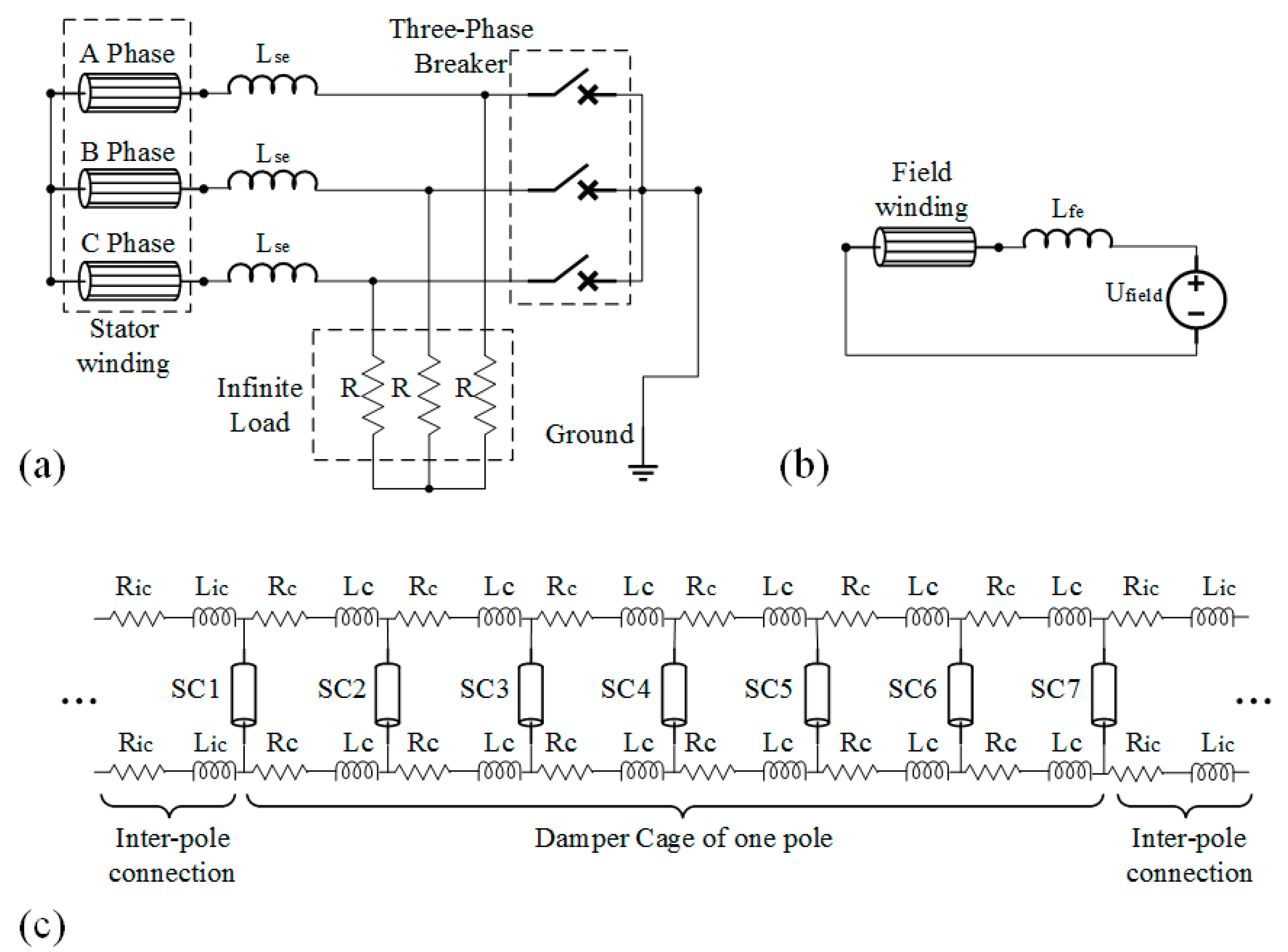
The external circuits are set and linked to the 2-D FE model as shown in Figure 4 to perform the simulation of the test, as shown in Figure 5. The resistances of the stator and field windings can be accurately calculated by using an analytical solution from design data and are set in the winding components in the external circuit. The end leakage inductance of the stator and field windings (L_se and L_fe in Figure 5), damper cage end ring equivalent resistance, and end leakage inductance of the adjacent bars (R_c, L_c, R_ic, L_ic) are also obtained analytically [12,14]. The external circuit parameters are summarized in

Table 2. External circuit parameters.

Name	Value
Stator winding phase resistance	0.238 Ω
Lse	4.3 mH
Rc	7 μΩ
Ric	27 μΩ
Infinite load R	10 MΩ
Field winding resistance	36 Ω
Lfe	153 mH
Lc	0.034 μH
Lic	0.12 μH

. In the three-phase sudden short-circuit test, the SPSM is driven by the prime mover, typically a motor in the Power System Dynamic Simulation Laboratory; hence, the fluctuation of the rotation speed can be neglected. The rotor rotation speed is therefore constant at the rated synchronous speed in the mechanical setting of the time-stepping FE model.

The 2-D static magnetic field FE model has the same geometry as the field-circuit coupled time-stepping FE model and is applied to calculate the inductances.

To consider the skin effects of the damper bars, each damper bar is divided into several segments in the 2-D FE model. The current information recorded in the field-circuit FE simulation is imported into the static magnetic FE simulation to produce a magnetic flux distribution similar to the flux distribution in time-stepping FE solution for accurately computing the inductances.

3.2. Calculation Procedure

The procedure to calculate the transient d-q axis reactance parameters is described as follow.

Step 1: The three-phase sudden short-circuit test is simulated using the 2-D field-circuit coupled time-stepping FE model. The total currents of the stator windings (I_A, I_B, I_C), field winding (I_F) and each segment of each damper bar (I_b11, I_b12, …, I_b18, I_b21, I_b22, …) are obtained and exported in the simulation results at each time step in the whole simulation time range. The rotor position at each time step is also recorded. All currents and rotor position data are related to the time instants.

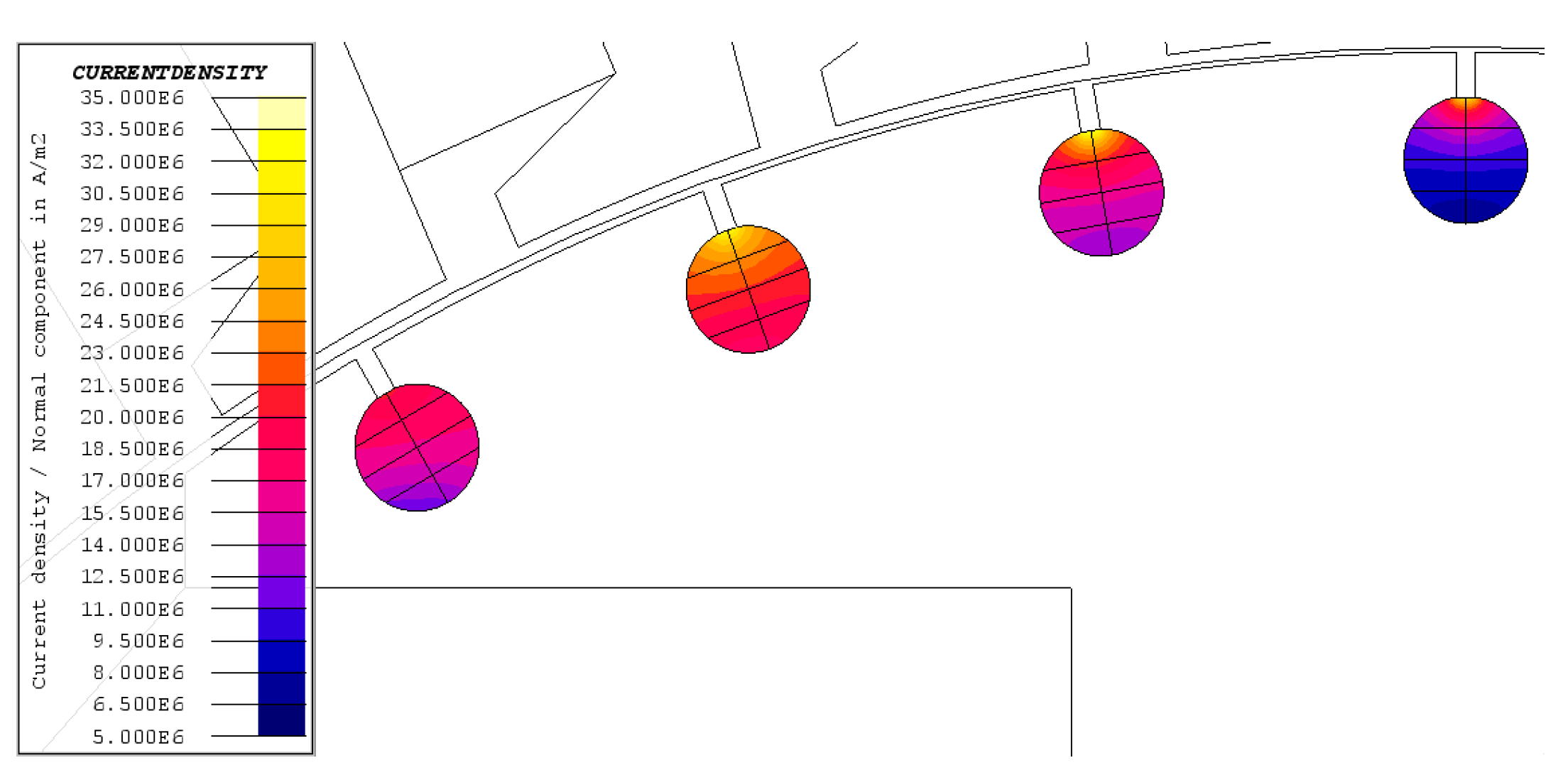
Each damper bar is divided into eight geometric segments in the 2-D FE model to consider the skin effects mentioned in Section 3.1 As the current density of each segment and the damper bar can be obtained from MVP calculated in the FE solution, the total current of each segment in each damper bar can be obtained by using Equation (8). The current density distributions of the damper bar segments are shown in Figure 6.

$$I_{bki}={\displaystyle {\iint }_{S_{ki}}(j\omega \sigma A_{bki})}dS+\frac{\sigma U_{bk}}{l_{ef}}{S}_{ki}\begin{array}{cc},& I_{bk}={\displaystyle \sum _{i=1}^8{I}_{bki}}\end{array}$$

(8)

where A_bki is the MVP in the damper bar region, U_bk is the voltage drop of the damper bar, σ is the conductivity of the conductor bar, l_ef is the effective length, k represents the serial number of the damper bar and i is the serial number of the segments in a bar region. I_bk represents the total current of a damper bar and I_bki is the current of a segment in a damper bar. S_ki is the integration region of each segment.

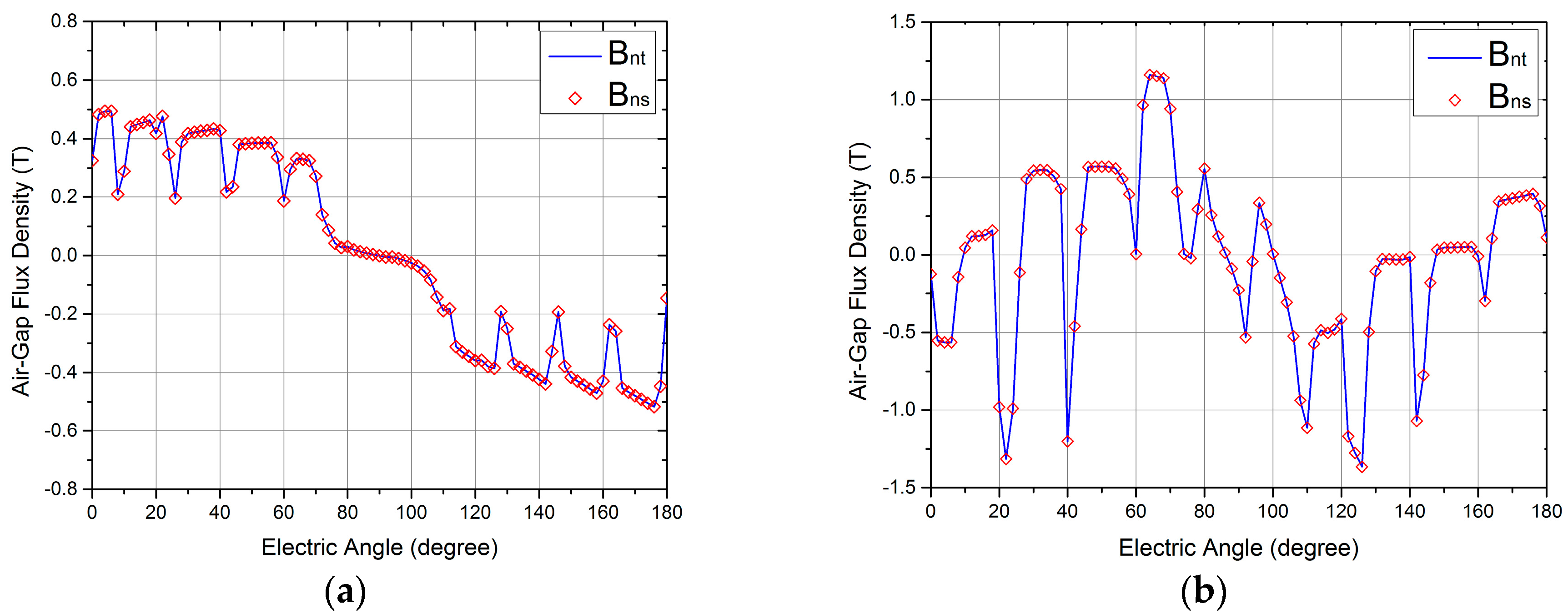
Step 2: The recorded currents and rotor positions at each calculation time instant are imported into the 2-D static magnetic FE model to obtain the same magnetic field distribution as the time-stepping transient FE application in step 1. As shown in Figure 7, the air-gap flux density distributions are the same for the field-circuit coupled time-stepping FE application in step 1 and the static magnetic FE simulation in step 2. Therefore, the magnetic field distribution and iron saturation condition in both simulations are nearly uniform. It is difficult to obtain the inductance directly; hence, the inductance computed by using the iron saturation condition in the static magnetic FE application, carried out in step 2, can accurately represent the flux distribution of the field-circuit FE application obtained in step 1. The frozen permeability method is applied to record the core saturation information of the results in step 2 for inductance computation in step 3. In this method, the permeability of all the mesh elements in the stator and rotor core regions of the results in step 2 is frozen and exported, corresponding to the time instants, as the permeability distribution can represent the iron saturation condition.

Step 3: After freezing the permeability, the kD or kQ model is implemented in the circuit set of damper bar components in the static FE circuit model, corresponding to the time instants. The mesh elements in the model must remain unchanged. By importing the frozen permeability of each mesh element obtained in step 2 into the same mesh elements in the same core region, the iron saturation condition in step 2 is reproduced in the FE model of step 3 by the same permeability distribution in core regions. 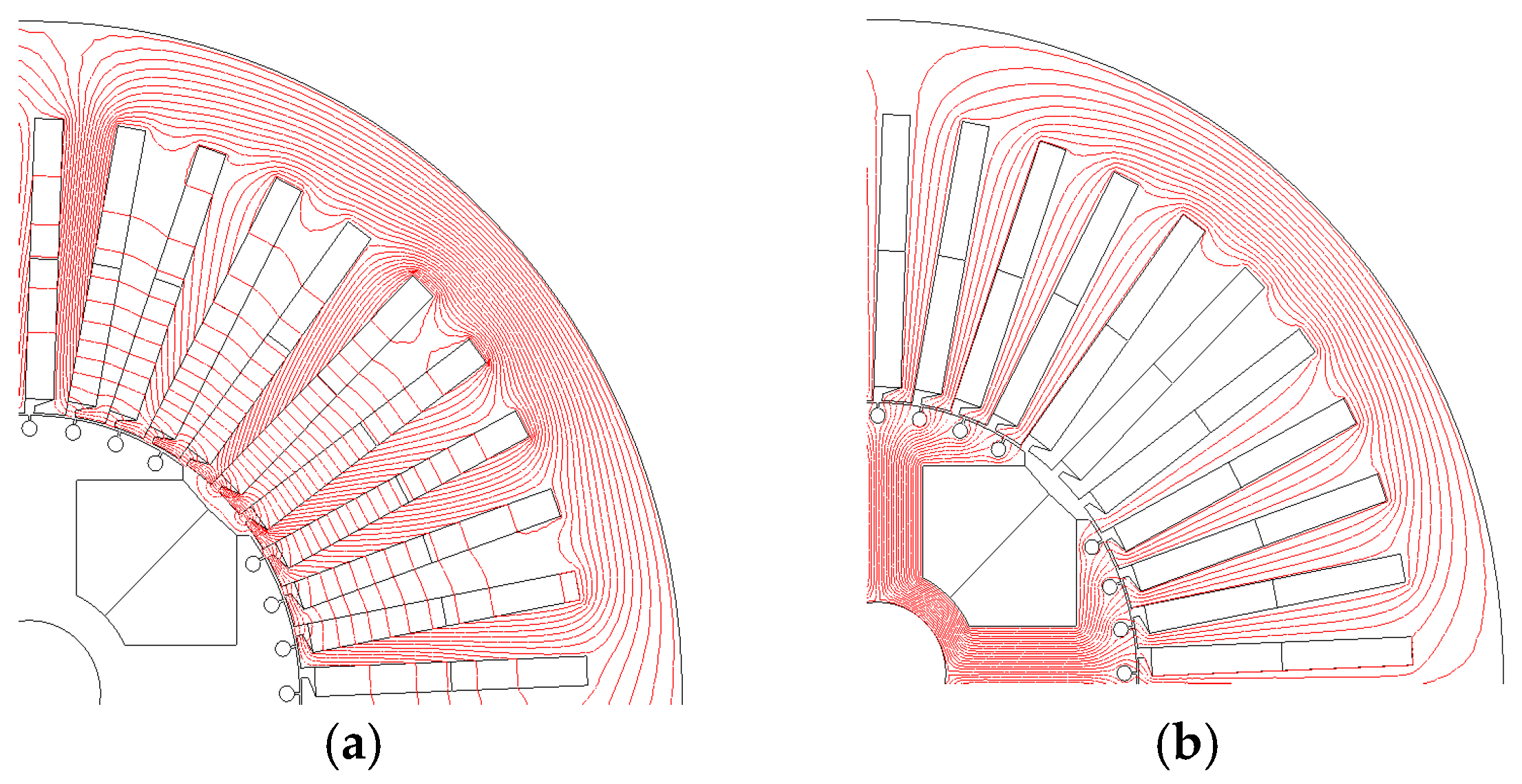The inductances are calculated with the method presented in Section 3.3

The flux distributions at the no-load condition before the short-circuit in Figure 7a and at the transient condition after the short-circuit in Figure 7b are vastly different. The variation in the flux distribution can lead to variation in the inductances of the SPSM, including leakage inductances; therefore, the variation should be investigated and considered in the computation. To calculate the inductance variation, a recursive inductance calculation is applied to each chosen time instant during the entire period, from the short-circuit to the steady short circuit state—referred to as the transient process in this paper. For simplification, only 2p (p represents pole pairs) of one rotation cycle is needed to calculate the d- and q-axis inductances to represent the inductance variation. Thus, in the period, the d-axis inductances are calculated at the time instants when the d-axis meets the stator A phase winding axis; the q-axis inductances are calculated similarly. Steps 2 and 3 are carried out and repeated at each chosen time instant of the transient process.

3.3. Inductance Calculation

In the stator self-leakage inductance calculation, the frozen permeability of the stator core is imported into the FE model [18]. The rotor parts in the FE model should be removed to extract the stator self-leakage magnetic field. Technically, a boundary between the rotor region and air gap region is built in to the FE model. The boundary condition is set the same as Equation (7). Thus, the excitation of stator currents can only generate stator self-leakage field in the model. The self-leakage inductance can be obtained using the stored magnetic energy computation and circuit equations as described in [14]. At the time instants when the d-axis meets the A phase winding axis, the d-axis stator self-leakage inductance is calculated, as shown in Equations (9)–(11). As the non-linear core regions are processed linearly by the frozen permeability method, the influence of non-linear core saturation is considered in inductance calculation. Besides, after the linear processing, both the field Equation (9) and circuit Equation (10) can be used in this case for stator self-leakage inductance computation.

$$W_m=l_{ef}{\displaystyle \underset{S}{\iint }({\displaystyle {\int }_0^{B}HdB)}ds}$$

(9)

$$W_m=0.5{\displaystyle \sum _{i,j=A,B,C}{L}_{ij}{I}_i{I}_j}=0.5{\displaystyle \sum _{i=A,B,C}{L_s}^{\prime }{I_i}^2}+{\displaystyle \sum _{\begin{array}{l}\begin{array}{cc}& \end{array}i\ne j\\ i,j=A,B,C\end{array}}{M_s}^{\prime }{I}_i{I}_j}$$

(10)

where W_m is the stored magnetic energy for the whole domain, S is the integration region, H is the magnetic field intensity and B is the magnetic flux density. L_s’ is the self-inductance of the stator phase winding, and M_s’ is the mutual inductance between two phase windings.

In step 3 of the static FE simulation, I_A is set to 1 A, and I_B and I_C are set to −0.5 A. W_m can be directly obtained from Equation (9) by using the FE result. As only the stator self-leakage magnetic field is generated, L_s’ and M_s’ are equal to the self-leakage inductance of a stator phase winding (L_spσ) and the mutual leakage inductance between two stator phase windings (M_spσ), respectively, in this simulation [14]. Thus, the currents in Equation (10) and result of Equation (9) are applied in Equation (11) to obtain the d-axis stator self-leakage inductance.

$$\begin{array}{l}{W}_m=0.75({L_s}^{\text{'}}-{M_s}^{\text{'}})=0.75(L_{sp\sigma }-M_{sp\sigma })=0.75L_{sld}\\ L_{sld}=\frac{4l_{ef}}{3}{\displaystyle \underset{S}{\iint }({\displaystyle {\int }_0^{B}HdB)}dS}\end{array}$$

(11)

where L_sld is the d-axis stator self-leakage inductance.

The flux distribution of the stator d-axis winding’s self-leakage flux is shown in Figure 8a. The same method is employed to compute the q-axis stator self-leakage inductance at the time instants when the q-axis meets the stator A phase winding axis. Additionally, the self-leakage inductances of the field and damper windings are calculated by importing the rotor frozen permeability magnetic characteristic setting in the FE model, exciting only I_F, I_D, or I_Q.

The flux linkages of windings are obtained from MVP computed by FE solutions, as shown in Equation (12). The d- and q- axis flux linkages are calculated when the d-axis and q-axis meet with the stator A phase winding axis, respectively.

$$\begin{array}{l}{\psi }_i=\frac{l_{ef}{\displaystyle \sum _{k=1}^{\beta }(A_{Uk}-A_{Lk})}}{I_F}\begin{array}{cc}& (i=A,B,C,f,kD,kQ)\end{array}\\ {\psi }_j=\frac{2}{3}({\psi }_A-\frac{1}{2}{\psi }_B-\frac{1}{2}{\psi }_C)\begin{array}{cc}& (j=d,q)\end{array}\end{array}$$

(12)

where A_Uk and A_Lk are the MVP of the upper and lower sides of coil k in winding i, respectively, β is the total number of coils in winding i, l_ef is the axial effective length of prototype.

The frozen permeabilities of the stator and rotor cores are imported into the FE model to calculate the armature reaction inductances. Only I_F is excited to calculate the mutual inductance between the stator d-axis winding and field winding M_adf, and only I_Q is excited to calculate the mutual inductance between the stator q-axis winding and kQ winding M_aqQ. The armature reaction inductances are calculated as:

$$\begin{array}{l}{M}_{adf}=\frac{{\psi }_d}{I_F}\begin{array}{cc},& L_{ad}=\frac{M_{adf}}{i_b}{i}_{fb}\end{array}\\ M_{aqQ}=\frac{{\psi }_q}{I_Q}\begin{array}{cc},& L_{aq}=\frac{M_{aqQ}}{i_b}\end{array}{i}_{Qb}\end{array}$$

(13)

where ψ_d and ψ_q are the flux linkages of the d- and q-axis stator windings, respectively, i_b, i_fb, and i_Qb are the P.U. current base values of the stator winding, field winding, and kQ damper winding, respectively. The flux distribution of only I_F excitation to compute M_adf is shown in Figure 8b.

The gap leakage inductances are also calculated by importing both the stator and rotor permeabilities. The stator gap leakage inductance of the d-axis is calculated in Equation (14). The q-axis gap leakage inductances are obtained in a similar manner. The field gap leakage inductance is computed in Equation (15), and the gap leakage inductances of kD and kQ windings are obtained similarly.

$$L_d=\frac{{\psi }_d}{I_d}\begin{array}{cc},& \end{array}{L}_{slgd}=L_d-L_{ad}-L_{sld}$$

(14)

$$L_{ff}=\frac{{\psi }_f}{I_F}\begin{array}{cc},& \end{array}{L}_{flg}=L_{ff}-L_{fl}-L_{ffd}\begin{array}{cc},& \end{array}{L}_{ffd}=\frac{2}{3}{L}_{ad}{(\frac{i_b}{i_{fb}})}^2$$

(15)

The length of the transient process from the short-circuit to the steady short state is measured by a transient FE application. The transient process consists of a subtransient process as the period of the damper current attenuation, until the aperiodic component of the damper current decays to less than 5 percent of the initial value. The leakage inductance of the damper windings is computed for all the chosen time instants in the subtransient process; the other leakage inductances are obtained for all the chosen time instants during the whole transient process.

Finally, the subtransient and transient reactances x_d″, x_q″, and x_d’ for each selected time instant are calculated on a P.U. basis in Equations (4) and (5) by separately transferring all inductances to a P.U. basis.

The subtransient reactance parameters X_d″ and X_q″, as well as the transient reactance parameter X_d’, of the SPSM are defined as the mean value of x_d″, x_q″, and x_d’ at all time instants from the short-circuit to the time when the transient aperiodic component of the kD, kQ, and field winding currents, respectively, decay to 20% of the initial value; here, the saturation variation in the constant terminal reactance parameters of the SPSM is taken into account.

3.4. Time Constant Computation and Developed Program

The short-circuit time constants T_d″, T_q″, T_d’, and T_a are obtained by curve fitting and applying the Prony algorithm. The Prony algorithm exponentially provides the frequency, magnitude, and damping factor information for all modes of the imported discrete transient signal. As described in [19], the Prony algorithm and least squares algorithm are used to determine the short-circuit time constant. The mathematical model of the Prony algorithm is shown in Equations (16) and (17).

$$\widehat{y}(k)={\displaystyle \sum _{i=1}^n{B}_i{Z_i}^k}\hspace{0.17em}\hspace{0.17em}\hspace{0.17em}\hspace{0.17em}(k=0,1,···,N-1)$$

(16)

$$B_i=A_i\exp (\mathrm{j}{\theta }_k),\hspace{0.17em}\hspace{0.17em}\hspace{0.17em}{Z}_i=\exp ({\alpha }_i\Delta t)\cdot \exp (\mathrm{j}2\pi f_i\Delta t)$$

(17)

where $\widehat{y}(k)$ is the approximate representation of sampling current signal. n is the number of total harmonics of the signal, and A_i, θ_i, B_i, α_i, and f_i are the peak value, phase, amplitude, damping factor, and frequency of each exponential harmonic component of the fitting current, respectively. The time constant of the harmonic component, obtained by the damping factor, is:

$$T_i=-\frac{1}{{\alpha }_i}$$

(18)

In the presented method, the d-axis short-circuit time constant, including the d-axis subtransient short-circuit time constant T_d″ and the d-axis transient short-circuit time constant T_d’, is estimated from the armature short-circuit current using the Prony algorithm; the armature short-circuit time constant T_a is also estimated this way. The q-axis subtransient short-circuit time constant T_q″ is obtained from the kQ current waveform.

3.5. Developed Program

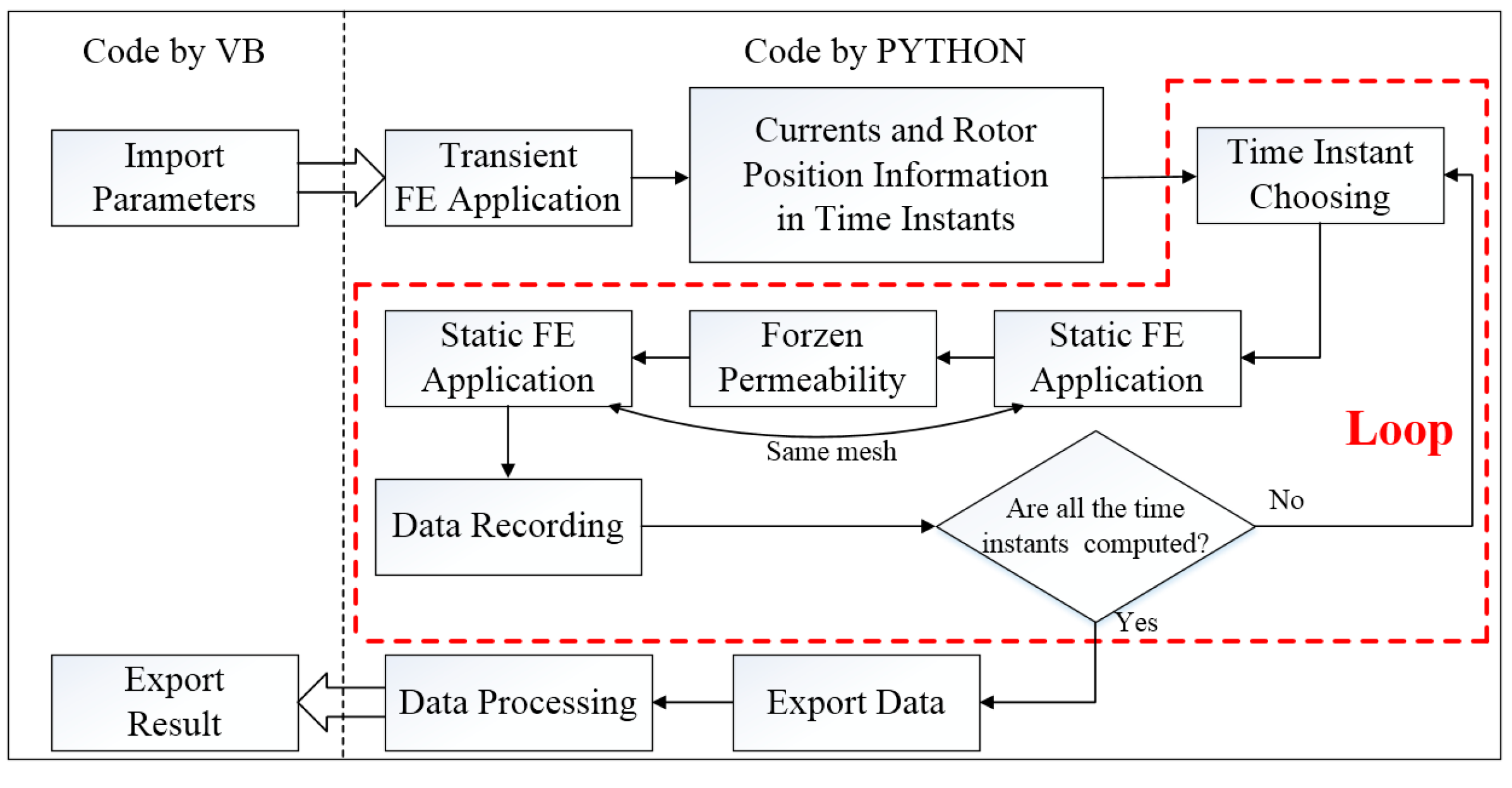
To address the complex simulation and data processing, a program is developed by employing PYTHON and visual basic to control the commercial FE software and data processing. The entire calculation is automatic after applying the program to the FE model. The structure of the program is shown in Figure 9. In this program, a loop process of inductances computation whose calculation methods are described in Section 3.3 is applied to compute the inductances in each chosen time instants.

4. Results and Comparison

The transient parameters of the prototype are determined based on the abovementioned model and methods. All inductances are transferred to reactances in X_ad P.U. basis, and the time instant of three-phase sudden short circuit is set to 0 s in this section.

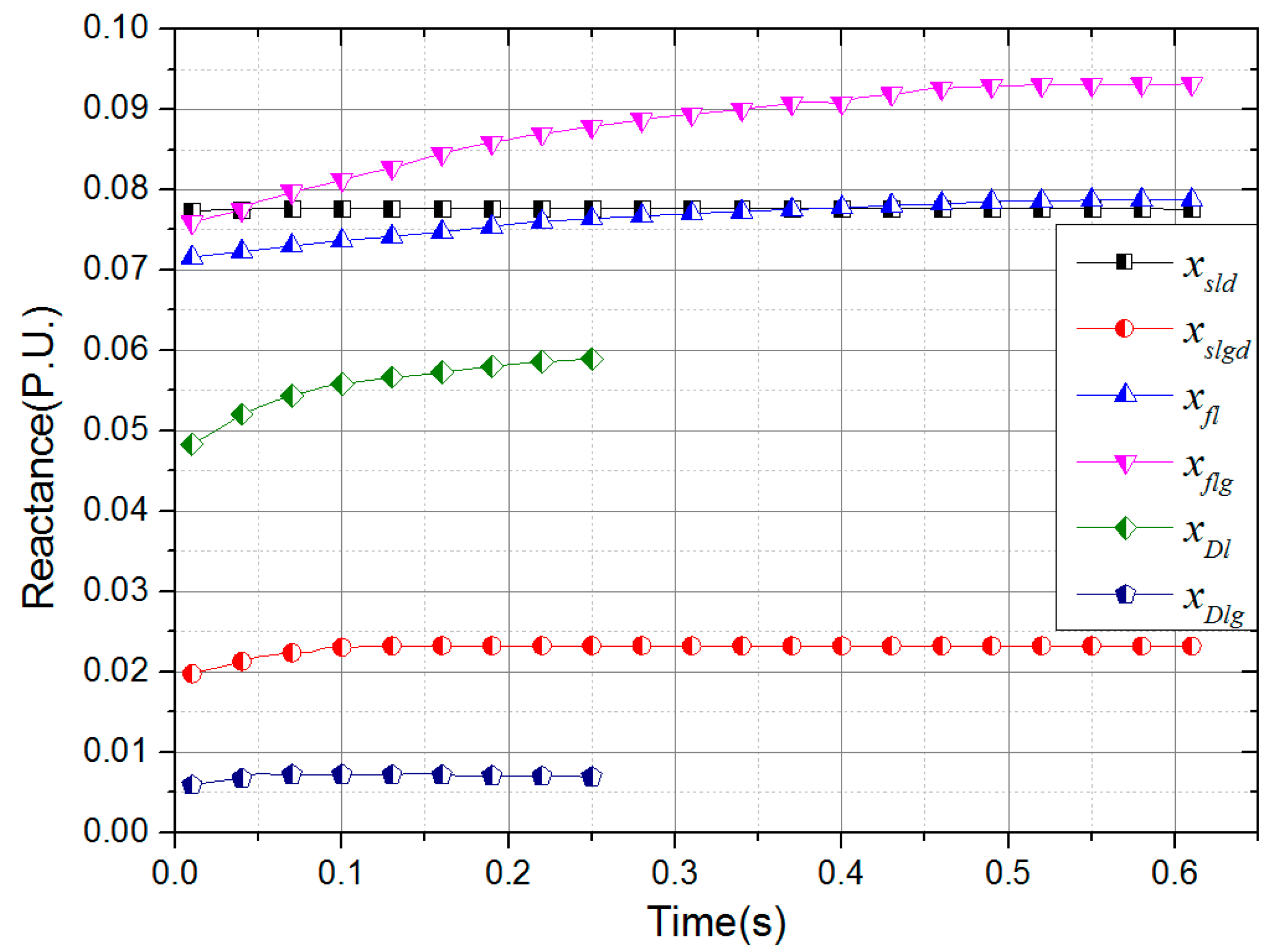
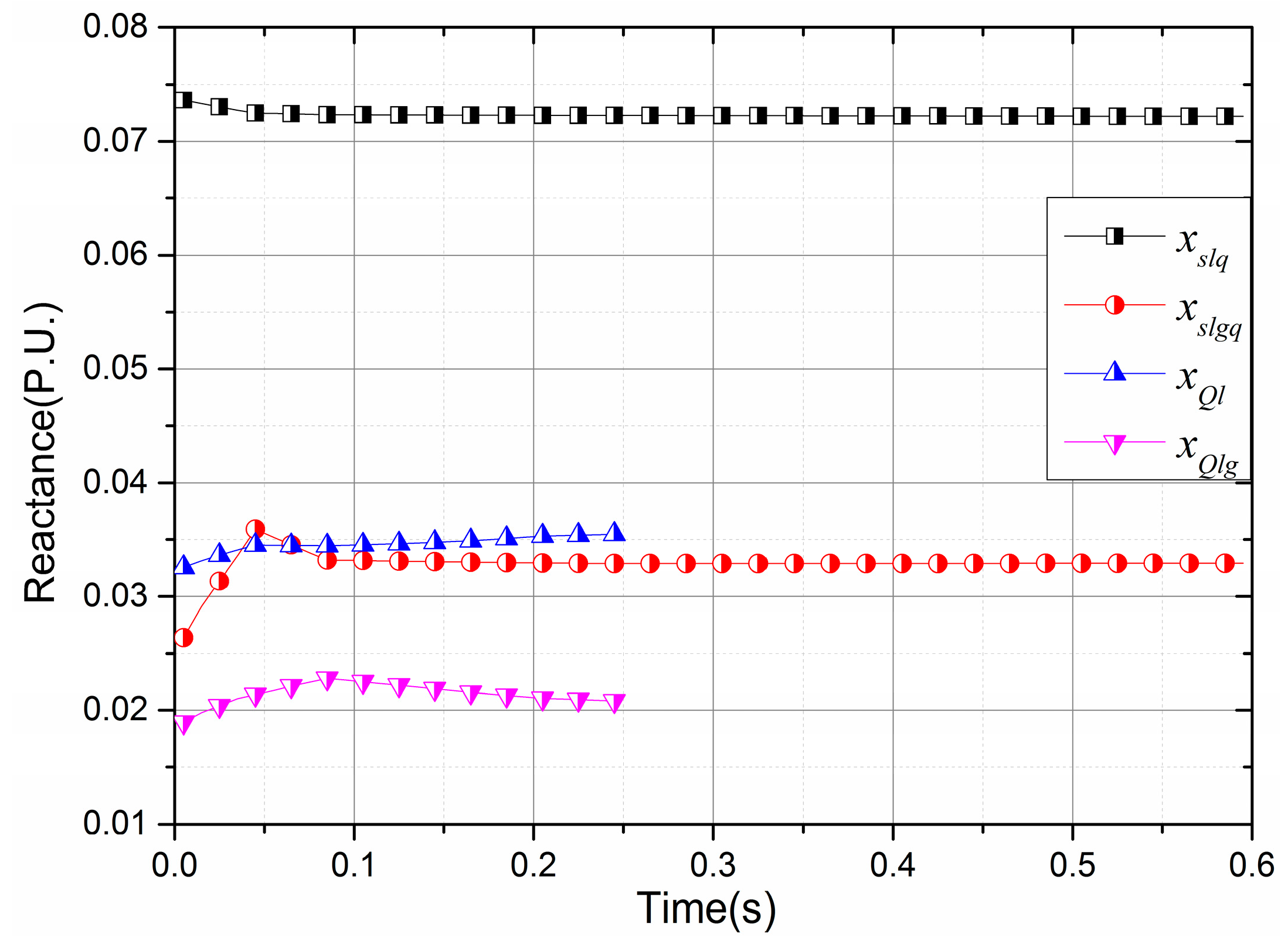
The leakage inductances of stator, field, and damper windings and their variations in the d- and q-axes are shown in Figure 10 and Figure 11, respectively. It is shown that the gap leakage inductances play a significant role in the leakage inductances, particularly for the field winding. If the gap leakage inductances are neglected, as in the traditional design and analysis of an SPSM, the leakage inductances may be inaccurately estimated.

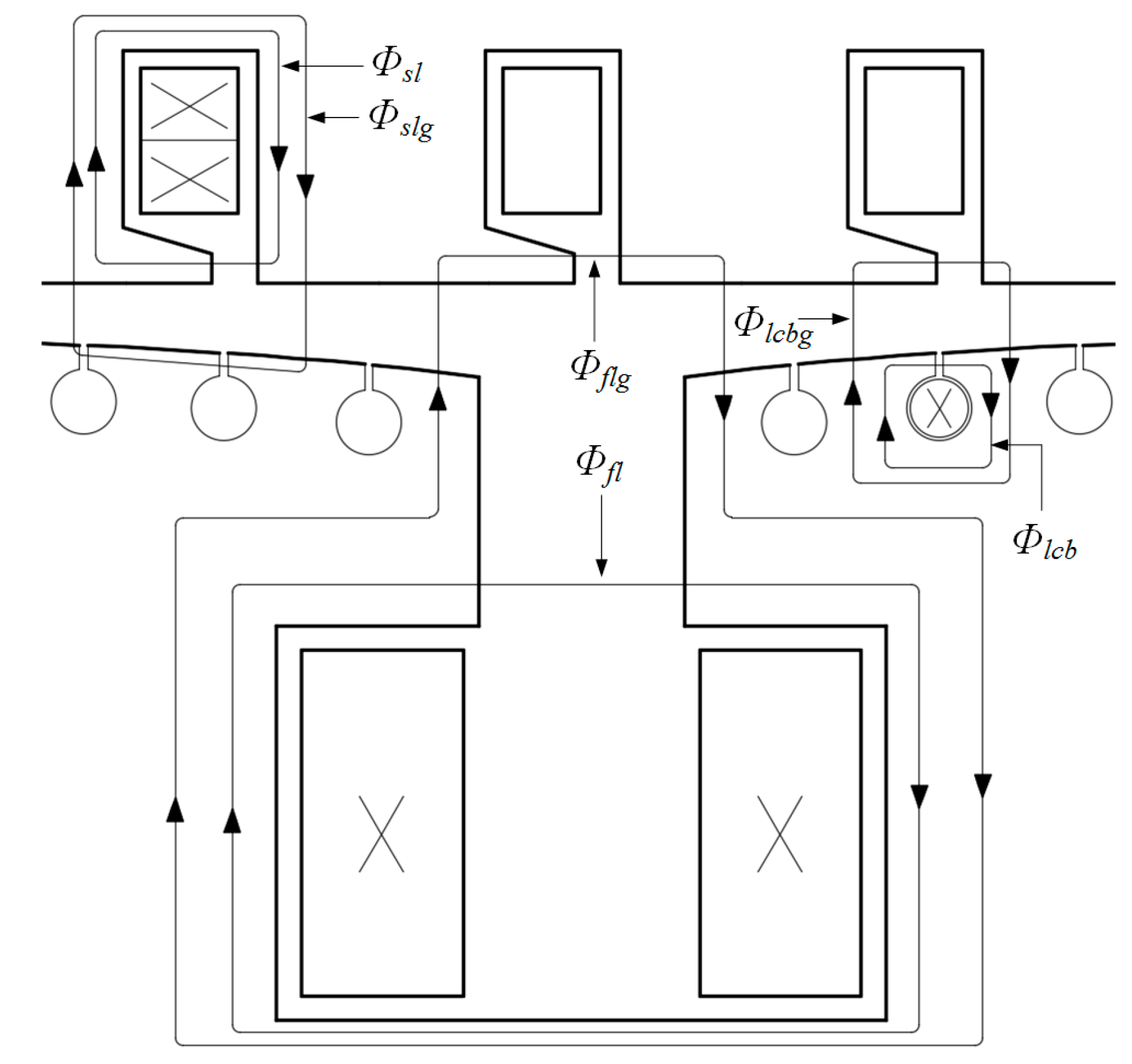
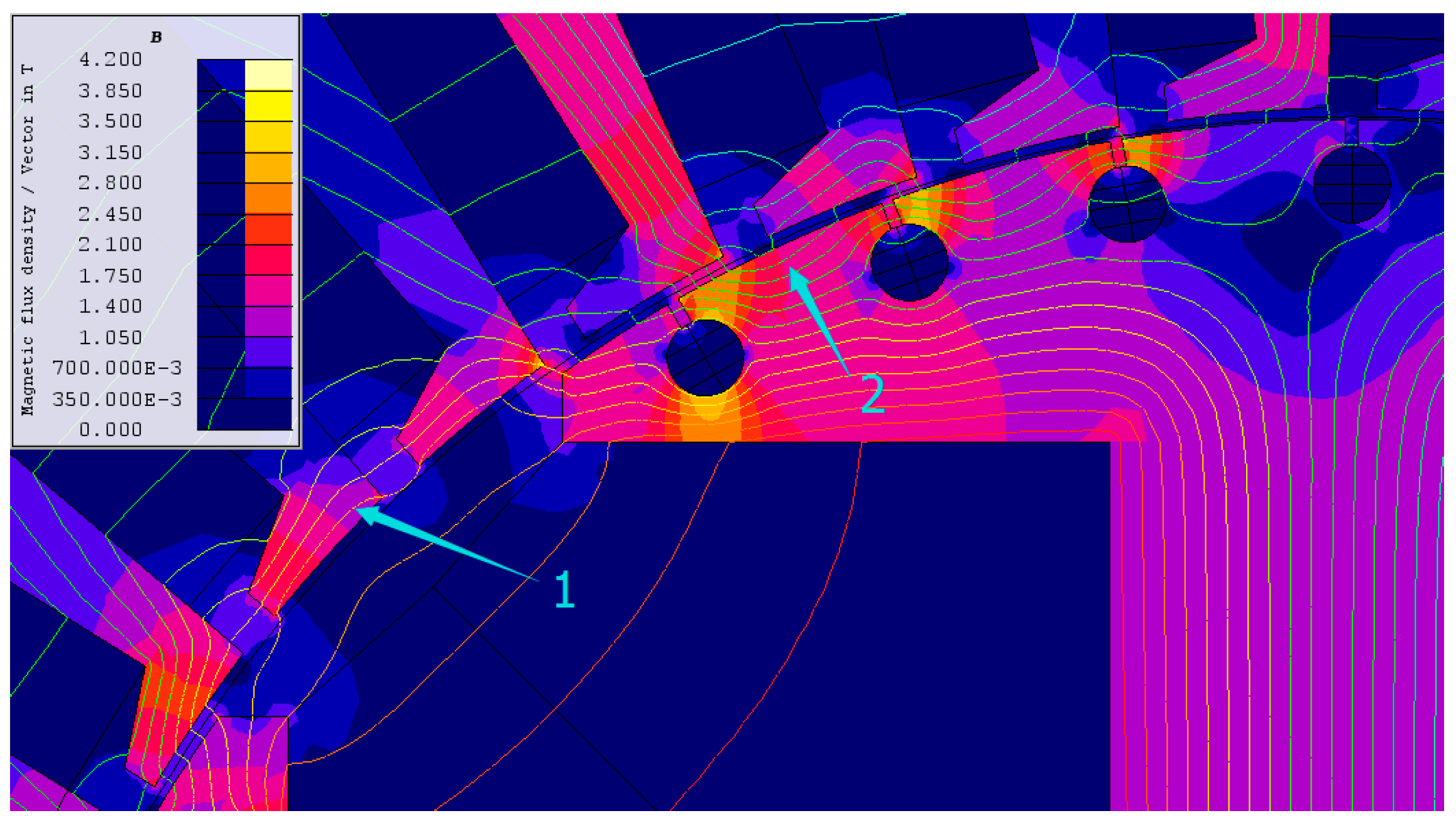
The magnetic flux line of the gap leakage flux, shown in Figure 12, verifies the leakage inductance model. Arrow 1 illustrates the field winding gap leakage flux line flowing through the pole shoe, air gap, and stator slot opening; Arrow 2 indicates the stator winding gap leakage flux line mainly flowing across the air gap and damper cage tooth. Compared to the megawatt-class SPSM, such as a large hydro-generator [13,14,15], the gap leakage inductance is more evident in a kilowatt-class SPSM due to the differences in geometric design, including a semi-closed stator slot and a short air gap length.

Figure 10 and Figure 11 also show that the leakage inductances are not constant in the transient process, particularly for the damper and field windings. The fluctuation is caused by variation of core saturation during the transient process. However, the variations in the self-leakage inductance of the stator windings are small, which indicates that the saturation variation mainly occurs in the pole shoe and pole tip, specifically between the damper cage slot and shoe edge, as shown in Figure 12. The flow through the damper cage is avoided by induced currents for conservation of flux linkage; therefore, the main flux flows through the path between the damper slot and shoe edge, leading to saturation in that area. As seen in Figure 12, there is increased saturation in the preliminary stage of the transient process after the short-circuit. In addition, the transient currents decay to the steady short-circuit state and thereby alleviate the saturation, as illustrated in the growing leakage inductances in Figure 10 and Figure 11. Therefore, the traditional theory that ignores the saturation variation in the leakage inductance computation and dynamic analysis is not impeccable. The variation of the leakage inductances should be considered to acquire precise dynamic performance. In an effort to eliminate the influence of saturation in transient processes, designers should optimize the geometry of the pole shoe and damper cage slot in the design stage.

It is difficult to precisely consider the skin effects, the saturation, and magnetic distortion in the analytical solution when attempting to estimate generator performance. It is also difficult to determine the detailed characteristics of the machine from terminal data. Thus, the FE analysis should be applied for SPSM design.

The transient aperiodic component of the kD, kQ, and field winding currents can be easily obtained by the time-stepping FE simulation and data processing. The time lengths of the transient current aperiodic component attenuation from the short circuit to 20% of the initial value of the kD, kQ, and field windings, considering the calculation time instants of each winding, are approximately 0.08 s, 0.125 s, and 0.24 s, respectively. The subtransient and transient reactances x_d″, x_q″, and x_d’ at each calculation time instant are shown in

Table 3. Subtransient and transient reactance parameters values at calculation time instants.

Time (s)	xd’’ (P.U.)	xd’ (P.U.)	Time (s)	xq’’ (P.U.)
0.01	0.1650	0.2713	0.005	0.1651
0.02	0.1667	0.2731	0.015	0.1688
0.03	0.1682	0.2749	0.025	0.1726
0.04	0.1698	0.2766	0.035	0.1752
0.05	0.1713	0.2788	0.045	0.1785
0.06	0.1719	0.2799	0.055	0.1813
0.07	0.1727	0.2810	0.065	0.1810
0.08	0.1730	0.2816	0.075	0.1806
0.09	-	0.2830	0.085	0.1802
0.10	-	0.2837	0.095	0.1798
0.11	-	0.2844	0.105	0.1797
0.12	-	0.2851	0.115	0.1796
0.13	-	0.2857	0.125	0.1795
0.14	-	0.2864	-	-
0.15	-	0.2871	-	-
0.16	-	0.2878	-	-
0.17	-	0.2884	-	-
0.18	-	0.2890	-	-
0.19	-	0.2895	-	-
0.20	-	0.2900	-	-
0.21	-	0.2906	-	-
0.22	-	0.2909	-	-
0.23	-	0.2912	-	-
0.24	-	0.2916	-	-
Mean Value (P.U.)	0.1698	0.2842	-	0.1770

.

The mean values of the subtransient and transient reactances in each computation time instants, shown in Table 3, are the subtransient and transient reactance parameters of the prototype computed by the presented method. A comparison of the prototype experimental values and the transient parameters calculated using both the proposed and conventional short-circuit methods [3] is shown in

Table 4. External Circuit Parameters.

Parameter	Short-Circuit Method Value (P.U.)	Novel Method Value (P.U.)	Experimental Value (P.U.)	Error between Novel Method and Experiment
Xd’’	0.178	0.1698	0.172	1.2%
Xd’	0.332	0.2842	0.290	2%
Xd	1.786	1.7392	1.705	2%
Xq’’	-	0.1770	0.170	4.2%
Xq	-	1.1738	1.130	3.9%

.

The experimental value of the prototype is provided by the Power System Dynamic Simulation Laboratory where the presented prototype is installed and applied for dynamic simulation experiments. The experimental methods recommended in standard [11] are applied to obtain the experimental transient parameters of the prototype, including transient and steady state reactances.

The comparison demonstrates the accuracy of the proposed method for computing the transient reactance parameters.

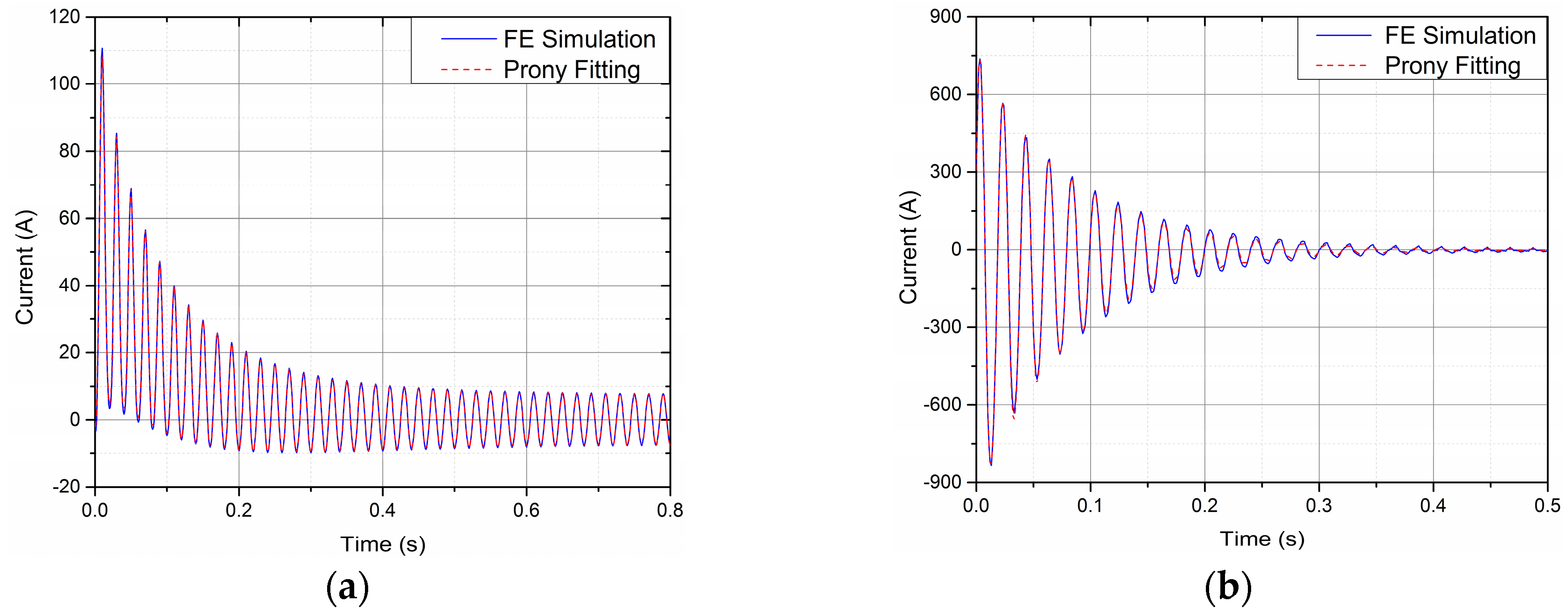
The waveforms of the stator A phase winding current and kQ winding current, obtained by the time-stepping FE simulation, are imported into a Prony algorithm-based data processing program to compute the time constant parameters, as described in Section 3.4. The comparison of the FE simulated current and Prony algorithm fitting current are illustrated in Figure 13, and the main modal information of the fitting current is shown in

Table 5. Modal identification of fitted current.

Modal Information	Mode	Amplitude	Damping Factor	Frequency
Modal information of stator A phase short-circuit current	1	110	−12	0
	2	28	−6.7	50
	3	28	−6.7	−50
	4	19	−24	50
	5	19	−24	−50
	7	7.1	0.0	50
	8	7.1	0.0	−50
	9	8.9	−12	100
	10	8.9	−12	−100
Modal information of kQ short-circuit current	1	110	−13	0
	2	820	−12	50
	3	820	−12	−50

.

There is little error between the simulated current and fitted current waveforms, as illustrated in Figure 13. Hence, the modal information obtained from the fitting current waveform can be applied to precisely estimate time constants of each component’s current obtained from the FE simulation. The components of a short-circuit current have been previously described [12]. In the modal information of the stator short-circuit current, mode 1 is the aperiodic component of the short-circuit current, and mode 2/3 and mode 4/5 represent the d-axis transient and subtransient AC components, respectively. Mode 7/8 and mode 9/10 denote the d-axis steady state AC component and second harmonic frequency AC component, respectively. In the modal information of the kQ short-circuit current, mode 1 is the DC component, while mode 2/3 represents the rotating frequency AC component. Each time constant can be obtained from the damping factor of the corresponding mode. The time constants and their comparison with the conventional method [11] and experimental results are shown in

Table 6. Comparison of transient time constant parameters.

Parameter	Short-Circuit Method Value (s)	Novel Method Value (s)	Experimental Value (s)
Td’’	0.065	0.042	0.036
Td’	0.220	0.149	0.160
Tq’’	-	0.077	0.065 (design value)
Ta	0.095	0.083	0.078

. In Table 6, T_d’’, and T_d’ are the d-axis subtransient and transient short-circuit time constant respectively, T_q’’ is the q-axis subtransient short-circuit time constant and T_a is the armature short-circuit time constant. The comparison validates that the new method for computing the time constants of transient parameters is effective and accurate.

In the simulation and computation of this work, a personal computer (PC) with Intel^® Xeon CPU E3-1230 V2 @ 3.3 GHz and 16 GB random-access memory (RAM) is used. And the whole computation time interval applying the developed program is about 5 h and 30 min. All the presented results can be automatically calculated by the developed program.

Generally, as the aforementioned results and discussions shown, the results reveal that the gap leakage inductances and inductance variation during transient processes have significant influences on transient parameters and should be considered in computation to obtain more precise transient parameters. As shown in Figure 10 and Figure 11, the proposed method could extract the detailed leakage inductances separately in each computation time instant. Thus, a clear understanding of leakage inductances saturation and variation during a transient process could be obtained. Some phenomena of core saturation in transient process are investigated. Detailed information of leakage inductances can be provided to designers by this method for geometric optimization. The accuracy of the proposed method in transient parameters computation is validated by the comparison with experimental and conventional method results. The proposed method has turned out to be an effective method for the transient parameter computation and transient performance optimization of an SPSM.

5. Conclusions

This paper presents a novel method for calculating the transient parameters of an SPSM with a damper cage. A modified model is proposed to accurately calculate the leakage inductances, and FE analysis is used to consider the skin effects and saturation. By using this method, the leakage inductances of the magnetic equivalent circuit are separately obtained, and the inductance variation during the transient process is also investigated and discussed. The Prony method is applied to simulate the current waveform to estimate the time constant parameters. The complex FE analysis and data processing can be automatically performed by the developed program.

In the proposed method, the gap leakage inductances and inductances variation during transient process are considered, which makes the computation results precise. The detailed inductances in each time instant during a transient process can be extracted separately, which could help designers for optimization and refinement. Besides, as the transient inductances are calculated from detailed inductances and time constants are computed by curve fitting of the current waveform, parameter determination becomes objective and automatic.

The accuracy of the present method is validated by comparing the results with the conventional method.