
Transmission Power and Antenna Allocation for Energy-Efficient RF Energy Harvesting Networks with Massive MIMO

Abstract
:1. Introduction
2. System Model and Problem Formulation
2.1. Notation
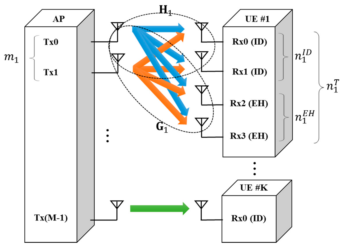
2.2. MU Massive MIMO RF-EHNs
2.3. Multi-User MIMO Channel Model
2.4. Channel Capacity of Multi-Antenna
2.5. Total Power Dissipation with Energy Harvesting
2.6. Overall Network Energy Efficiency
3. EE Optimization
3.1. Outer Loop Algorithm: Transformation of the Primal Objective Function
| Algorithm 1. Outer Loop Algorithm for EE Maximization. | |
| 1: | Set initial input , iteration index , threshold 𝜏 |
| 2: | While 1 do |
| 3: | Obtain optimum values of three arguments through the inner loop algorithm for the given |
| 4: | If (convergence verification) |
| 5: | Return and obtain optimal EE |
| 6: | else |
| 7: | Update and |
| 8: | end if |
| 9: | end while |
3.2. Closed-Form Expression for Outage Constraints
3.3. Inner Loop Algorithm: Resource Allocation
| Algorithm 2. Inner Loop Algorithm for Resource Allocation. | |
| 1: | Initialize: Active UE set |
| 2: | while are not converged do |
| 3: | for do |
| 4: | if do |
| 5: | Update by jointly solving (39)~(42) |
| 6: | Update by jointly solving (39)~(42) using the calculated value |
| 7: | Update by jointly solving (39)~(42) using the calculated value and |
| 8: | else if do |
| 9: | Update by jointly solving (39)~(42) |
| 10: | Update by jointly solving (39)~(42) using the calculated value |
| 11: | Update by jointly solving (39)~(42) using the calculated value and |
| 12: | end if |
| 13: | Update the subgradient of with |
| 14: | Update the subgradient of with |
| 15: | end for |
| 16: | Update the subgradient of with |
| 17: | Update the subgradient of with |
| 18: | Update the subgradient of with |
| 19: | Let |
| end while | |
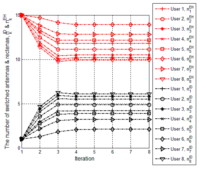
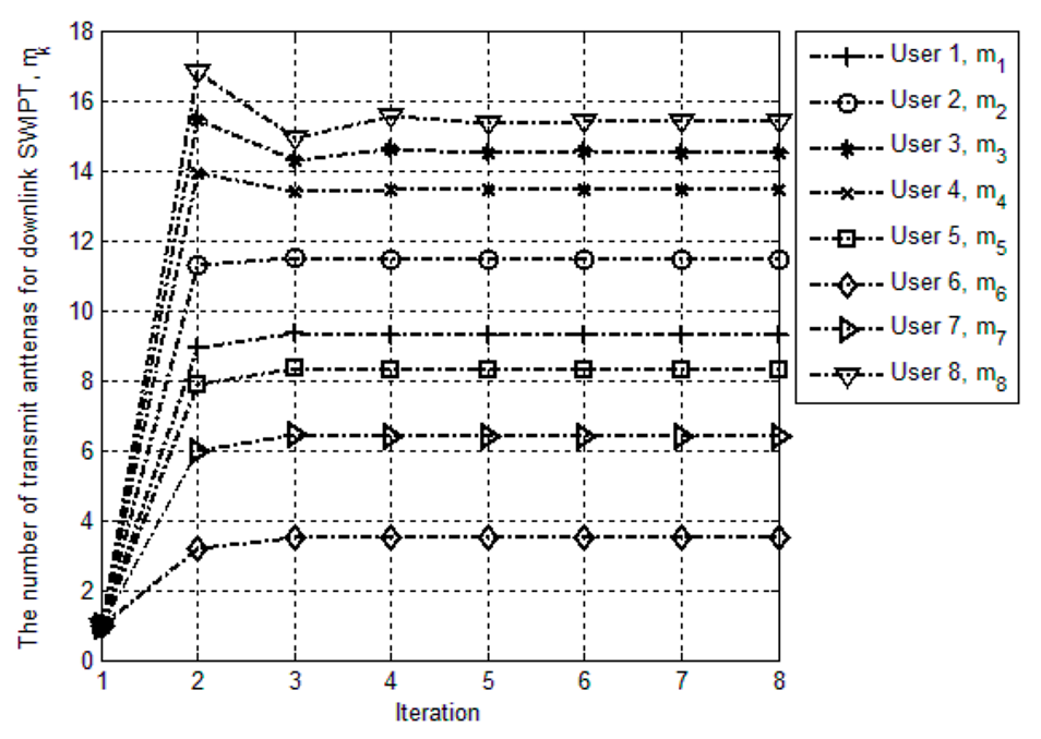
4. Simulation Results
5. Conclusions
Acknowledgments
Author Contributions
Conflicts of Interest
References
- Xiao, L.; Wang, P.; Niyato, D.; Kim, D.I.; Han, Z. Wireless networks with RF energy harvesting: A contemporary survey. IEEE Commun. Surv. Tutor. 2015, 17, 757–789. [Google Scholar] [CrossRef]
- Visser, H.J.; Vullers, R.J.M. RF energy harvesting and transport for wireless sensor network applications: Principles and requirements. Proc. IEEE 2013, 101, 1410–1423. [Google Scholar] [CrossRef]
- Lu, X.; Niyato, D.; Wang, P.; Kim, D.I.; Han, Z. Wireless charger networking for mobile devices: Fundamentals, standards, and applications. IEEE Trans. Wirel. Commun. 2015, 22, 126–135. [Google Scholar] [CrossRef]
- Zhang, R.; Ho, C.K. MIMO broadcasting for simultaneous wireless information and power transfer. IEEE Trans. Wirel. Commun. 2013, 12, 1989–2001. [Google Scholar] [CrossRef]
- Gesbert, D.; Shafi, M.; Shiu, D.; Smith, P. From theory to practice: An overview of space-time coded MIMO wireless systems. IEEE J. Sel. Areas Commun. (JSAC) 2003, 21, 281–302. [Google Scholar] [CrossRef]
- Yongxu, Z.; Kai-Kit, W.; Yangyang, Z.; Christos, M. Geometric power control for time-switching energy-harvesting two-user interference channel. IEEE Trans. Veh. Technol. 2016, 65, 9759–9772. [Google Scholar]
- Yang, G.; Ho, C.K.; Guan, Y.L. Dynamic resource allocation for multiple-antenna wireless power transfer. IEEE Trans. Signal Process. 2014, 62, 3565–3577. [Google Scholar] [CrossRef]
- Zhou, X.; Zhang, R.; Ho, C.K. Wireless information and power transfer in multiuser OFDM systems. IEEE Trans. Wirel. Commun. 2014, 13, 2282–2294. [Google Scholar] [CrossRef]
- Zhao, F.; Wei, L.; Chen, H. Optimal time allocation for wireless and power transfer in wireless powered communication systems. IEEE Trans. Wirel. Commun. 2016, 65, 1830–1835. [Google Scholar] [CrossRef]
- Mekikis, P.V.; Antonopoulos, A.; Kartsakli, E.; Lalos, A.S.; Alonso, L.; Verikoukis, C. Information exchange in randomly deployed dense WSNs with wireless energy harvesting capabilities. IEEE Trans. Wirel. Commun. 2016, 15, 3008–3018. [Google Scholar] [CrossRef]
- Mekikis, P.V.; Lalos, A.S.; Antonopoulos, A.; Alonso, L.; Verikoukis, C. Wireless energy harvesting in two-way network coded cooperative communications: A stochastic approach for large scale networks. IEEE Commun. Lett. 2014, 18, 1011–1014. [Google Scholar] [CrossRef]
- Kong, H.B.; Flint, I.; Wang, P.; Niyato, D.; Privault, N. Exact performance analysis of ambient RF energy harvesting wireless sensor networks with Ginibre Point Process. IEEE J. Sel. Areas Commun. 2016, 34, 3769–3784. [Google Scholar] [CrossRef]
- Zhou, X.; Zhang, R.; Ho, C.K. Wireless information and power transfer: Architecture design and rate–energy tradeoff. IEEE Trans. Wirel. Commun. 2013, 61, 4754–4767. [Google Scholar] [CrossRef]
- Ju, H.; Zhang, R. A novel mode switching scheme utilizing random beamforming for opportunistic energy harvesting. IEEE Trans. Wirel. Commun. 2014, 13, 2150–2162. [Google Scholar] [CrossRef]
- Moritz, G.L.; Rebelatto, J.L.; Souza, R.D.; Uchôa-Filho, B.F.; Li, Y. Time-switching uplink network-coded cooperative communication with downlink energy transfer. IEEE Trans. Signal Process. 2014, 62, 5009–5019. [Google Scholar] [CrossRef]
- Liu, L.; Zhang, R.; Chua, K. Wireless information and power transfer: A dynamic power splitting approach. IEEE Trans. Commun. 2013, 61, 3990–4001. [Google Scholar] [CrossRef]
- Timotheou, S.; Krikidis, I.; Zheng, G.; Ottersten, B. Beamforming for MISO interference channels with QoS and RF energy transfer. IEEE Trans. Wirel. Commun. 2014, 13, 2646–2658. [Google Scholar]
- Shi, Q.; Liu, L.; Xu, W.; Zhang, R. Joint transmit beamforming and receive power splitting for MISO SWIPT systems. IEEE Trans. Wirel. Commun. 2014, 13, 3269–3280. [Google Scholar] [CrossRef]
- Krikidis, I. Simultaneous information and energy transfer in large-scale networks with/without relaying. IEEE Trans. Commun. 2014, 62, 900–912. [Google Scholar] [CrossRef]
- Wu, Y.; Chen, X.; Yuen, C.; Zhong, C. Robust resource allocation for secrecy wireless powered communication networks. IEEE Commun. Lett. 2016, 20, 2430–2433. [Google Scholar] [CrossRef]
- Zhang, J.; Yuen, C.; Wen, C.-K.; Jin, S.; Wong, K.-K.; Zhu, H. Large system secrecy rate analysis for SWIPT MIMO wiretap channels. IEEE Trans. Inf. Forensics Secur. 2016, 11, 74–85. [Google Scholar] [CrossRef]
- Chen, X.; Yuen, C.; Zhang, Z. Wireless energy and information transfer tradeoff for limited feedback multi-antenna systems with energy beamforming. IEEE Trans. Veh. Technol. 2014, 63, 407–412. [Google Scholar] [CrossRef]
- Chen, X.; Wang, X.; Chen, X. Energy-efficient optimization for wireless information and power transfer in large-scale MIMO systems employing energy beamforming. IEEE Wirel. Commun. Lett. 2013, 2, 667–670. [Google Scholar] [CrossRef]
- Ju, H.; Zhang, R. Throughput maximization in wireless powered communication networks. IEEE Trans. Wirel. Commun. 2013, 13, 413–428. [Google Scholar] [CrossRef]
- Ju, H.; Zhang, R. Optimal resource allocation in full-duplex wireless powered communication network. IEEE Trans. Commun. 2014, 62, 3528–3540. [Google Scholar] [CrossRef]
- Amarasuriya, G.; Larsson, E.G.; Poor, H.V. Wireless information and power transfer in multiway massive MIMO relay networks. IEEE Trans. Wirel. Commun. 2016, 15, 3837–3855. [Google Scholar] [CrossRef]
- Al-Hraishawi, H.; Aruma Baduge, G.A. Wireless energy harvesting in cognitive massive MIMO systems with underlay spectrum sharing. IEEE Wirel. Commun. Lett. 2017, 6, 134–137. [Google Scholar] [CrossRef]
- Zheng, K.; Ou, S.; Yin, X. Massive MIMO channel models: A survey. Hindawi Int. J. Antennas Propag. 2014, 2014, 848071. [Google Scholar] [CrossRef]
- Telatar, E. Capacity of Multiantenna Gaussian Channels; AT&T Bell Laboratories: Atlanta, GA, USA, 1995. [Google Scholar]
- Goldsmith, A.; Jafar, S.A.; Jindal, N.; Vishwanath, S. Capacity limits of MIMO channels. IEEE J. Sel. Areas Commun. (JSAC) 2003, 21, 684–702. [Google Scholar] [CrossRef]
- Shen, H.; Ghrayeb, A. Analysis of the outage probability for MIMO systems with receive antenna selection. IEEE Trans. Veh. Technol. 2006, 55, 1435–1440. [Google Scholar] [CrossRef]
- Horn, R.A.; Johnson, C.R. Matrix Analysis; Cambridge University Press: New York, NY, USA, 2013. [Google Scholar]
- Ng, D.W.K.; Lo, E.S.; Schober, R. Energy-efficient resource allocation in multiuser OFDM systems with wireless information and power transfer. In Proceedings of the 2013 IEEE Wireless Communications and Network Conference, Shanghai, China, 7–10 April 2013; pp. 3823–3828. [Google Scholar]
- Dinkelbach, W. On nonlinear fractional programming. Manag. Sci. 1967, 13, 492–498. [Google Scholar] [CrossRef]
- Boyed, S.; Vandenberghe, L. Convex Optimization; Cambridge University Press: New York, NY, USA, 2004. [Google Scholar]
- Choi, K.W.; Kim, D.I.; Chung, M.Y. Received power-based channel estimation for energy beamforming in multiple-antenna RF energy transfer system. IEEE Trans. Signal Process. 2017, 65, 1461–1476. [Google Scholar] [CrossRef]
- Choi, K.W.; Ginting, L.; Rosyady, P.A.; Aziz, A.A.; Kim, D.I. Wireless-powered sensor networks: How to realize. IEEE Trans. Wirel. Commun. 2017, 16, 221–234. [Google Scholar] [CrossRef]


| Parameter | Value |
|---|---|
| Number of users, k | 8 |
| Coverage of H-AP | 10 (m) |
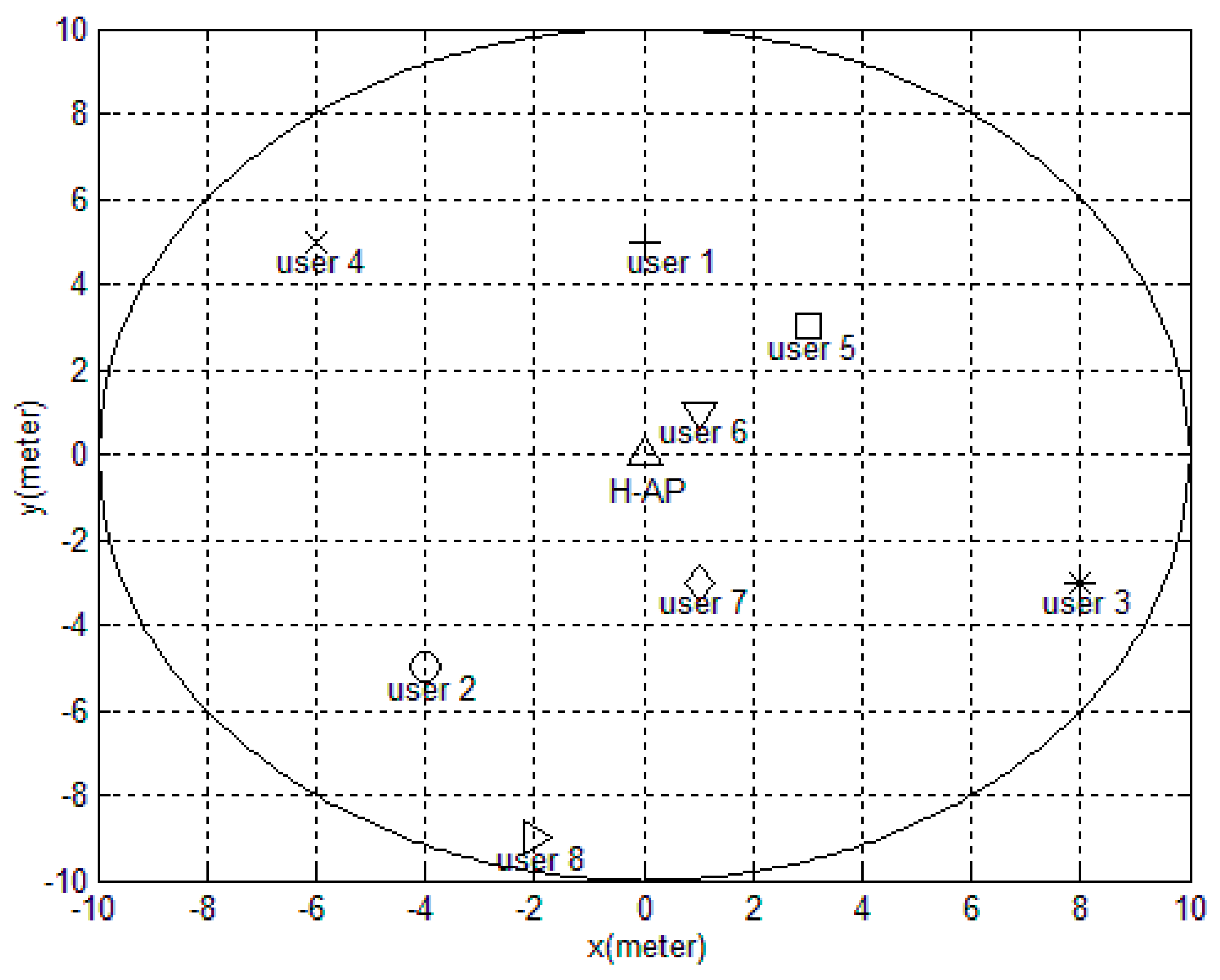
| Three-dimensional location of H-AP | (0, 0, 0) |
| Three-dimensional location of users | (0, 5, 0), (−4, −5, 0), (8, −3, −1), (−6, 5, 0), (3, 3, 1), (1, 1, 0), (1, −3, 0), and (−2, −9, 1) (m) |
| Distance from H-AP for user k | 4, 6.4, 8.6, 8.48, 4.36, 1.41, 2.24, and 9.27 (m) |
| Number of transmit antennas at the H-AP, M | 80 |
| Number of TS antennas for user k, | 16, 32 |
| Initial transmission power, | |
| Outage probability for C4 and C5, and | 0.15, respectively |
| Bandwidth for user k, | |
| Static circuit power dissipation at H-AP, | |
| Static circuit power dissipation at user k, | |
| Maximum transmission power, | |
| Maximum power supply from the power grid, | |
| 0.8 | |
| Target channel capacity, | |
| Target amount of harvested energy, | |
| Center frequency, | |
| Noise variance, | −119.23 (dBm) |
| Noise spectral density, | −174 (dBm/Hz) at 290 degree Kelvin. |
| Power inefficiency of the power amplifier, | 5 |
© 2017 by the authors. Licensee MDPI, Basel, Switzerland. This article is an open access article distributed under the terms and conditions of the Creative Commons Attribution (CC BY) license (http://creativecommons.org/licenses/by/4.0/).
Share and Cite
Hwang, Y.M.; Park, J.H.; Shin, Y.; Kim, J.Y.; Kim, D.I. Transmission Power and Antenna Allocation for Energy-Efficient RF Energy Harvesting Networks with Massive MIMO. Energies 2017, 10, 802. https://doi.org/10.3390/en10060802
Hwang YM, Park JH, Shin Y, Kim JY, Kim DI. Transmission Power and Antenna Allocation for Energy-Efficient RF Energy Harvesting Networks with Massive MIMO. Energies. 2017; 10(6):802. https://doi.org/10.3390/en10060802
Chicago/Turabian StyleHwang, Yu Min, Ji Ho Park, Yoan Shin, Jin Young Kim, and Dong In Kim. 2017. "Transmission Power and Antenna Allocation for Energy-Efficient RF Energy Harvesting Networks with Massive MIMO" Energies 10, no. 6: 802. https://doi.org/10.3390/en10060802
APA StyleHwang, Y. M., Park, J. H., Shin, Y., Kim, J. Y., & Kim, D. I. (2017). Transmission Power and Antenna Allocation for Energy-Efficient RF Energy Harvesting Networks with Massive MIMO. Energies, 10(6), 802. https://doi.org/10.3390/en10060802