Sizing Combined Heat and Power Units and Domestic Building Energy Cost Optimisation

Abstract

Many combined heat and power (CHP) units have been installed in domestic buildings to increase energy efficiency and reduce energy costs. However, inappropriate sizing of a CHP may actually increase energy costs and reduce energy efficiency. Moreover, the high manufacturing cost of batteries makes batteries less affordable. Therefore, this paper will attempt to size the capacity of CHP and optimise daily energy costs for a domestic building with only CHP installed. In this paper, electricity and heat loads are firstly used as sizing criteria in finding the best capacities of different types of CHP with the help of the maximum rectangle (MR) method. Subsequently, the genetic algorithm (GA) will be used to optimise the daily energy costs of the different cases. Then, heat and electricity loads are jointly considered for sizing different types of CHP and for optimising the daily energy costs through the GA method. The optimisation results show that the GA sizing method gives a higher average daily energy cost saving, which is 13% reduction compared to a building without installing CHP. However, to achieve this, there will be about 3% energy efficiency reduction and 7% input power to rated power ratio reduction compared to using the MR method and heat demand in sizing CHP.

1. Introduction

Combined heat and power (CHP) units are regarded as one of the most promising low carbon technologies in solving energy-related problems, because they have many advantages when compared with other energy generation technologies [1]. First, compared to conventional energy generation systems, CHP systems have much higher overall output efficiencies and because of that CHP units are installed to reduce carbon emission [2]. Secondly, in the case of renewable energy generation systems, climate change has less influence on CHP system control [3]. Moreover, the installation cost of a CHP unit is gradually decreasing. In [4], it is predicted that by the end of 2015 the capital cost of a CHP system will be around €374/kW. Similar to the prediction results shown in [4], the micro-CHP installation cost in 2016 is £300/kW [5]. Therefore, more micro-CHP units, whose output power is “kW level”, are being installed in domestic buildings.

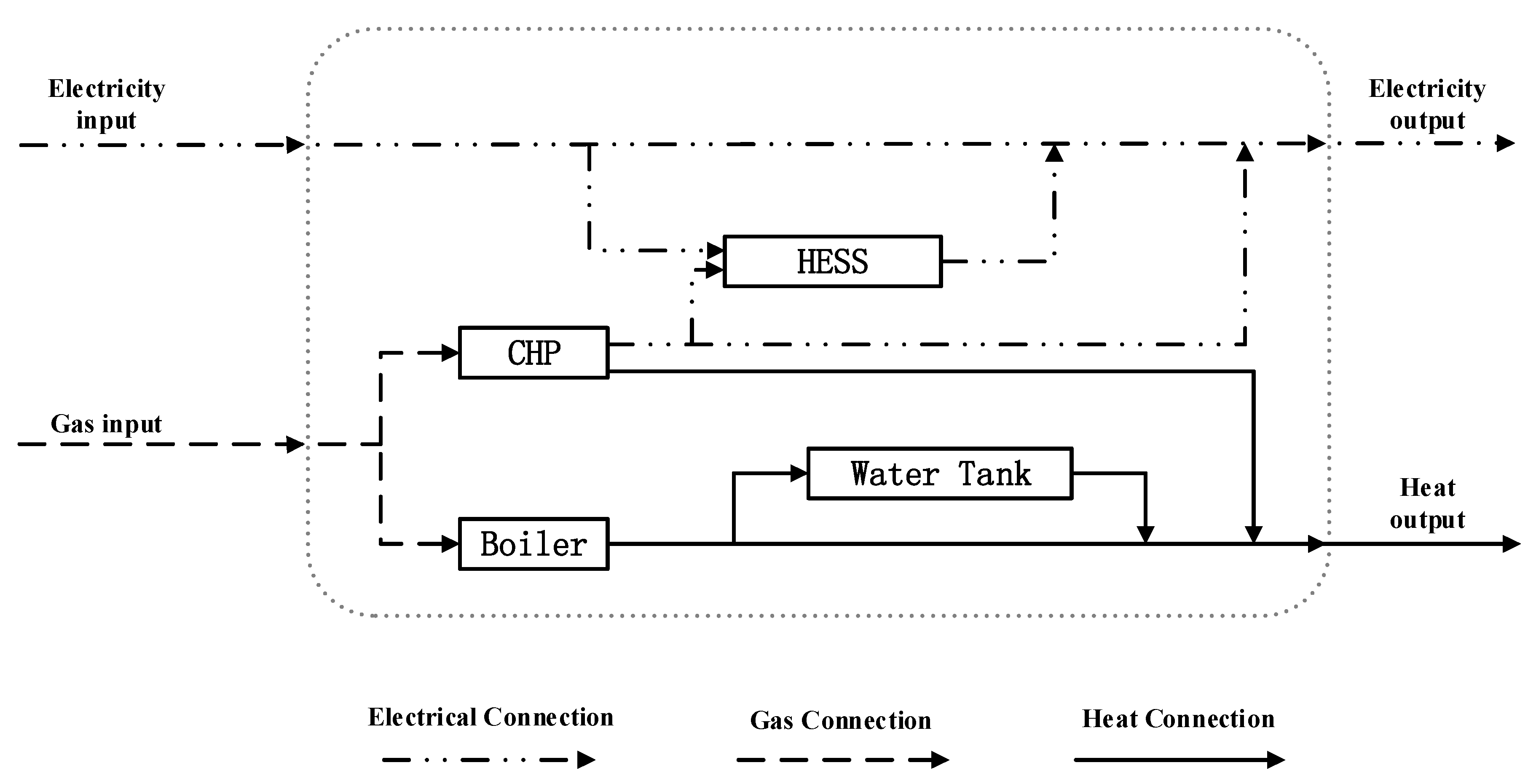
Batteries are still one of mature technologies to store electricity, and they can be used to improve energy system efficiency and to reduce carbon emissions; however, the installation cost and maintenance cost of a battery storage system are very high. Therefore, it is worth considering whether it is economical to install a battery storage system in a domestic building whose electricity load is supplied by a CHP unit and the grid and the heat load is supplied by a CHP unit and gas boiler. In this paper, battery storage systems are excluded.

Without an energy storage system, the key factors that can influence the daily energy costs and energy efficiency of aforementioned buildings are the capacity of CHP and the type of CHP [6]. Previous literature has already shown that the electricity output efficiency of micro-CHP is a quarter of its rated value when the CHP is operated at 10% of its rated power. Meanwhile, the heat output efficiency can also be reduced, if the CHP is working at low input power [1]. To increase energy efficiency and reduce emission, it is always preferable to have small capacity CHP in buildings. However, small scale CHP cannot meet the load at the peak demand time, even though it works at rated power. This will significantly increase the system’s daily energy costs. To reduce this cost, it is preferable to have large size capacity CHP. Thus, to improve both energy efficiency and system daily benefits, it is important to size CHP in domestic buildings.

To get an appropriate capacity of CHP, selecting sizing criteria is crucial, because optimisation results will differ depending upon the optimisation criteria used. Types of CHP and particular demand are two crucial criteria that are used to size the CHP. This paper considers two common types of CHP: gas engine and fuel cell. The main difference between these two CHP units is in output efficiency. Fuel cell CHP normally has a higher electricity to heat output efficiency ratio compared to gas engine CHP [7]. In [8], the rated electricity to heat output efficiency ratios for the fuel cell and gas engine CHP are about 33% and 74% respectively. In this paper, two types of CHP have been used as examples to optimise the size of CHP and the daily energy costs.

In domestic buildings, there are normally two types of demands: heat and electricity. As mentioned before, they can be used as another criteria to size CHP. This is because the heat and electricity consumption patterns in a domestic house are quite different from each other. In [4,9], using the heat demand curve to size and control the CHP is preferable, because CHP thermal output efficiency is normally greater than electricity, and in [4], it is assumed that the redundant electricity can be sold back to the grid. However, there are increasingly higher requirements to sell electricity back to the grid in Europe. For example, the European standard EN50160 states that the 10-min average root mean square voltage deviation should not exceed ±10% of the nominal voltage [10]. Considering this and the fact that many electricity meters do not have the ability to record electricity sent back to the grid, this paper assumes that there is no financial benefit from export, thus export is avoided.

There are many methods can be used to size a CHP and optimise system daily energy costs, for example the MR method, the GA method, the linear programming (LP) method and the nonlinear programming (NLP) method. Considering the fact that the LP method needs to linearise all constraints which can lead to loss of accuracy in the optimisation results, and the fact that NLP has trouble in distinguishing between the local minima and the global minimum, the MR, in this paper, will be used to optimise the size of a gas engine and fuel cell CHP for a domestic house, based firstly on the daily heat load and secondly on the electricity load curves. This is because the MR can cover an ‘average’ heat and electricity demand instead of covering the maximal heat or electricity demand, and thus can make full use of CHP capacity and improve CHP output efficiencies [4]. Because the GA is a powerful tool to deal with multivariable non-linear problems, the GA will be used to calculate the optimal daily operational cost. In the following work, two methods are used to find the best capacity of CHP and the theoretical minimum daily energy cost. The first one is the combination of the MR and the GA methods, which firstly optimises the CHP capacity by the MR method and then optimises the daily energy cost for the CHP capacity obtained by the MR method through the GA method. Another one only uses the GA method to find the optimal daily energy costs for different CHP capacity. By finding the theoretical minimum daily energy cost from the optimal daily energy costs, the best capacity of CHP can be acquired.

To reduce variables in the optimisation algorithms, [11] assumes that the CHP output efficiencies are constants for different operational conditions. However, this assumption gives a higher energy efficiency and a lower daily energy cost in optimisation results. In order to eliminate the impacts of this assumption, this paper uses the experimental results in [1] to formulate the CHP output efficiencies as functions that are only related to CHP input power. This will improve the accuracy of optimisation results and the output efficiencies of CHP.

The major contributions of this paper are: (1) two different sizing CHP methods (the MR and the GA) are used to find the optimal size of CHP. The computation time is significantly reduced by using the MR method and the optimal costs are lower when using the GA method; (2) The CHP output efficiencies are formulated to functions which are only related to input power and this gives a more accurate optimisation result compared to using constant CHP output efficiencies as optimisation criteria; (3) Different types of CHP and loads are considered as sizing criteria, and the optimisation results will give suggestions for engineers on how to choose and size CHP.

2. Optimisation Methodology

2.1. The Genetic Algorithm Method

The genetic algorithm (GA) method is a powerful and effective tool to deal with optimisation problems, and previous literature has proven that it is especially successful in solving single objective optimisation problems. Moreover, for multi-objective optimisation problems, the GA is intelligent enough to balance the trade-offs between each conflicting objective [12]. Compared with other optimisation algorithms, the GA method shows its strong ability of dealing with non-linear and non-continuous optimisation problems [13]. The GA can give highly accurate results, however, it normally needs a relatively long computation time.

There are four key factors of the GA: chromosomes (individuals), selection, crossover and mutation. By analogy to natural evolution, individuals are the solution candidates and each individual contains some variables. The set of individuals is called the population and the number of individuals in each population is population size. The selection process selects high-quality individuals and removes low-quality individuals. In this process, the GA defines a scale value called fitness, and this value can be used to show the performance of the optimisation results. Finally, crossover and mutation are the most important part of the GA. The crossover and mutation are used to generate new solutions within the search space. The offspring produced after the crossover and mutation will perform better in their environment due to higher fitness. The algorithm is terminated successfully when an individual emerges with an acceptably high fitness. In the following work, the population size, crossover fraction and generations (stopping criteria) are set as 20, 0.8 and 100, respectively. These parameters are default values of the GA in MATLAB optimisation toolbox (MATLAB 2010b, MathWorks Company, Natick, MA, USA). The reasons for choosing the GA in MATLAB optimisation toolbox are that it reduces programming time, and it also considers computation time and optimisation results coherently. As mentioned before, to get accurate results, the GA needs to take a longer computation time. However, this time is dependent on the generation and population size. Large and small generation and population size will reduce calculation efficiency.

2.2. The Maximum Rectangle Method

The maximum rectangle (MR) method is normally used to size the energy generation equipment in a power system [4,14]. Compared with other optimisation algorithms, the MR method focuses on finding the best capacity of an energy generator which can cover majority of energy consumption instead of covering the maximal demand.

To implement this method, load (electricity or heat) distribution curves normally need to be acquired in advance. Figure 1 is an example of the MR design method. By inserting the rectangles, the MR method tries to find the rectangle which has the maximum area. The width of the selected rectangle is the theoretical best capacity of generator.

As long as the load distribution curve can be formulated, this method can find the optimal generator capacity very quickly. Using the MR method to size generators always gives a higher benefit cost ratio to energy systems, because the MR method tries to find the energy generator’s capacity which can cover majority of energy consumption.

3. CHP Sizing and System Optimisation

In the following parts, Section 3.1 demonstrates how to size CHP by the MR method according to different sizing criteria. After obtaining the best CHP capacities for different sizing criteria, Section 3.2 shows how to use the GA method to optimise the daily energy cost. Similar to Section 3.2, Section 3.3 uses the same methodology (GA) to optimise the daily energy cost for different types of CHP and find the theoretical best CHP capacities for different CHP. In Section 3.4, effective CHP energy efficiency and average CHP input power to rated power ratio will be defined to test CHP efficacy performance.

3.1. Sizing CHP by the MR Method

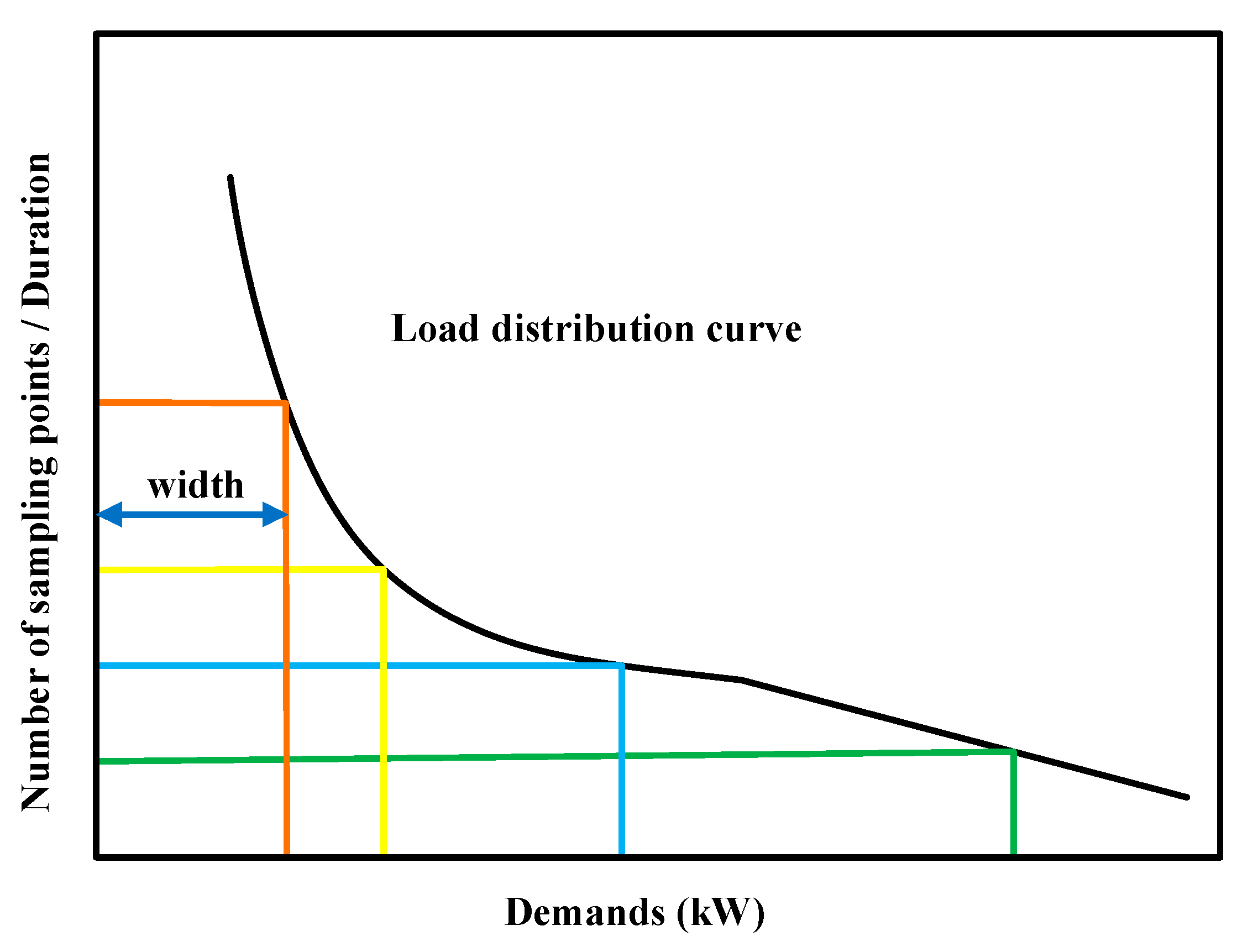
To use the MR method to size CHP based on electricity loads, five steps need to be taken. Firstly, recording every minute’s electricity demand in a year as sampling points is necessary. Secondly, the minimum and the maximum electricity demands in a year need to be found, and then equally divided into 10–20 intervals between maximum and minimum electricity demands. Too many intervals (more than 20) will cause the load distribution curve to fluctuate, and this will cause problems to formulate load distribution curves. On the other hand, few intervals (less than 10) will reduce the accuracy of curve fitting result. Therefore, 10–20 intervals between maximum and minimum electricity demands are needed. Thirdly, all sampling points need to be placed into related intervals and the number of sampling points in each interval must be calculated. The fourth step is to plot the load distribution curve as shown in Figure 1. Finally, based on the load distribution curve, sufficient rectangles need to be drawn as shown in Figure 1, and a rectangle which has the maximum area can be found. The demand (width) of this rectangle should be the capacity of CHP rated electricity output. At this step, the more rectangles that are plotted, the more accurate a result will be acquired.

3.2. Daily Energy Costs Optimisation by the GA Method

The daily energy cost objective function of a domestic building can be written as:

$$\mathrm{F}(\mathrm{t})={\displaystyle {\sum }_{\mathrm{t}=1}^{t=1440}{{\displaystyle P}}_{\mathrm{E}in}(t)\times }{{\displaystyle C}}_e(t)+{{\displaystyle P}}_{Gin}(t)\times {{\displaystyle C}}_g(t)+{{\displaystyle P}}_{CHPin}(t)\times {{\displaystyle C}}_g(t)$$

(1)

In Equation (1), F(t) is the daily energy cost in pence, C_e(t) and C_g(t) are the electricity price and gas price in each minute in a day respectively, and optimisation varibles P_Ein(t), P_Gin(t) and P_CHPin(t) are the imported average electrical energy from the grid, imported gas to supply the boiler and imported gas to supply the CHP in each minute respectively. To meet the electricity demand and heat demand in the building, the equality constraints can be generated as:

$${{\displaystyle P}}_E(t)={{\displaystyle P}}_{Ein}(t)+{{\displaystyle \eta }}_{CHPE}\times {{\displaystyle P}}_{CHPin}(t)$$

(2)

$${{\displaystyle P}}_{\mathrm{H}}(t)={{\displaystyle P}}_{\mathrm{G}in}(t)\times {{\displaystyle \eta }}_B+{{\displaystyle \eta }}_{CHPH}\times {{\displaystyle P}}_{CHPin}(t)$$

(3)

In Equations (2) and (3), P_E(t) and P_H(t) are the electrical energy demand and heat demand of the domestic building respectively in each minute. η_CHPE and η_CHPH are the CHP output electricity and heat efficiency respectively. η_B is the boiler’s gas to heat conversion efficiency. In addition, system limitations give extra inequality constraints which can be listed as follows:

$${{\displaystyle \eta }}_{CHPE\min }\le {{\displaystyle \eta }}_{CHPE}\le {{\displaystyle \eta }}_{CHPE\max }$$

(4)

$${{\displaystyle \eta }}_{CHP\mathrm{H}\min }\le {{\displaystyle \eta }}_{CHPH}\le {{\displaystyle \eta }}_{CHPH\max }$$

(5)

$${{\displaystyle P}}_{CHPin}(t)=0\mathrm{OR}\zeta \times {{\displaystyle P}}_R\le {{\displaystyle P}}_{CHPin}(t)\le {{\displaystyle P}}_R$$

(6)

$${{\displaystyle P}}_{Ein}(t)\ge 0$$

(7)

$${{\displaystyle P}}_{\mathrm{G}in}(t)\ge 0$$

(8)

Equations (4) and (5) describe the CHP electricity and heat output efficiency limitation. Equation (6) shows that a CHP unit can either be switched off or work at its feasible operational conditions. In Equation (6), P_R is rated/optimal power/capacity of CHP and ζ is a scaling factor. In [1], CHP input power can vary from 10% to 100% to its rated power. In this work, ζ is set as 10% and the optimal capacities acquired by the MR method will be used to find the daily optimal energy cost for each scenario. Equations (7) and (8) demonstrate that the electricity and heat can only be imported, not exported. In other words, they describe the direction of power flow.

As mentioned in the Introduction to this paper, both CHP heat and electricity output efficiencies decrease if CHP is working at low input power situations. In this work, CHP output efficiencies are formulated to functions which relate to CHP input power.

Table 1. Output efficiencies of the combined heat and power (CHP) for different input power [1].

Input Power/Rated Power (%)	Electricity Efficiency (%)	Heat Efficiency (%)
10	7.8	38.4
25	16.3	34.5
50	24.2	36.4
75	27.3	41.1
100	28.1	41.0

shows the efficiencies of the CHP for different CHP inputs, obtained from [1].

Based on Table 1, the electricity and heat output efficiencies of a general CHP unit can be formulated with the MATLAB curve fitting toolbox as follows:

$${{\displaystyle \eta }}_{\mathrm{CHP}E}={{\displaystyle \xi }}_E\times (11.67\times \log (\frac{{{\displaystyle P}}_{CHPin}(t)}{{{\displaystyle P}}_R})\times 100)-0.06459\times (\frac{{{\displaystyle P}}_{CHPin}(t)}{{{\displaystyle P}}_R})\times 100)-18.76)$$

(9)

$${{\displaystyle \eta }}_{\mathrm{CHPH}}={{\displaystyle \xi }}_H\times (0.1256\times (\frac{{{\displaystyle P}}_{CHPin}(t)}{{{\displaystyle P}}_R})\times 100)+82.32\times (\frac{{{\displaystyle P}}_R}{{{\displaystyle P}}_{CHPin}(t)})\times 100)+28.73)$$

(10)

In (9) and (10), ξ_E and ξ_H are the CHP electricity and heat output efficiency coefficients, and these values only relate to the type of CHP, or in other words, the design of CHP.

Table 2. Summary of gas engine and fuel cell CHP electricity and heat output efficiency coefficients.

Type of CHP	Electricity Output Efficiency Coefficients (ξE)	Heat Output Efficiency Coefficients (ξH)
Gas Engine	0.783	1.610
Fuel Cell	1.298	1.187

summarizes the electricity and heat output efficiency coefficients of the gas engine and the fuel cell CHP used in this paper.

3.3. Theoretical Best Capacity of CHP by the GA Method

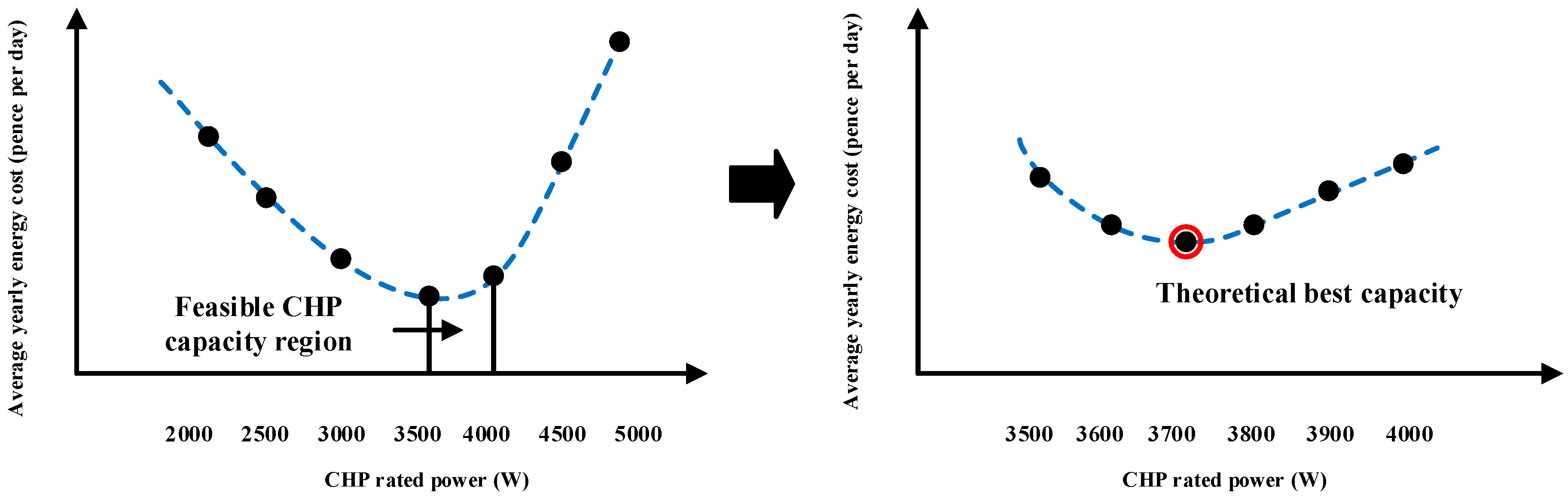
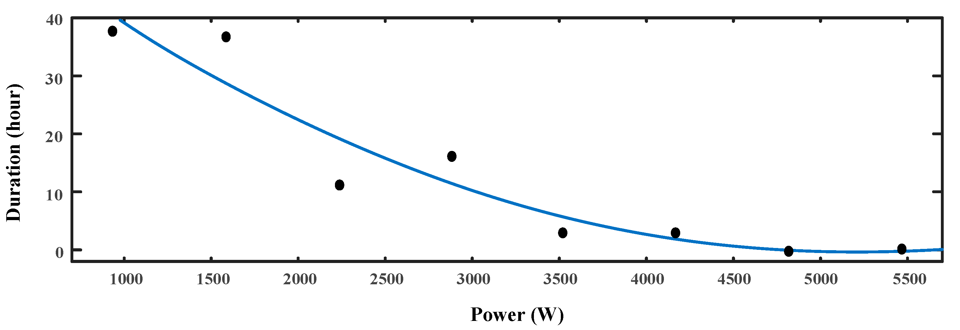
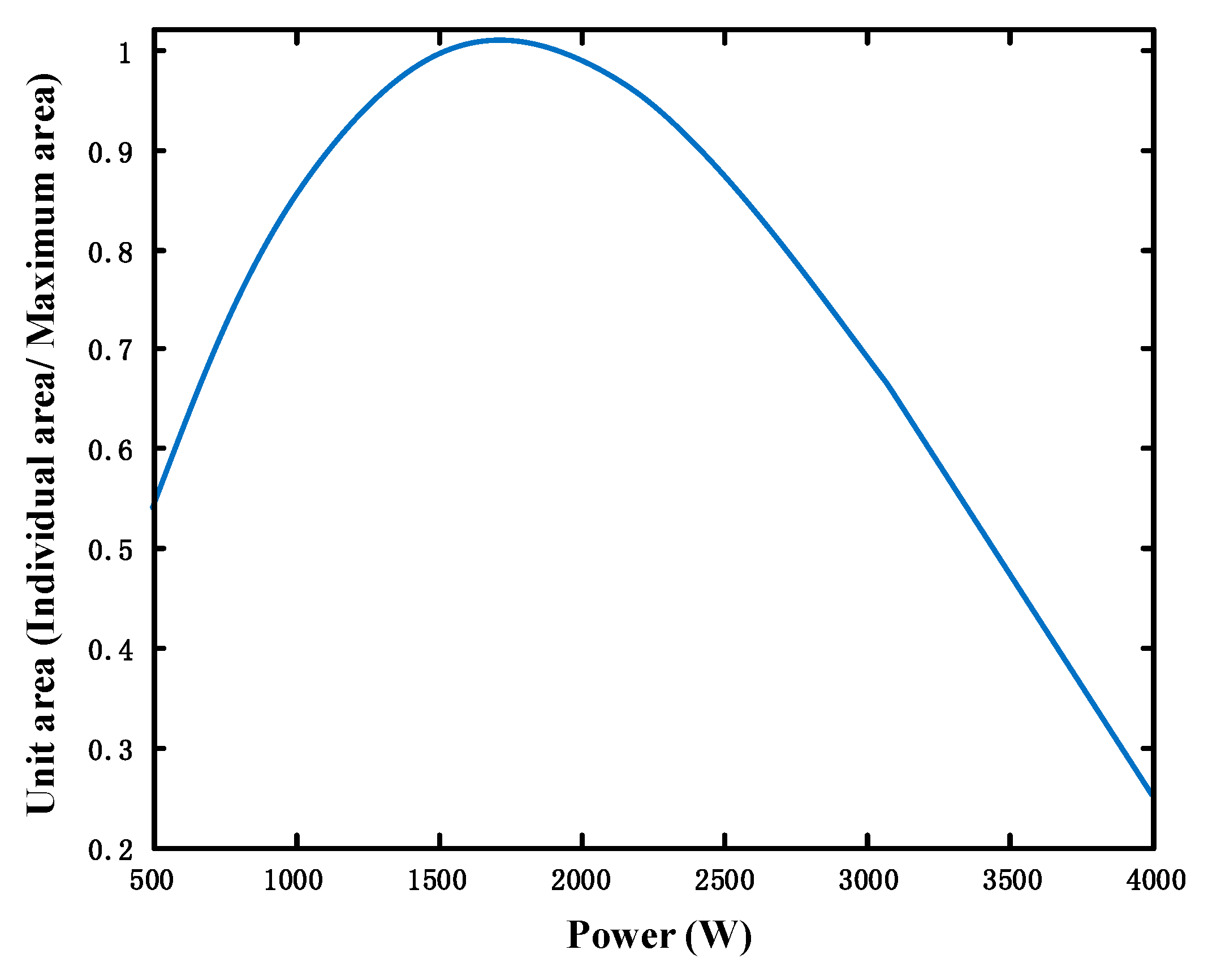
In this section, the GA method is used to optimise the daily energy costs for a system with different CHP installation capacities. Then, by comparing the daily energy costs for different CHP installation capacities, the theoretical best CHP capacity can be determined. However, considering the fact that the GA method normally takes a long computation time to get the optimisation results and that the output of commercial CHP units is normally quantified to 100 W, this work will calculate the best capacity of each type of CHP in discrete hundred Watt increments.

The daily energy cost functions, constraints and equations of this work are similar to Section 3.2. However, compared to Section 3.2, P_R will be treated as another new variable. This work will first find the feasible CHP capacity region and then find the best capacity of both type of CHP. The CHP output power will first be assumed to be 1000 W, and there will be 500 W increase every time until the output power of CHP reaches a point after which the daily energy cost will always increase with the increase of CHP capacity. At this stage, the GA method will be used to calculate the average daily energy cost for each CHP capacity. By plotting the rated capacity and average yearly energy costs graph, a feasible CHP capacity region can be acquired. Then the maximum and minimum capacity of this region is divided into five equal intervals, which means that four more samples need to be tested. By using the GA method to optimise daily energy costs of these four points, the theoretical best CHP can be acquired. Figure 2 shows this method.

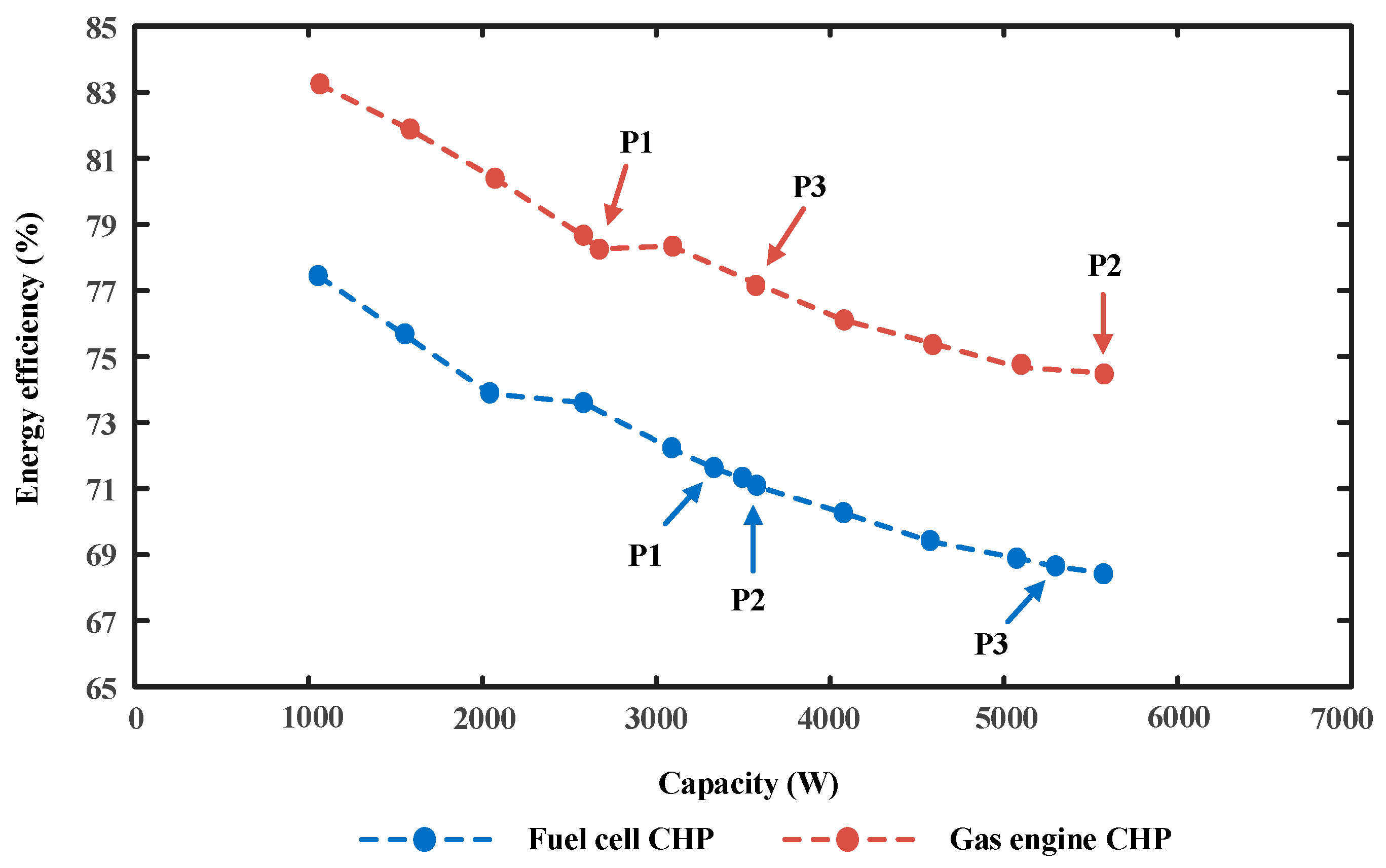
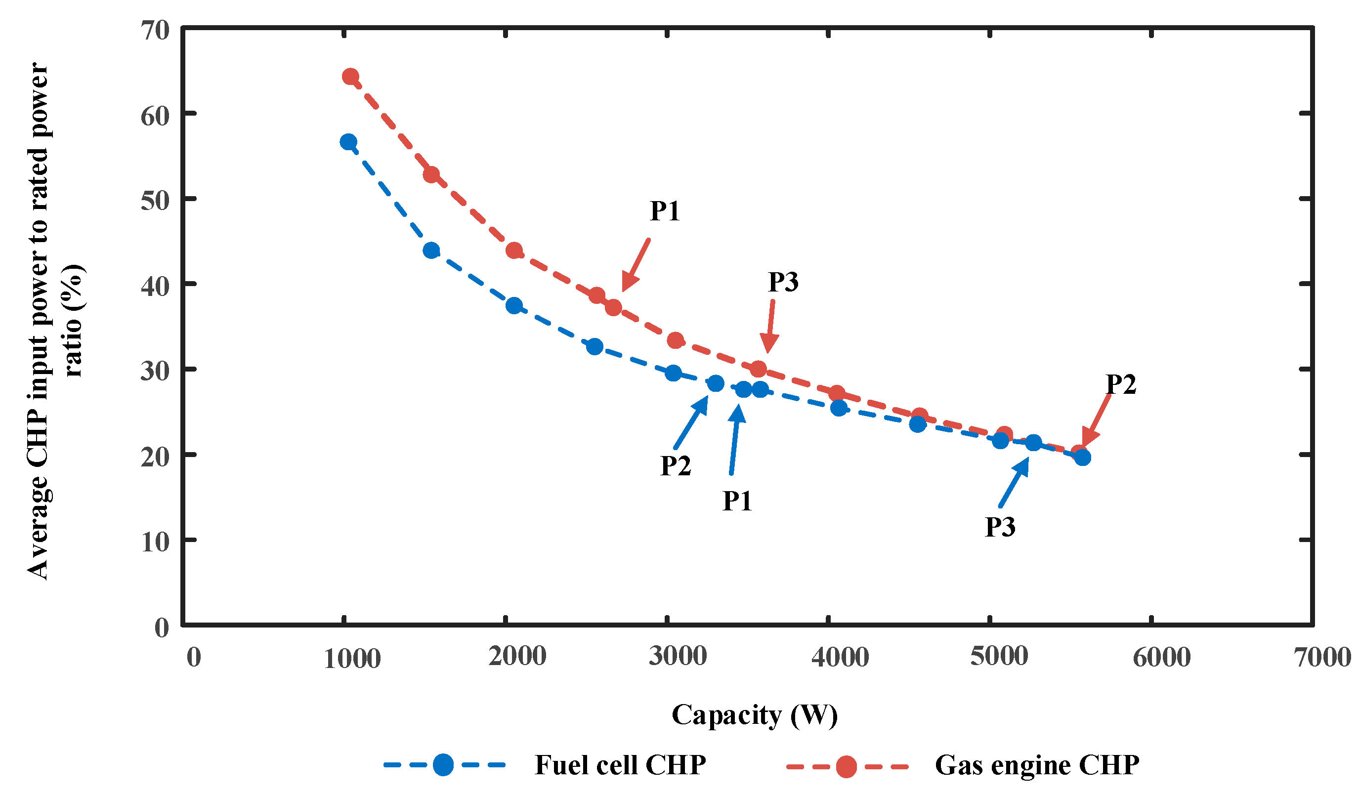
3.4. Effective CHP Energy Efficiency and Average CHP Input Power to Rated Power Ratio

As mentioned in the Introduction, CHP is a high output efficiency energy generator. However, system energy efficiency can be significantly reduced if an inappropriate capacity CHP unit is installed. Here, two parameters are defined to test the performance of CHP sizing results. First, the effective CHP energy efficiency is defined to calculate the average whole year CHP energy efficiency with different CHP capacities. Another parameter, average CHP input power to rated power ratio, is defined to illustrate whether the CHP is fully utilised. Equations (11) and (12) are the functions to show effective CHP energy efficiency and average CHP input power to rated power ratio:

$${{\displaystyle \tilde{\eta }}}_{\mathrm{CHP}}=\frac{{\displaystyle {\sum }_{t=1}^{\mathrm{t}=L}({{\displaystyle \eta }}_{CHPE}(t)+{{\displaystyle \eta }}_{CHPH}(t))}}{L^{\prime }},({{\displaystyle \eta }}_{CHPE}(t)+{{\displaystyle \eta }}_{CHPH}(t))>0$$

(11)

$${{\displaystyle h}}_{\mathrm{CHPH}}={\displaystyle {\sum }_{t=1}^{t=L}({{\displaystyle P}}_{CHPin}(t)/{{\displaystyle P}}_R)}/L^{\prime }$$

(12)

In (11), ῆ_CHP is effective CHP energy efficiency, η_CHPE(t) and η_CHPH(t) are the CHP electricity and heat output efficiency in tth minute respectively and L’ is the number of samples. In (11), both η_CHPE(t) and η_CHPH(t) should be greater than zero, because to calculate the effective CHP energy efficiency, the CHP switch off state should not be considered. In (12), h_CHP is the average CHP input power to rated power ratio.

4. Case Study

In this paper, a CHP system has been designed for a terraced domestic building in the UK of approximately 30 years in age, occupied by four people. In this building, there are two large single rooms, two large double rooms, a fixed size kitchen, a bathroom and a living room, which cover the total area of 152 m². Figure 3 shows the energy carriers and the layout of energy infrastructure in the building. Daily electricity consumption in this building was randomly generated by the CREST electricity model [15]. Daily heat consumption in this building was generated by the model developed by Strathclyde University [16]. The gas price is based on current UK domestic gas price which is around 5 pence/kWh, and the electricity tariff is obtained from [17], which proposes a dynamic system of tariffs which vary on a half hourly timescale. The daily electricity price in each 30 min for different seasons is shown in Figure 4.

5. Optimisation Results

5.1. CHP Sizing Results by the MR Method

The electricity demand distribution curve for the terraced house which was built approximately 30 years ago is shown in Figure 5. Figure 5 indicates that the electricity loads are less than 1 kW most of the time of during the year for this household.

After obtaining the electricity demand distribution curve, the rectangles can be drawn in the diagram. In this work, the width of rectangles increase 1 W per increment and the width of rectangles start at 300 W, and end at 3000 W. This is because from Figure 5, domestic CHP electricity demand is normally greater than 300 W and less than 3 kW. Figure 6 shows the area of the rectangles against different CHP electrical output power.

Figure 6 shows that when the electrical output of CHP is 1206 W, the rectangle will obtain the maximum area. Based on previous gas engine and fuel cell CHP heat and electricity efficiencies assumptions (shown in page 5), the heat output of gas engine and fuel cell CHP should be 3618 W and 1630 W, respectively. In other words, if the electricity load is used as a criterion to size CHP, the optimal rated capacity of gas engine and fuel cell CHP should be 5482 W and 3259 W respectively.

Figure 7 shows the heat demand distribution curve for the terraced house which was built approximately 30 years ago. From Figure 7, the domestic heat demand for a terraced house are less than 3 kW in most cases.

By applying the MR method to the heat demand distribution curve, the area of rectangles for different CHP output power is plotted in Figure 8.

Figure 8 indicates that by setting the rated heat output power of CHP as 1717 W, most of the heat demands can be supplied by the CHP during the year. Based on previous gas engine and fuel cell CHP heat and electricity efficiencies assumptions (shown in page 5), the capacity of electricity power for fuel cell CHP and gas engine CHP should be set as 1271 W and 571 W, respectively. Thus, if the heat demand is used as the criterion to size CHP, the optimal capacity of fuel cell CHP and gas engine CHP should be 3434 W and 2602 W.

Table 3. Optimal capacities of different types of CHP based on different types of loads.

Types of Loads	Types of CHP	Optimal Electrical Output of CHP (W)	Optimal Heat Output of CHP (W)	Optimal Rated Power of CHP (PR) (W)
Electricity	Gas Engine	1206	3618	5482
	Fuel Cell		1630	3259
Heat	Gas Engine	572	1717	2602
	Fuel Cell	1271		3434

is a summary of optimal capacities of different types of CHP based on different optimising criteria.

Table 3 shows that the optimal capacities of fuel cell CHP are nearly the same for this building, when either electricity loads or heat loads are chosen as optimising criteria. However, the optimal capacities of gas engine CHP can be significantly different when the heat load and the electricity load are used as optimising criteria. The result from Table 3 shows that the optimal capacity of electricity dependant sizing gas engine CHP is twice the capacity of heat dependant sizing gas engine CHP.

5.2. Daily Energy Costs Optimisation Results Based on Optimal CHP Capacity

By using the proposed methods in Section 3.1 and Section 3.2, the optimisation results (CHP output efficiencies and the average daily energy costs) of different seasons are shown in this section. Figure 9a–d show the CHP output efficiencies (including heat, electricity and overall efficiencies) in each minute of a typical CHP based on different seasons.

Figure 10 is a graph to show daily energy costs in different seasons based on different sizing criteria.

5.3. Theoretical Best CHP Capacity and Minimum Daily Energy Cost by the GA Method

This part shows the theoretical best fuel cell and gas engine CHP capacities based on the algorithm proposed in Section 3.3.

5.3.1. Theoretical Best Fuel Cell CHP Capacity

Figure 11 is a graph to show the relationship between fuel cell CHP installation capacity and average daily energy costs. Figure 11 reveals that the average daily energy cost for a year decreases with the increase of fuel cell CHP capacity until the CHP capacity reaching 5000 W. From Figure 11, the theoretical best fuel cell CHP capacity should be located between 5000 W and 5500 W. Figure 12 shows the average daily energy cost for different CHP installation capacities which are located within the feasible region. From Figure 12, the daily energy cost is at a global minimum when the capacity of the fuel cell CHP is set as 5200 W.

5.3.2. Theoretical Best Gas Engine CHP Capacity

Figure 13 is a graph to show the relationship between gas engine CHP installation capacity and average daily energy costs. Figure 13 indicates that the average daily energy cost for a year decreases with the increase of gas engine CHP capacity until the CHP capacity reaches 3500 W. From Figure 13, the theoretical best gas engine CHP capacity should be located between 3000 W and 3500 W.

Figure 14 is plotted to show the average daily energy costs for different CHP installation capacities which are located within feasible region. From Figure 14, the theoretical best gas engine CHP capacity is 3500 W. Compared with the MR method, the GA method gives a further 1.25 pence daily energy cost reduction and a nearly the same optimal gas engine CHP capacity.

The simulation results show that the fuel cell CHP and the gas engine CHP offer 13% and 8.4% of average daily energy cost reduction of a year compared to the building without installing CHP. This proves that fuel cell CHP has better performance in domestic energy cost reduction. However, to achieve the extra 4.6% energy cost reduction, the installation capacity of fuel cell CHP is 48.5% higher than gas engine CHP. Moreover, considering different manufacturing cost of two CHPs [8], the investment cost of fuel cell CHP will be 55.8% higher than gas engine CHP.

5.4. Effective CHP Output Efficiency and Average Input Power to Rated Power Ratio

Figure 15 and Figure 16 show the CHP installation capacity against effective CHP output efficiency and input power to rated power ratio, respectively. Both of graphs reveal that the effective CHP output efficiency and input power to rated power ratio reduce for both types of CHP when CHP installation capacity is increasing. In these two graphs, P1 and P2 are the theoretical best CHP capacity acquired by the MR method. The difference is that P1 uses the heat demand as sizing criteria and P2 uses the electricity demand as sizing criteria. P3 is the theoretical best CHP capacity acquired by the GA method.

Figure 15 shows that both CHP are operated at high output energy efficiency states for different CHP installation capacity. This is because that CHP is a kind of high energy efficiency generators. The graph also shows that gas engine CHP has higher effective energy efficiency compared to fuel cell CHP, the reasons being that heat demand is much higher than electricity demand in a domestic building and gas engine CHP rated energy efficiency is higher than fuel cell CHP.

Figure 16 indicates without an energy storage system, the capacity of CHP has not been fully utilised. For both CHP technologies, to get theoretical minimum daily energy cost, less than 30% of capacity is utilised.

6. Analysis and Discussion

Table 4. A summary of the optimal results based on different CHP sizing criteria.

Sizing Criteria	Type of CHP	Optimal Capacity (W)	Base Case Average Daily Energy Cost (pence)	Optimal Average Daily Savings (pence)	Effective Energy Efficiency (%)	Average CHP Input Power to Rated Power Ratio (%)	Average Daily Investment (pence)
Heat	Fuel Cell	3434	448	53	71.32	28.05	529
Electricity		3259		52	71.62	28.91	502
Theoretical Best Size		5200		58	68.73	21.39	801
Heat	Gas Engine	2602		36	78.4	38.2	349
Electricity		5482		31	74.56	20.4	735
Theoretical Best Size		3500		37	77.34	30.47	469
Average daily investment (pence) = (Total investment + maintenance fees) (pence)/CHP life (in days)

is a summary of the work in this chapter. The average daily investment in this table is calculated based on the installation costs of gas engine and fuel cell CHP showing in [8]. However, the installation costs of gas engine and fuel cell CHP showing in [8] are higher than the present CHP installation costs. This is because [8] shows CHP installation costs 7 years ago. With the development of the micro-CHP technology, the installation costs of micro-CHP have already been reduced.

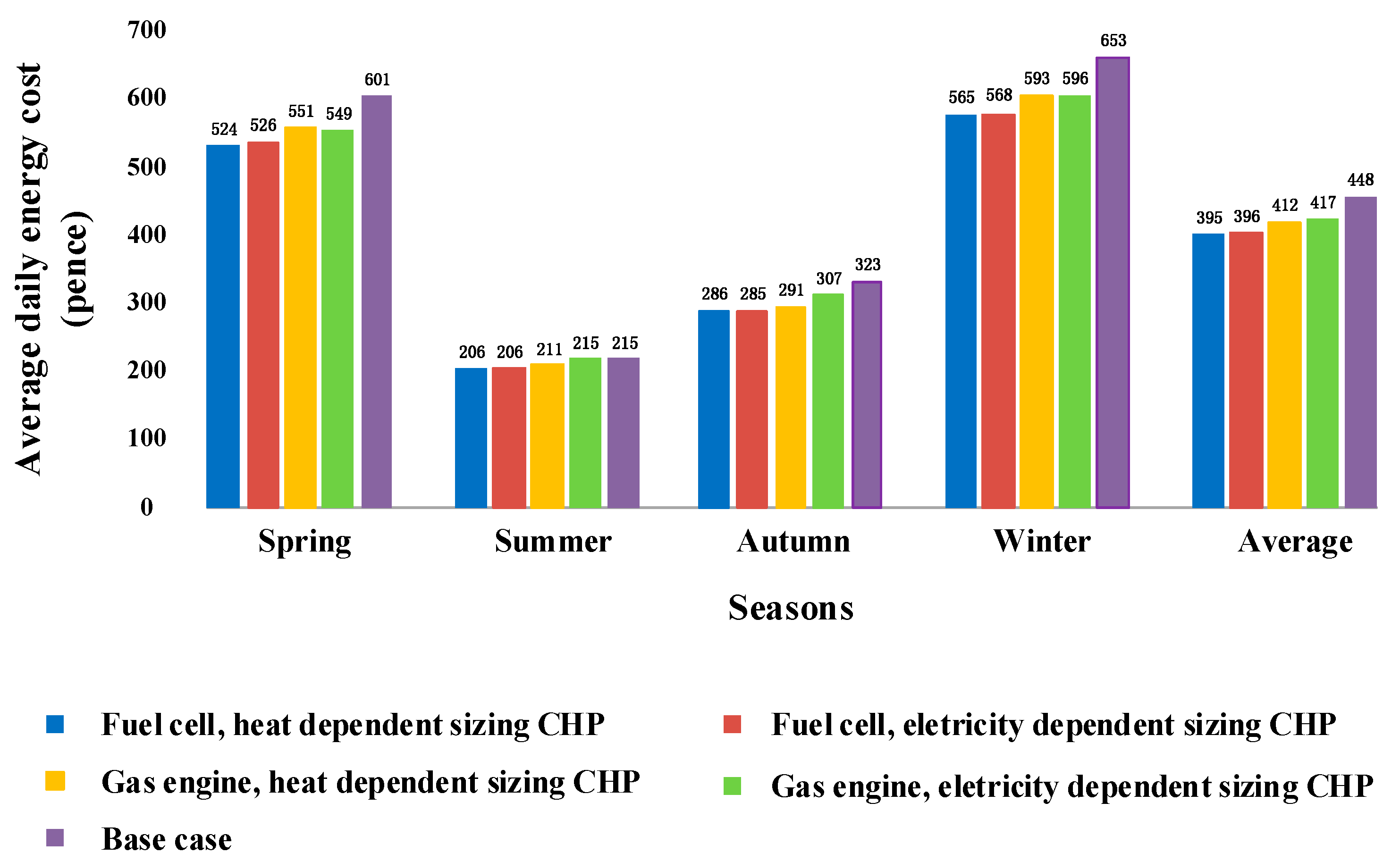
First, this work proves that using heat demand as optimisation criteria can obtain better optimisation results compared with electricity demand. This is because average heat demand in a year is much greater than the electricity demand. Only using the heat demand as sizing criteria to size fuel cell and gas engine CHP for a terraced house which was built approximately 30 years ago is acceptable, because compared with the theoretical best size CHP, the average daily energy savings are over 90% of theoretical maximum savings. However, using electricity as sizing criteria for gas engine CHP can cause problems, because the heat to power ratio of gas engine CHP is very high and this may cause the CHP to generate high levels of redundant heat.

Secondly, when using the MR method to size the CHP, the benefit to cost ratios are higher in most of cases compared to when the GA method is used to size the CHP. This is because the MR method tries to find the CHP capacity that can meet most of the demand in a year and this will make full use of CHP capacity. Consequently, even though the daily energy cost savings cannot achieve its theoretical maximum, the significant reduction of investment cost makes the ratio higher.

Thirdly, the optimisation results show that it is difficult to deal with the conflict between operational cost, system investment and energy efficiency. The optimisation results also show that to get higher daily energy savings, it is preferable to install large capacity CHP, however, this will significantly increase the investment cost and reduce energy efficiency. This is because by increasing the capacity of the CHP, more electrical demand occurring at the peak energy price time can be supplied by the CHP, and this will reduce energy costs. However, by increasing the capacity of the CHP, average CHP input power to rated power ratio is reduced, which means the CHP is always working at low input power and this will lead to energy efficiency reduction. Moreover, the low average CHP input power to rated power ratio indicates that most of CHP capacity has not been fully utilised. This is the reason why CHP investment cost is very high.

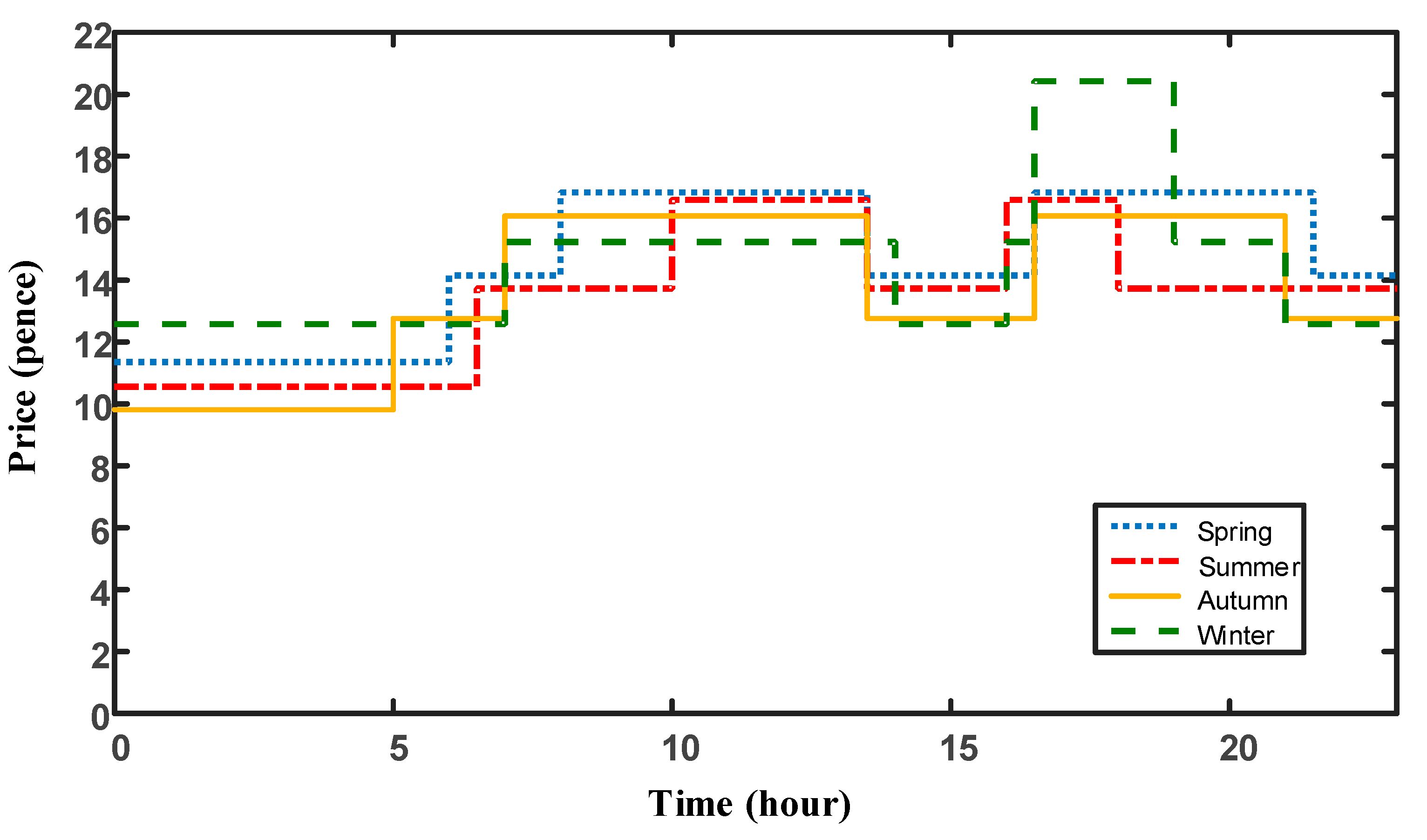
Fourthly, energy cost reduction is satisfactory in spring, autumn and especially winter. However, energy cost reduction in summer is disappointing. This is because the heat demand in summer is small compared with other seasons, therefore, the electricity generated by the CHP is limited. To increase energy cost reduction in summer, CHP capacity must be reduced, however, this can reduce energy cost reduction in other seasons. In order not to reduce energy cost reduction in other seasons, extra electrical energy must be stored in advance to supply the load at peak electricity price times.

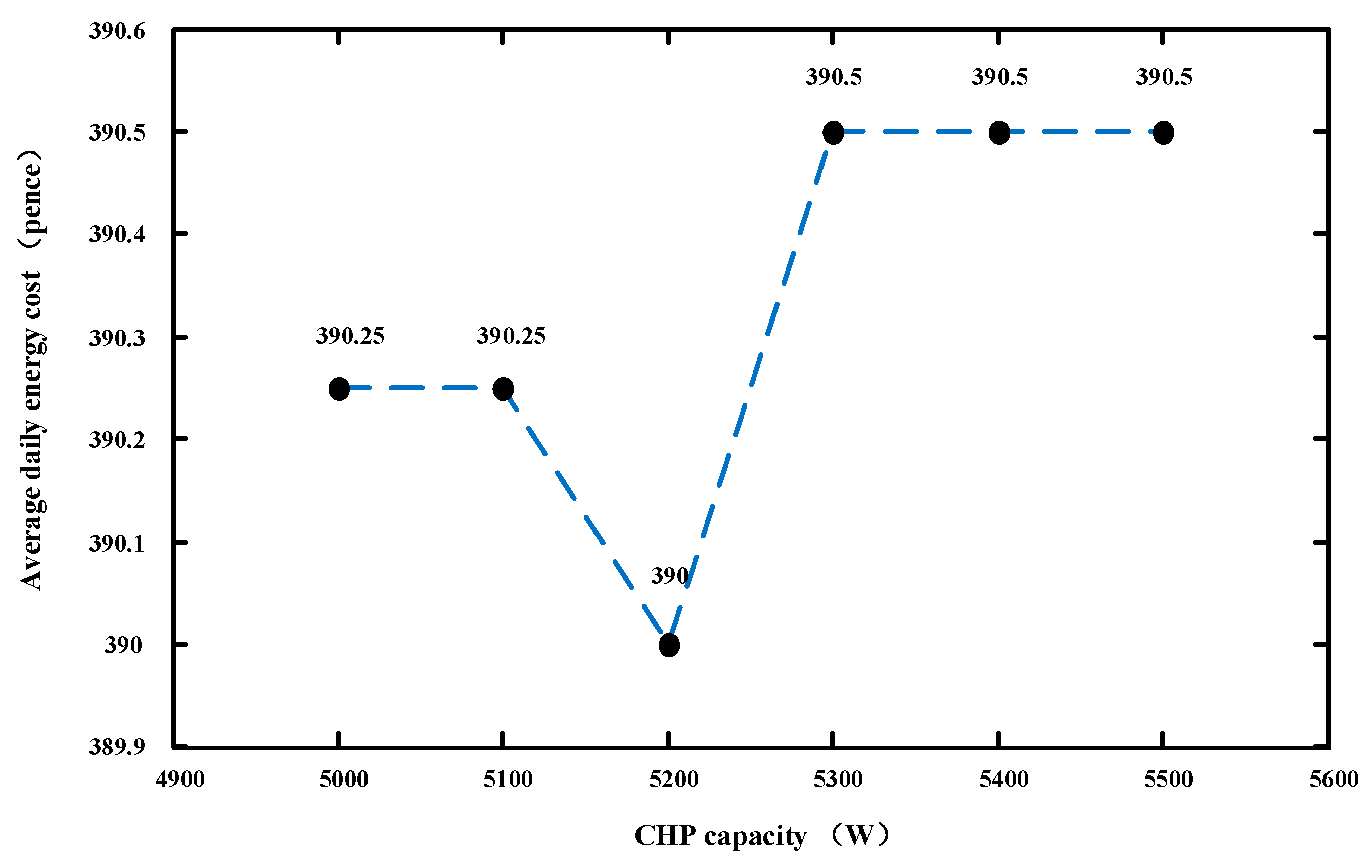
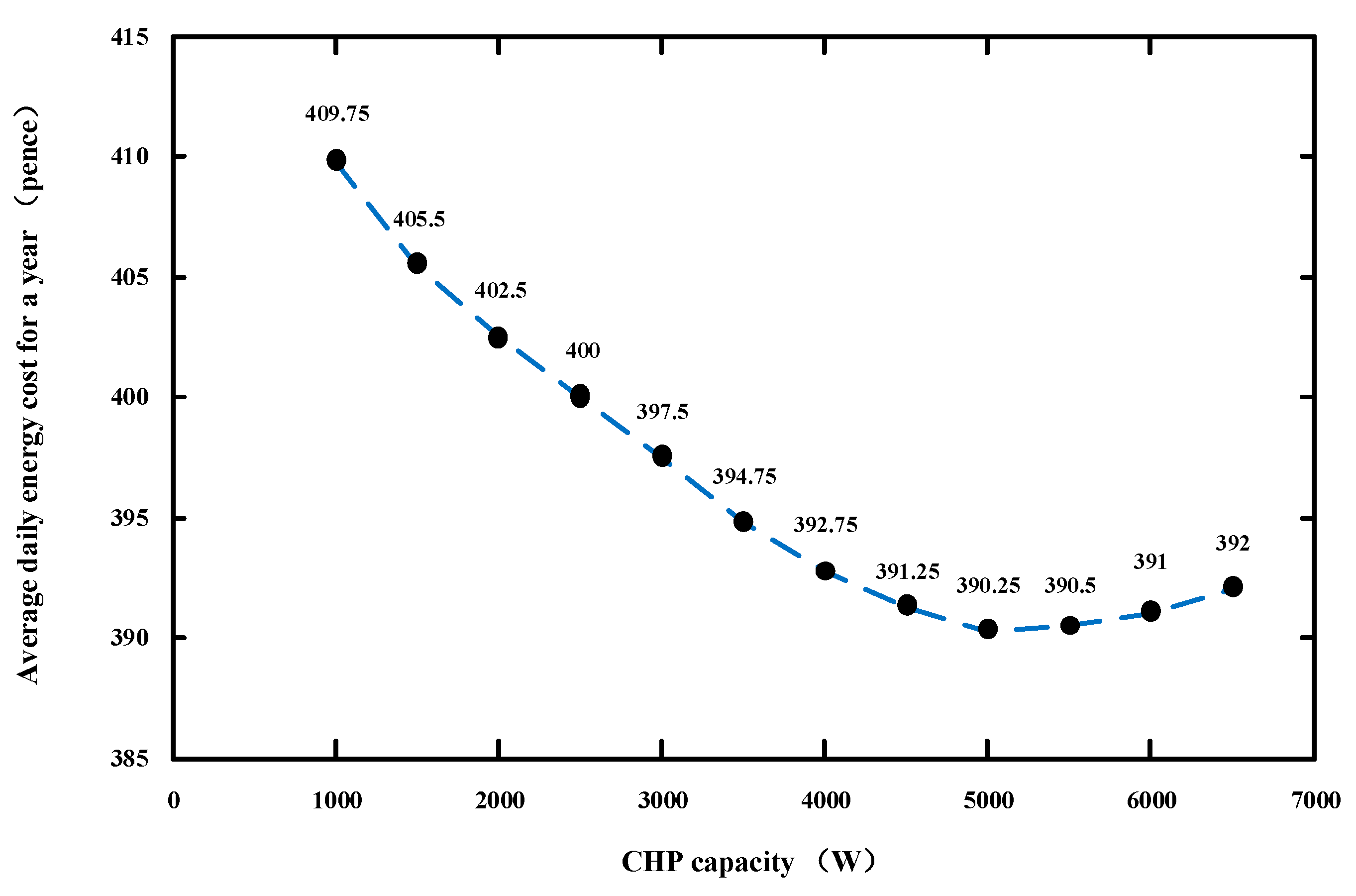
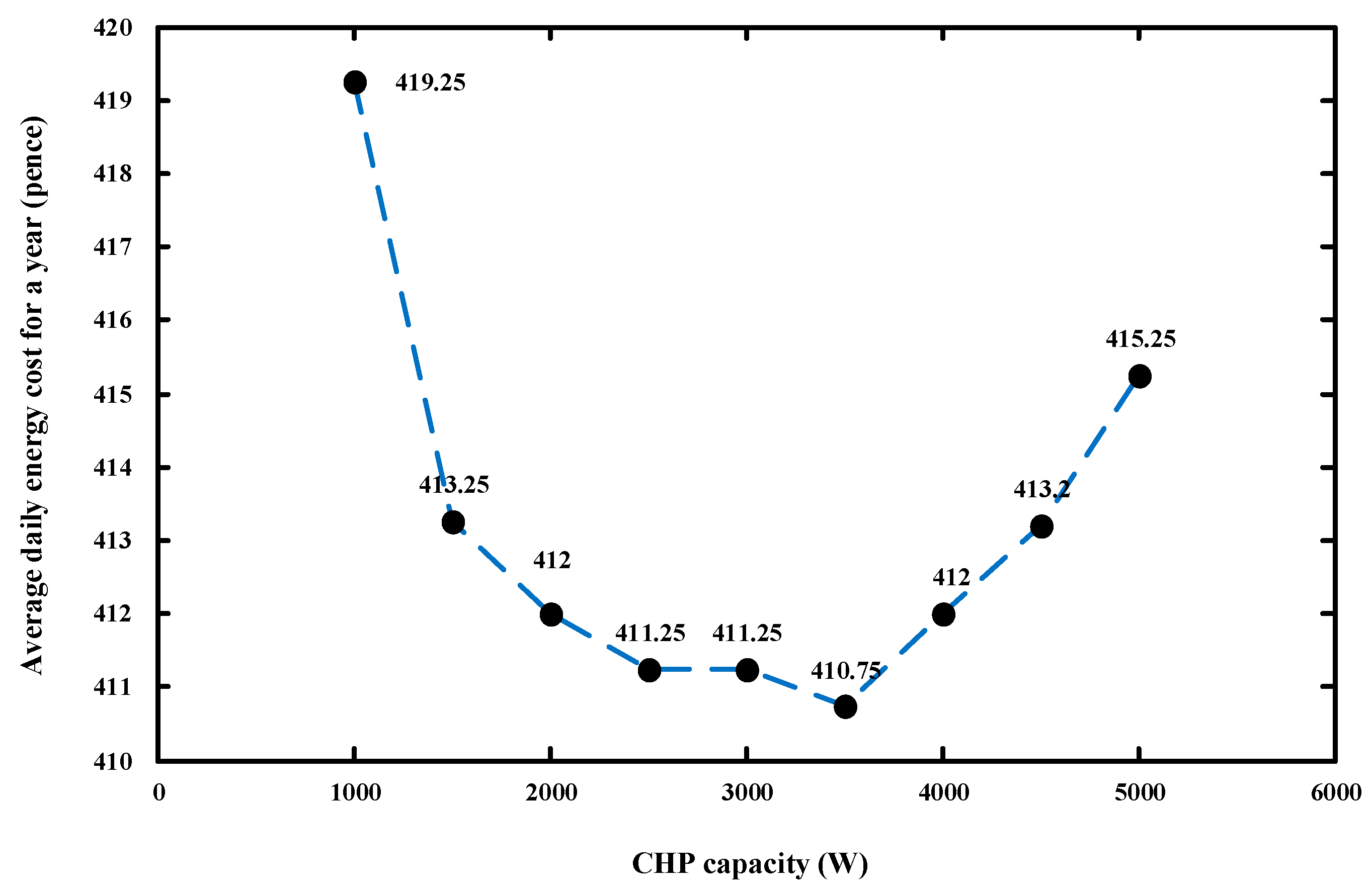
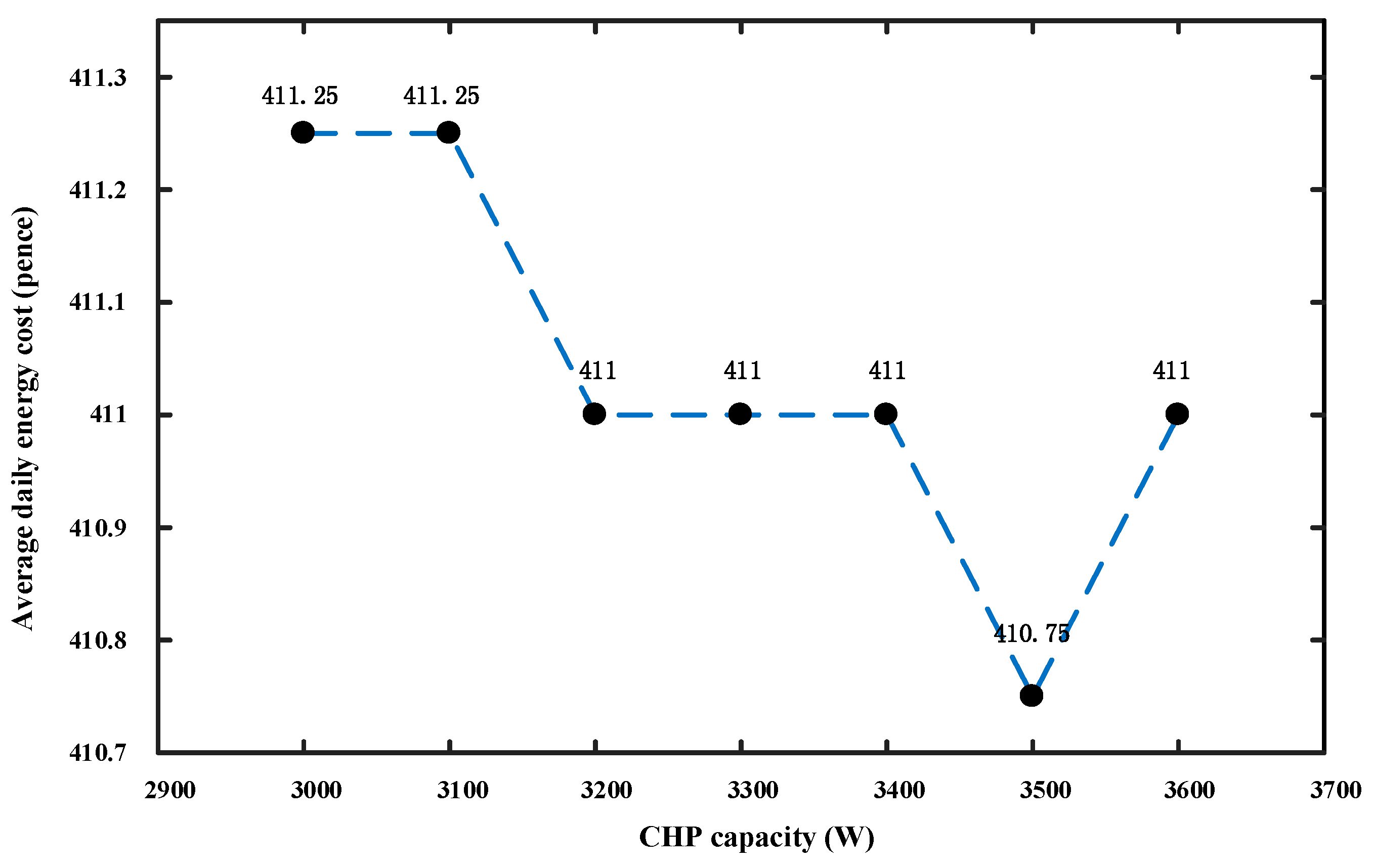
Finally, the results also show that the computation time of the MR method is much shorter than the GA method. The calculation time of the GA method normally depends on the scale of CHP capacity. Figure 10 and Figure 13 show that within the feasible CHP capacity region, the average daily energy costs are very similar, therefore, in the future work, the scale of CHP capacity in the GA method can be set as 500 W rather than 100 W and this will increase computation efficiency and reduce computation time.

7. Conclusions

This paper has shown that different optimization methods will lead to different optimization settings and that thermodynamics alone is insufficient for determining the best design point of CHP units. In this paper, daily energy operational costs, investment costs and energy efficiency are all considered when using the MR and GA methods to size the CHP. The GA optimisation results show that by installing a 5200 W fuel cell CHP, the daily energy costs can be minimized which is 13% reduction compared to base case. However, to achieve this reduction, there will be about 3% energy efficiency reduction and 7% input power to rated power ratio reduction compared to the use of the MR method and the heat demand to size CHP. Using the MR method and the heat demand to size the CHP is acceptable because the MR method gives a higher benefit to cost ratio and energy efficiency. In addition, it makes more use of CHP capacity, even though it needs 5 pence extra to generate energy for a day. Considering the fact that battery energy storage systems (BESS) and heat storage systems (HESS) are well suited to domestic buildings due to their relatively safe, silent, scalable, low maintenance, and efficient characteristics, BESS and HESS may need to be installed in the future to deal with the conflict between energy efficiency, energy costs and system investments if the installation cost of energy storage systems could be reduced.

References

1. Chen, X.P.; Wang, Y.D.; Yu, H.D.; Wu, D.W.; Li, Y.; Roskilly, A.P. A domestic CHP system with hybrid electrical energy storage. Energy Build. 2012, 55, 361–368. [Google Scholar] [CrossRef]
2. Jablko, R.; Saniter, C.; Hanitsch, R.; Holler, S. Technical and economical comparison of micro CHP systems. In Proceedings of the 2005 International Conference on Future Power Systems, Amsterdam, The Netherlands, 16–18 November 2005. [Google Scholar]
3. Tasdighi, M.; Ghasemi, H.; Rahimi-Kian, A. Residential microgrid scheduling based on smart meters data and temperature dependent thermal load modeling. IEEE Trans. Smart Grid 2014, 5, 349–357. [Google Scholar] [CrossRef]
4. Shaneb, O.A.; Coates, G.; Taylor, P.C. Sizing of residential μCHP systems. Energy Build. 2011, 43, 1991–2001. [Google Scholar] [CrossRef]
5. Energy International (UK) Limited, Commercial and Environmental Benefit Calculator 2016. Available online: http://www.energyinternational.co.uk/CHPCalculator1.htm (accessed on 26 April 2017).
6. Sheikhi, A.; Ranjbar, A.M.; Oraee, H. Financial analysis and optimal size and operation for a multicarrier energy system. Energy Build. 2012, 48, 71–78. [Google Scholar] [CrossRef]
7. Aki, H. The penetration of Micro CHP in residential dwellings in Japan. In Proceedings of the 2007 IEEE Power Engineering Society General Meeting, Tampa, FL, USA, 24–28 June 2007. [Google Scholar]
8. Ren, H.; Gao, W. Economic and environmental evaluation of micro CHP systems with different operating modes for residential buildings in Japan. Energy Build. 2010, 42, 853–861. [Google Scholar] [CrossRef]
9. Pehnt, M.; Cames, M.; Fischer, C.; Praetorius, B.; Schneider, L.; Schumacher, K. Micro Cogeneration: Towards Decentralized Energy Systems; Springer: Berlin, Germany, 2006. [Google Scholar]
10. Tant, J.; Geth, F.; Six, D.; Tant, P.; Driesen, J. Multiobjective battery storage to improve PV integration in residential distribution grids. IEEE Trans. Sustain. Energy 2013, 4, 182–191. [Google Scholar] [CrossRef]
11. Huber, M.; Sanger, F.; Hamacher, T. Coordinating smart homes in Microgrids: A quantification of benefits. In Proceedings of the 2013 4th IEEE/PES Innovative Smart Grid Technologies Europe (ISGT EUROPE), Lyngby, Denmark, 6–9 October 2013. [Google Scholar]
12. El Ela, A.A.A.; Ej-Din, A.Z.; Spea, S.R. Multi-objective genetic algorithm to improve the power system operation using distributed generation. In Proceedings of the 2006 Eleventh International Middle East Power Systems Conference, El-Minia, Egypt, 19–21 December 2006; pp. 612–619. [Google Scholar]
13. Kayo, G.; Ooka, R. Building energy system optimizations with utilization of waste heat from cogenerations by means of genetic algorithm. Energy Build. 2010, 42, 985–991. [Google Scholar] [CrossRef]
14. Haeseldonckx, D.; Peeters, L.; Helsen, L.; D’haeseleer, W. The impact of thermal storage on the operational behaviour of residential CHP facilities and the overall CO2 emissions. Renew. Sustain. Energy Rev. 2007, 11, 1227–1243. [Google Scholar] [CrossRef]
15. Richardson, M.T.I.; Infield, D.; Clifford, C. Domestic electricity use: A high-resolution energy demand model. Energy Build. 2010, 42, 1878–1887. [Google Scholar] [CrossRef]
16. Steemers, K.; Yao, R. A method of formulating energy load profile for domestic buildings in the UK. Energy Build. 2005, 37, 663–671. [Google Scholar]
17. Zhimin, W.; Chenghong, G.; Furong, L.; Bale, P.; Hongbin, S. Active demand response using shared energy storage for household energy management. IEEE Trans. Smart Grid 2013, 4, 1888–1897. [Google Scholar]
Figure 1. An example of the maximum rectangle (MR) design method.
Energies 10 00771 g001
Figure 2. Using the GA method to find the theoretical best CHP capacity.
Energies 10 00771 g002
Figure 3. Energy flow in smart building.
Energies 10 00771 g003
Figure 4. Daily electricity price in different seasons [17].
Energies 10 00771 g004
Figure 5. The electricity demand distribution curve for the terraced house which was built approximately 30 years ago.
Energies 10 00771 g005
Figure 6. The area of rectangles for different CHP electrical output power.
Energies 10 00771 g006
Figure 7. The heat demand distribution curve for the terraced house which was built approximately 30 years ago.
Energies 10 00771 g007
Figure 8. The area of rectangles for different CHP heat output power.
Energies 10 00771 g008
Figure 9. CHP output efficiencies in each minute of a spring day based on different sizing criteria. (a) Spring, fuel cell CHP, heat dependant sizing CHP; (b) Spring, fuel cell CHP, electricity dependant sizing CHP; (c) Spring, gas engine CHP, heat dependant sizing CHP; (d) Spring, gas engine CHP, electricity dependant sizing CHP.
Energies 10 00771 g009
Figure 10. Different daily operational costs based on different optimising criteria.
Energies 10 00771 g010
Figure 11. Average daily energy costs of a terraced house for installing different capacities fuel cell CHP.
Energies 10 00771 g011
Figure 12. Average daily energy costs within theoretical best fuel cell CHP capacity region.
Energies 10 00771 g012
Figure 13. Average daily energy costs of a terraced house for installing different capacities gas engine CHP.
Energies 10 00771 g013
Figure 14. Average daily energy costs within theoretical best gas engine CHP capacity region.
Energies 10 00771 g014
Figure 15. Effective CHP energy efficiency against CHP installation capacity.
Energies 10 00771 g015
Figure 16. Average CHP input power to rated power ratio against CHP installation capacity.
Energies 10 00771 g016