Abstract
Charging station location decisions are a critical element in mainstream adoption of electric vehicles (EVs). The consumer confidence in EVs can be boosted with the deployment of carefully-planned charging infrastructure that can fuel a fair number of trips. The charging station (CS) location problem is complex and differs considerably from the classical facility location literature, as the decision parameters are additionally linked to a relatively longer charging period, battery parameters, and available grid resources. In this study, we propose a three-layered system model of fast charging stations (FCSs). In the first layer, we solve the flow capturing location problem to identify the locations of the charging stations. In the second layer, we use a queuing model and introduce a resource allocation framework to optimally provision the limited grid resources. In the third layer, we consider the battery charging dynamics and develop a station policy to maximize the profit by setting maximum charging levels. The model is evaluated on the Arizona state highway system and North Dakota state network with a gravity data model, and on the City of Raleigh, North Carolina, using real traffic data. The results show that the proposed hierarchical model improves the system performance, as well as the quality of service (QoS), provided to the customers. The proposed model can efficiently assist city planners for CS location selection and system design.
1. Introduction
1.1. Motivation
The transportation sector has been one of the main sources of greenhouse gas (GHG) emissions and the primary driver of energy consumption: 26% of GHG emissions and almost one-third of the total energy in the United States originates from transportation [1]. Pushing electric vehicles (EVs) on the road is a potential way to reduce the GHG emissions and to lower the dependency on oil as the main energy source. Even though countries have set ambitious EV adoption goals over the last decade (e.g., one million EVs in the US by 2015), the use of EVs is still modest and almost all penetration targets have failed since 2010. Nevertheless, the cumulative EV sales have surpassed one million globally in 2016 and EVs constitute about 1% of the total light-duty fleet [2].
To understand consumer views on EVs, Ref. [3] presents a comprehensive field survey and identifies initial battery cost, limited battery range, and the lack of charging stations (CSs) as the main obstacles for acquiring an EV. Recent research and development activities have decreased the battery cost more than twofold and the unit cost dropped to 120 USD/kWh [4]. In addition to constant advances in the battery technology, governments offer incentive programs to reduce the cost of ownership to make EVs cost-competitive against the gas-powered counterparts. For instance, tax exemptions and access to easy parking options in Norway boosted the share of total EV registrations to 40% in 2016 [5]. On the other hand, to beat limited battery range the widespread presence of CSs is essential. Mainstream EVs can drive around 100 miles with a full battery, while some consumer surveys show that 300 miles of driving range is desired by the majority of consumers [3]. To bridge the gap between the current battery technology and the desired charging range, the deployment of a well-planned charging network is crucial.
In 2015, the number of public slow charging outlets (PSCOs) (which typically uses to kW) has reached 162,000, while the number of public fast charging outlets (PFCOs) (power rating 50 kW or more) has reached 28,000 [4]. Specifically, China and Japan possess 44% and 22% of the PFCOs worldwide [6]. However, the present deployment numbers are not sufficient to serve all EVs. On the global scale, an average of 7.8 EVs shared one PSCO and nearly 45 EVs shared a single PFCO in 2015. In countries like the United States, Canada, Norway, and France, approximately 90 EVs shared only one PFCO [4]. To address this issue, the US is building 48 new charging corridors on the national highways that will allow coast-to-coast travel.
An important feature of the CS networks is that the charging durations should be as short as possible. This is of utmost importance if EVs are to be competitive against the gas-powered vehicles. Hence, fast charging stations (FCSs) are likely to dominate the public charging grids to promote EV adoption. The ramifications of the CS deployment are long-lasting and impact various operational decisions. For the case of fast charging facilities, high costs associated with land acquisition, electrical equipment, energy storage systems, and facility construction make such siting projects long-term investments. Moreover, the current system state, e.g., vehicle distribution, customer routes between points of interests, population shift, etc., may change in the future. Therefore, finding robust station locations is a challenging job, which needs to incorporate uncertain future events. In this study, we propose a hierarchical optimization model to optimally locate a given number of FCSs in a region with the following objectives. The first one is to deploy the FCSs in a way that captures the maximal amount of traffic. The second objective is to find the best allocation scheme, in the sense of avoiding overload and under-utilization, for the limited number of PFCOs. The last objective is maximizing the system profit with the consideration of battery degradation costs and charging characteristics.
1.2. Related Work
The literature on EV CS location problem is growing in recent years. Refs. [7,8,9,10,11] analyzed the CS locations and scheduling of charging service from the system planning and the demand forecasting standpoints. In particular, the work in [7] proposed a predictive model for the development trend of EVs and CSs. The authors in [8] presented a simulator to analyze the location of CSs and the number of EVs charged at every service node. The analysis of charging demand, charging technology, and factors influencing the layout of CSs was presented in [9]. The work in [10] developed an interactive user application for charging slots allocation developed on structured query language (SQL) and hypertext preprocessor (PHP) platforms. The real-time forecast model provided the information of the availability of charging slots. The authors in [11] presented the factors of influencing load patterns and proposed methods for load forecast in the power system from the viewpoint of power system operator. On another hand, the literature also contains papers studying EV CS location problem based on classical facility location problems [12]. For the case of slow chargers, the siting problem typically aims to minimize a certain objective(s) such as minimizing the number of required chargers such that all customers can access a station within a predefined driving distance (set covering problem). For example, the study in [13] solved a set covering problem to minimize the number of CSs in California. If the budget for the chargers is fixed, then the goal could be to maximize the percentage of customers that can be served with a fixed number of them (maximum covering problem). The objective can also be the minimization of the maximum driving distance with P stations (P-center problem) [12,14]. For instance, the work in [15] presents an optimization problem to locate slow chargers in the City of Seattle, WA. A similar approach is used in [16], in which the objective is to minimize the construction cost by finding optimal locations for charging nodes. Due to the non-deterministic polynomial-time (NP)-Hardness of the proposed problem several approximate algorithms are developed.
The case for FCSs differs from the parked-based slow charging case, as the vehicles are mobile and they commute from one location to another. Therefore, flow-capturing models are more suitable. In them, the road network is represented using a graph. Furthermore, origin-destination (OD) pairs are defined for two nodes in the graph and the complete traffic flow is represented using a set of OD pairs. A vehicle commuting between an OD is assumed to be “captured” (or charged) if there is at least one facility located along the shortest path between this OD pair. A handful of studies have presented models for the optimal locations of the facilities to capture traffic flows [17,18,19,20,21]. The authors in [17] proposed a flow-capturing location allocation model (FCLM) to maximize the number of served customers. A gravity spatial interaction model was used to obtain the amount of traffic in every path. The authors in [18] proposed a model for the location of alternative-fuel stations, where every station has a limited capacity. In [19], a model named flow refilling location model (FRLM) was proposed to maximize the captured flow volume while considering the range of the vehicles. Moreover, the same group of authors presented an effective mixed-binary-integer programming formulation to solve the FRLM [20]. Applying the FCLM mentioned above, the authors in [21] presented two optimization models of FCS locations and illustrated its effectiveness on a case study of the City of Barcelona. However, most of the early works assume that a vehicle is charged when it passes through a located station. The model proposed in this paper adopts a queuing model and uses the charging duration as an important design parameter.
The underlying dynamics of the power distribution networks also play a critical role. Several studies proposed placing chargers at parking lots and locating stations by taking the limitations of power systems such as power losses, network reliability, and voltage deviations, into account [22,23,24,25,26]. The study in [22] proposed a resource allocation method of EV parking lots, with the consideration of the network reliability. The work was implemented on the Roy Billinton Test System (RBTS) bus 2. In [23], authors presented a two-stage model to minimize the system costs in the allocation of parking lots by considering the power losses and the network reliability at distribution feeders. In [24], a method for concurrent allocation of EV parking lots and the distributed renewable resources was proposed. Both the benefits of parking lot investor and the network operator were considered. The authors in [25] proposed a multi-objective optimization framework for the siting and the sizing of CSs for the distribution network expansion. Apart from allocating chargers at parking lots, the work in [26] presented methods for optimally placing CSs in the power network to maintain the reliability of the system. Particle Swarm Optimization (PSO) and Genetic Algorithm (GA) were utilized in the proposed methods. Different from the mentioned CS location models in the power distribution networks, the authors in [27] analyzed the influence of power quality from vehicle-to-grid (V2G) service and various different cases were performed for the evaluation.
Stochastic CS design was considered in [28,29,30,31,32,33,34]. In such studies, the system performance is usually measured by the average waiting time or the probability of getting blocked. The station design parameters include the amount of power drawn from the grid and the size of the energy storage device, if deployed. The work in [28] presented a spatial and temporal model for the EV charging demand at the CSs based on the traffic flows, where each CS was modeled as an queuing system. The study in [29] presented a BCMP queuing model to obtain the EV charging demands based on the stationary distribution of the number of EVs in each CS. The authors in [30] proposed a capacity planning framework for the CSs, which considered the multi-class customers and modeled each CS to be a queuing system. The capacity planning frameworks aimed to provide a certain level of quality of service (QoS) to EVs, where the blocking probability was selected as the QoS metric. The study in [31] proposed a model to solve the problems of sitting and sizing of CSs, considering the power distribution and transportation networks. In the capacity planning of the CSs, each CS was modeled as an queuing system and the maximum waiting time was used as the threshold for deciding the number of charging outlets in every CS. The work in [32] proposed a data-driven approach for an electric taxi CS sitting problem and an queuing model for the CS sizing problem in the city of Changsha, where the maximum block rate was adopted as a threshold. A model for the optimal electric bus CS capacity and bus charging schedule was presented in the study [33]. In [34], a quick-charging strategy was proposed for multi-type EVs in the highway CS design. Specifically, a power distribution model and a queuing model of CS were presented to reduce the waiting time and charging time of customers.
In this paper, we propose a hierarchical optimization framework to locate FCSs in a given city or highway network. Extended from the classic FCLM, the limited power supply, charging duration and the characteristics of battery model are considered in our model, which are crucial design parameters. First, we solve the flow capturing location problem to identify the locations of the CSs. Second, we use a queuing model and introduce a resource allocation framework to optimally provision the limited grid resources. Third, we consider the battery charging dynamics and develop a station policy to maximize the profit by setting a maximum charging level. The framework is further evaluated on the Arizona state highway network and North Dakota state network with a gravity data model based on city population, and on the City of Raleigh, North Carolina, using real traffic data traces. The results demonstrate that the proposed hierarchical model improves the system performance as well as the quality of service (QoS) provided to the customers.
2. System Model
The details of the hierarchical system model are discussed next (an overview of the algorithm and figure are depicted in Algorithm 1 and Figure 1). In the first layer, the objective is to maximize the captured traffic flow by efficiently locating the FCSs. Given a certain number of the FCSs, the classical FCLM is applied based on [17]. After determining the location of FCSs, in the second layer, a certain number of the charging outlets is allocated to each FCS with the aim to minimize the weighted average blocking probability. The system is modeled to be a queuing network. In the third layer, considering the battery degradation cost and the fact that the charging time increases dramatically when state of charge (SoC) is close to hundred percent, a profit optimization model is proposed by reasonably limiting the requested SoC (SoCr). The details of the each layer are presented in the next subsections.
| Algorithm 1: Overall algorithm of the three-layered optimization model | |
| Input: Traffic data, distribution function, battery type, p, | |
| Output: , , | |
| 1 | Step 1: Optimal FCS locations selection |
| 2 | · Objective: Maximizing the number of captured EVs |
| 3 | · Apply FCLM in the optimization model |
| 4 | · Generate the optimal FCS locations, as one of Step 2’s input data |
| 5 | Step 2: Capacity planning in FCSs |
| 6 | · Objective: Minimizing the weighted customer blocking probability in the system |
| 7 | · Model the system as queue |
| 8 | · Apply greedy algorithm to solve the optimization problem |
| 9 | · Generate the optimal numbers of charging outlets, as one of Step 3’s input data. |
| 10 | Step 3: System profit maximization model |
| 11 | · Objective: Maximizing the total profit in the system |
| 12 | · Consider the charging model and battery degradation model in the profit model |
| 13 | · Generate , and as the output data |

Figure 1.
System framework.
2.1. Flow Capturing Location Model (FCLM)
For the sake of clarity, we first give the FCLM background and corresponding assumptions as follows:
- In a graph , K is a set of nodes and E is a set of edges connecting any two nodes in K.
- In FCLM, it is assumed that all of the nodes in the undirected graph G represent potential facility locations. In a city, usually road intersections, highway exits, or the location with heavy traffic are used as the nodes in G.
- All of the nodes can be potential origin and destination nodes. Any two nodes (e.g., node i and node j) in K compose an unordered OD pair q. This means that order pairs and are identical.
- The shortest path connecting two nodes is used as the unique path for the flow between this OD pair to follow. Any shortest path consists of at least one edge.
- On the shortest path of OD pair q, the flow is captured if at least one facility is located at the potential locations along this path.
The goal of the FCLM is to capture as much traffic as possible given a certain number of FCSs. From the system operator standpoint, it is preferable to locate the CSs at the places that customers can drive through, so as to serve a large number of customers. For the sake of simplicity, it is assumed that the infrastructure of all CSs and the road constructions are the same, which means that customers’ preferences of selecting CSs and the probability of toll payments are neglected.
The flow capturing maximization problem is formulated as below:
Here, the objective in Equation (1) aims to capture as much traffic as possible in all OD pairs. The Equation (2) guarantees that the flow in OD pair q can only be captured if there is at least one FCS is selected on the shortest path of q. The Equation (3) makes sure that the number of FCSs to be located is p.
Although it is possible to obtain traffic data from national or local transportation departments for some regions, when this is not the case, the gravity spatial interaction model is an effective way to get estimates. A gravity spatial interaction model is shown below, which is based on [17], originally from [35]:
In Equation (6), is the amount of traffic in a particular OD pair q, where the origin node is i and destination node is j, with a shortest path distance . and are the weight of nodes i and j, respectively. Given the number of the FCSs, by using the method of FCLM, the locations of FCSs can be determined by maximizing the captured traffic flow.
2.2. Charging Outlet Allocation
The FCLM presented above decides on the optimal locations of CSs. However, due to varying traffic densities, stations may experience uneven customer demand. Hence, assuming that stations can capture all the flowing traffic is unrealistic for the case of EVs. Because of this, network operators need to provision more resources to the stations operating under a heavy traffic regime. Therefore, in this section, we propose a resource allocation framework to distribute the physical chargers to minimize the blocking probabilities and to provide customers a high level of QoS. In every FCS k, the system is a queue with an independent and exponential arrival rate and general distributed service rate . For a given number of number charging outlets , the objective function is to minimize the weighted sum of the blocking probabilities. Two critical elements in the resource allocation framework are the arrival rate () and the blocking probabilities () that are discussed below.
- : We assume that the probability for an EV to charge at any FCS on the path q is the same. Moreover, for every FCS in , the arrival rate from the path q is . Therefore, of the FCS k is the summation of the arrival rate on the paths that go through k, which is . is the set of the paths going through k.
- : Since each station k is modeled using queuing, customer rejection probabilities can be calculated by using Erlang b function:
Now, we can define that the optimization problem can be formulated as below:
The Equations (9) and (11) correspond to the formula of and , respectively. The Equation (10) shows that the number of charger outlets to be allocated is . Since the charging outlet allocation problem is a nonlinear programming problem with a complex Erlang-b formula, a greedy algorithm is used to find near-optimal solutions. The general idea of the greedy algorithm is to allocate the charging outlets one by one. During each round of distributing the charging outlets, the FCS with the highest value of the traffic intensity is allocated with this charging outlet. The detailed greedy algorithm is presented in Algorithm 2: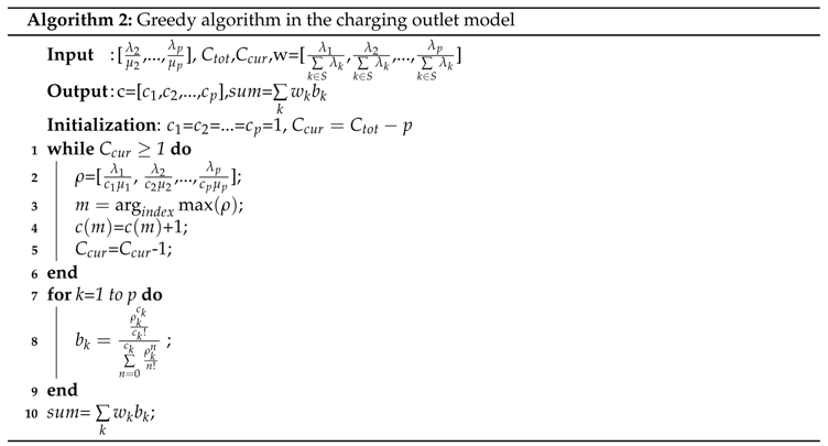
In the greedy algorithm, each FCS is allocated with one charging outlet initially. In each iteration of the whole loop, a single outlet is allocated to the FCS with the greatest value of traffic intensity. The rationale behind this is to allocate more charging outlets to the FCS with heavy loads. In each round, the traffic intensity of every FCS is updated. The next loop describes the process of calculating in FCS k, and line 10 gives the value of the objective function.
2.3. Profit Optimization Model
In this subsection, we present a profit optimization model that considers battery degradation costs and the charging characteristics. We follow the idea of limiting SoCr of the EVs to a reasonable level from [36], and our objective is to maximize the system profit. In the profit optimization model, both the charging characteristics and the battery degradation cost are addressed. This subsection consists of three parts: charging power model, battery degradation model and profit optimization formulation, as follows.
2.3.1. Charging Power Model
In direct current (DC) FCS, constant current constant voltage (CCCV) charging mode is used for Li-ion batteries. In this charging regime, the battery is charged with a constant current until the voltage reaches a certain threshold value. Once the charging voltage reaches the threshold value, the charging voltage remains constant, while the charging current decreases significantly due to the internal resistance of the battery. In fast charging station applications, constant current constant voltage (CCCV) is widely employed to minimize the battery degradation and to ensure the safety of the battery. Ref. [37] shows experimental results using CCCV for fast charging station applications and the authors in [36] develop charging power function shown in Figure 2. It is noteworthy that the charging power approximately remains constant before a threshold of energy decreases as the stored energy gets closer to maximum capacity. It is noteworthy that a similar phenomenon can be observed in daily life when charging electronic devices with Li-ion batteries. For instance, while charging cell phone batteries (Li-ion), the charging power decreases as the battery SoC reaches and charging duration gets considerable longer. Mathematically, the charging power function [36] is expressed as:
where and are the constant parameters for the decreasing power. The detailed charging power function is shown in Figure 2.
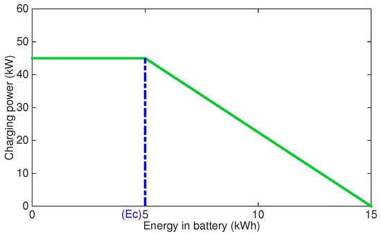
Figure 2.
Charging power function [36].
The charging duration is related to the charging power, the initial energy of the battery and the requested energy of the battery and can be expressed as:
As a result, the mean charging time and the mean charging power can be obtained from the charging time distribution, which are and , respectively. Here, is the mean value of the initial energy, as it is assumed that the initial SoC (SoCi) has a normal distribution. It is noteworthy that, by limiting SoCr, e.g., 85–90%, the mean charging time shortens compared to the full SoCr.
2.3.2. Battery Degradation Model
Electric vehicle batteries represent a large portion of the total cost. Each battery has a specific lifetime that is determined by the charging power and the charge–discharge cycles. Each time a battery is charged at a FCS, a certain amount of battery degrades, which is related to the charging duration and the charging power [38]. The expected battery degradation cost in the charging duration at FCS k is expressed as:
where parameters a, b, and c are related to the Li-ion battery, which is the most common type—degradation. The values of a, b and c can be obtained once the battery type is known. The work in [38] provides the detailed information about the battery degradation cost and the parameter description.
2.3.3. Profit Optimization Formulation
Every FCS independently regulates its value of . After completing the charging service, a customer in FCS k gains a reward . Supposedly, the reward is a linear function of , where a customer is more satisfied with the increment of . Specifically, customers charging at the same FCS gain the same reward since every customer in the same FCS accepts the same value of . The reward function is represented by:
where m and n are the constant positive parameters.
Besides the battery degradation cost, a customer has to pay an admission fee to FCS k. Therefore, the total cost for an EV at FCS k is shown as below:
A customer is ready to join the system only if the reward is greater or equal than the total cost. Hence, the largest can be obtained when , which is .
From the system operator viewpoint, the profit is a function of the arrival rate, blocking probability and the admission fee in the FCSs. Meanwhile, it encounters a penalty for blocking the EVs without serving them. Hence, the system profit of FCS k is formulated as:
The system profit is maximized by finding a set of optimal for all the FCSs of EVs. On one hand, can be gained higher with higher . On the other hand, the higher increases the blocking probability, which threatens the system performance. Hence, by deciding the optimal for every FCS k, the maximal value of the system profit can be determined. The profit optimization problem considering all FCSs is as below:
3. Numerical Evaluations
In this section, we present the results of the performed computational experiments used to evaluate the proposed model. Three case studies, namely the Arizona State highway network, the City of Raleigh, North Carolina and the North Dakota State network are considered based on the public data available for each network. The FCS and EV parameters for each cases are shown in Table 1. The values of a, b and c are adapted based on [38] for Li-ion batteries. The maximum charging power for the battery is assumed to be 45 kW and the is set to have a normal distribution , where the mean value of is 30% with 15% for the standard deviation, and it is truncated to target a SoC within .

Table 1.
Fast charging stations (FCS) and electric vehicles(EV) input parameters.
3.1. Case Study I: Arizona State Highway Network
The first case study takes the Arizona state highway system for which the hierarchical optimization framework is applied to maximize the number of vehicles that can be served with limited grid resources. As a baseline scenario, the performance of the proposed model is compared with the case when the charging outlets are allocated equally, and the case when the SoCr is not limited (SoCr = 99%) in the profit optimization model.
In Figure 3, the 25-node network of Arizona state highways, which is also used in [18], is shown and the basemap is from [39]. The links among the nodes represent the major state and interstate highways. The numbers on the links are the approximate shortest path distance with the unit mile. The size of the nodes reflects the amount of the population of the 25 cities. Moreover, the amount of each traffic flow is generated using the gravity spatial interaction model as described in Section 3, and the external flows are excluded in this case study.
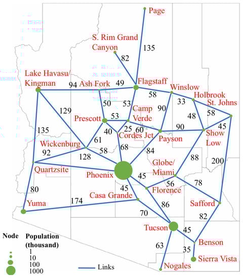
Figure 3.
Arizona highway network [18,39].
In the DC FCS, based on the parameters in Table 1, the service rate is calculated to be = 1.1 (EVs/h) when the SoCr is not limited. Moreover, it is assumed that the total number of chargers = 50. Each layer in the system is evaluated as below.
3.1.1. FCLM
To illustrate how FCLM is applied, we assume that the number of FCS locations . Solving the optimization problem presented in Section 2.1 yields location of the stations of Phoenix and Tucson to maximize the captured flow, which represents 97.29% of the whole traffic flows. Varying the number of FCS locations from 1 to 6, the captured traffic percentages are shown in the second column of Table 2.
Table 2.
Optimal charging outlet allocations.
3.1.2. Charging Outlet Allocation
The proposed greedy algorithm is applied to the charging outlet allocation, where the performance is compared with the case in which the method of equal resource allocation is used. Suppose , in equal allocation, the number of charging outlet in {Phoenix, Tucson} is {25, 25} with total weighted blocking probability 0.16. While, in the proposed method, the number of charging outlets in {Phoenix, Tucson} is {33, 17} with a total weighted blocking probability of 0.087.
The sum of the weighted blocking rate in the proposed method is 8.7%, which is lower than the case when the charging outlets are allocated equally to FCSs. We vary the number of locations for FCSs from 1 to 6, and the optimal charging outlet allocation results are shown in the third column of Table 2. Since the amount of the traffic flows going through Phoenix is dominant in the network, over half of the charging outlets are allocated to Phoenix.
3.1.3. Profit Optimization Model
Applying the optimal charging outlet allocation, the proposed method is compared to the case when is not limited, which serves as a baseline scenario. Classical FCLM was used to capture the traffic flow in the work [21], which was corresponding to the case without limiting SoCr. Hence, the proposed method of optimally limiting SoCr is compared with the case without limiting SoCr.
Four FCSs are selected as an example and the number of charging outlets remains the same, = 50. The results are shown in case I of Table 3. With the method of limiting SoCr, the system in every FCS location improves the performance compared with the case without limiting SoCr. For example, in Phoenix, the profit increases to 220.93 ($/h) and the blocking probability decreases to zero when the SoCr is limited to 95%. The average charging power increases to 16 (kW), resulting in relatively faster charging batteries compared to the case without limiting SoCr.
Table 3.
Results of profit models for three cases.
3.2. Case Study II: Raleigh City Network
In the case study of Raleigh, the performance of the proposed model is evaluated and compared with the current installed FCSs in the real world. This case study is based on the real traffic data collected from North Carolina Department of Transportation (NCDOT) in 2015 [40]. The annual average daily traffic (AADT) count of every big road is used as the input data. The network of Raleigh is shown in Figure 4, which includes 14 locations with the heaviest traffic and six current FCS locations. The base map of Figure 4 is from [41]. The current FCS locations are marked in yellow color. Numbers 1 to 6 represent the current FCS locations in Glenwood Ave, Corporate center Drive, North Carolina State University, Arrow Drive, Six forks Road and N new hope Road respectively. The shortest path in an OD pair q is used and 190 paths are placed.
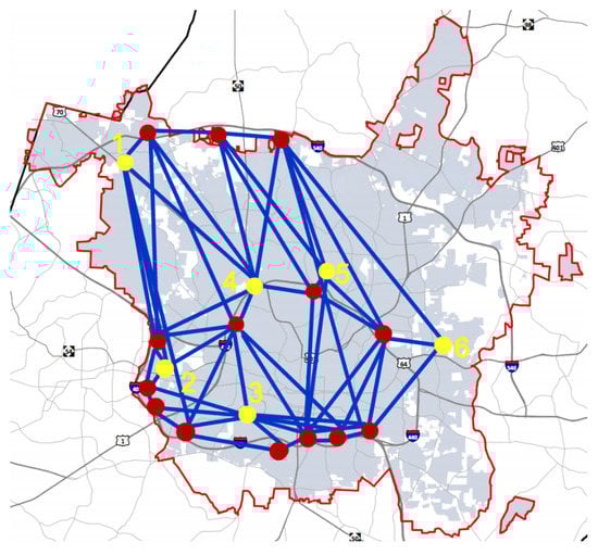
Figure 4.
The network of Raleigh city [41].
3.2.1. The Calculation of the Amount of EV Traffic Data
Using Equation (6) for the gravity spatial interaction model, the amount of traffic along the paths can be calculated. Therefore, the first step is to get the amount of traffic in the locations as the input data. It is assumed that 30% of drivers charge their EVs at CSs. From the annual average daily traffic (AADT) counts, the EV penetration rate (0.3%) in North Carolina [42], and the percentage of EV drivers charging their vehicles, the amount of traffic in the locations can be calculated. Then, the amount of traffic along the paths can be known based on the gravity spatial interaction model.
In the current FCS, the station parameters are listed in Table 4. This work assumes the service rate of EVs is 1.1, which is the case when the SoCr is at the full state. The numbers of charging outlets in these FCSs are , and 2, respectively, which taken from data in [43].
Table 4.
Current FCS parameters.
3.2.2. Comparison of Three Cases and Evaluations
There are three cases for the performance comparison, as shown below:
- Base case (BC): the case in the current station location with currently allocated chargers, which is served as a base case for the performance analysis.
- LimitSoCr (LS): the case that the proposed method of limiting SoCr is applied to the current location with currently allocated chargers.
- ReallocateChargersLimitSoCr (RCLS): the case that the number of chargers in the stations is re-allocated with limiting the SoCr is proposed.
The numerical results are shown in Figure 5 and Figure 6 are the summary of the total weighted blocking probability and the total profit for the three cases. For the case of RCLS, the optimal number of chargers are and, 1, respectively. Since the traffic intensity of FCS5 is very high in BC, resulting in the high blocking rate. From the results of our model, after relocating the charging outlets in RCLS, the blocking rate in FCS5 decreases over 1/4. In Figure 6, the system performance of RCLS is the best among three cases. The profit in the RCLS case doubles and the total weighted blocking rate decreases more than 1/3 compared to BC.
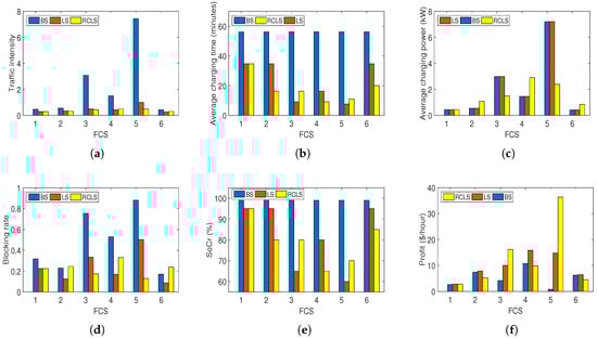
Figure 5.
Performance comparison in three cases. (a) traffic intensity; (b) average charging time (minutes); (c) average charging power (kW); (d) blocking probability; (e) SoCr (%); (f) system profit ($/h).
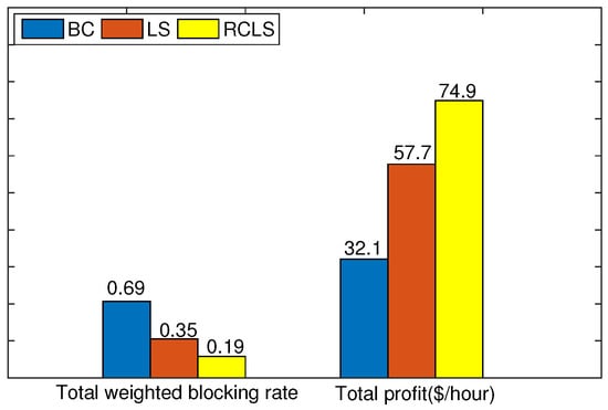
Figure 6.
Summary of performance comparison.
3.2.3. Re-Allocation of the FCSs in Raleigh Network
As more and more EVs are deployed on the road and more charger outlets are installed, the locations of FCSs and the amount of captured traffic flows become crucial to the transportation and city planning. Therefore, the case in which the FCSs and outlets are re-located in Raleigh is studied with the intention of analyzing potential future improvements. The case in which the newly added charging outlets are installed in the current FCSs, according to the proportion of the arrival rate, serves as a baseline scenario. In both cases, the method of limiting SoCr is applied.The baseline scenario is named LS while the proposed method is called RelocateLocationLimitSoCr (RLLS) for simplification.
In RLLS, the locations of re-located FCSs are shown in Figure 7 marked as green triangles. Numbers 1 to 6 represent the relocated FCS locations in Soccer park drive, Zuma way, North Carolina State University, Six forks Road, Walker street and Horton street respectively. The number of EVs that will charge in the re-located FCSs are 5.51, 2.23, 2.71, 8.06, 5.48 and 3.88, respectively, the total of which is about 1.5 times more than in the current FCSs. We assume that the total number of charging outlets increases to 20, while the other parameters remain the same.
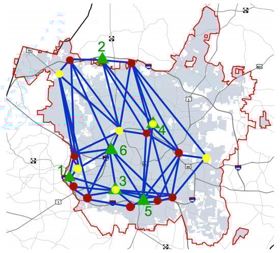
Figure 7.
Locations of fast charging station (FCS) comparison [41].
After implementing the two scenarios, the number of charging outlets in the current FCSs are: and 3, and in the re-allocated FCSs, they are , and 3, respectively. The system performance comparison is shown in Figure 8. In order to evaluate the whole network, the total weighted blocking probability and the total profit are shown in Figure 8a. In Figure 8b, the total weighted blocking probability in LS is relatively low due to the relatively low traffic intensity. However, in the RLLS case, it can capture more traffic while still keeping the gap within 5% compared to LS. From the aspect of the system profit, the profit in RLLS increases to be 163 ($/h), which increases almost 50% compared to LS.
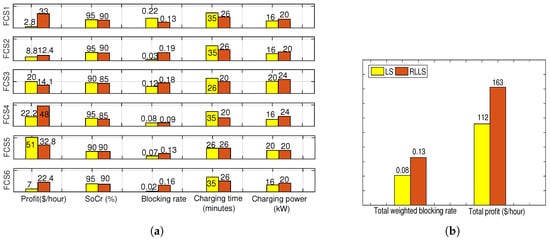
Figure 8.
Performance comparison between LimitSoCr (LS) and RelocateLocationLimitSoCr (RLLS). (a) performance in six FCSs; (b) profit and total weighted blocking rate evaluation.
In order to better illustrate the performance of the proposed method, we provide a comparison with a related work published in Ref. [21]. The re-allocated FCSs with an optimal number of charging outlets is compared with the method of FCLM reported in [21]. The results are shown in case II of Table 3. In the case with limiting SoCr, the total profit in the system is 163 ($/h), while it is 120 ($/h) in the case without limiting SoCr. By limiting SoCr, the average charging time can be shortened exponentially, which decreases the customers’ blocking probability and increases the system profit.
3.3. Case Study III: North Dakota State Network
In the third case study, the proposed model is applied to the North Dakota state network for the performance evaluation. To the best of our knowledge, there are no public FCSs in North Dakota [43]. Therefore, the case study presented in this section will shed light on the future FCS deployments. The case without limiting SoCr is served as a baseline scenario for the performance comparison.
In Figure 9, we present the North Dakota State highway network and pin the locations of the top 15 cities with highest population as the potential candidates for the FCS locations [44]. The basemap of Figure 9 is from [45]. The shortest paths between the OD pairs are used for the traffic links and a total of 105 paths are shown in the map. In Equation (6), the gravity spatial interaction model according to the node population can be used to calculate the amount of traffic along each path. Notice that EV traffic along each path can be calculated by using the amount of traffic, EV penetration rate (0.15 per a thousand people) [46], and the percentage of EV drivers charging their vehicles (30% as assumed in case II).
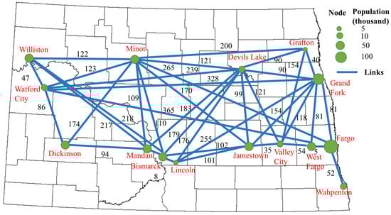
Figure 9.
The North Dakota State network [45].
First, FCLM is applied to locate FCSs, and the optimization problem is solved according to the procedure presented in Section 2.1. By varying the number of FCSs from 1 to 5, the locations and the percentage of captured traffic are shown in Table 5. When there is only one FCS to be located, the city of Fargo is selected to place an FCS with 72.91% of captured traffic. To capture over 99% of traffic, at least four FCS locations are needed.
Table 5.
Optimal FCS locations.
Next, four FCS locations with 15 charging outlets are selected as an example to evaluate the performance of the proposed model. The arrival rates of four FCS locations (Fargo, Bismarck, Grand Fork and Minot) are 16.84, 5.64, 0.54, and 0.33 EVs/h, respectively. Solving the optimal charging outlet problem presented in Section 2.2 yields 9, 4, 1 and 1 for each location. Compared to the small arrival rate of Grand Fork and Minot, Fargo is able to capture a large amount of traffic. Therefore, more than half of the charging outlets are allocated to the FCS in Fargo.
After optimizing the charging outlet allocation, the performance of the system profit model is analyzed. The case without limiting SoCr serves as a baseline for the comparison with our proposed model. In the case when customers’ SoCr is close to hundred percent, the blocking rates of all four FCSs are high, resulting in the high total weighted blocking rate and relatively low system profit. On the contrary, the total system profit of the case with limiting SoCr is 141 ($/hour), which is 1.5 times more than the profit of the case without limiting SoCr. The performance comparison is presented in Case III of Table 3. It is noteworthy that the performance of Grand Fork and Minot does not improve significantly by limiting SoCr. The rationale behind this is that the arrival rates of the two FCSs are relatively low.
3.4. Numerical Results Analysis
From the numerical results of cases I, II, and III, it is observed that the percentage of captured EVs increases when the optimal placement of CSs is applied in a network. Due to the fact that the spatial distribution of EVs is uneven, the system operator is required to properly allocate the energy resource to each CS. The results in our cases show that the proposed algorithm of resource allocation is effective in decreasing the probability of blocking EVs. Furthermore, the findings from Table 3 and Figure 6 show that limiting the SoCr to a reasonable level outperforms the case of charging the battery in full. For example, applying the strategy of limiting SoCr, the total profit increases more than one third compared to the case without limiting SoCr in Figure 6. To that end, the results in Figure 8b verify that even though increasing the number of charging outlets in currently installed CSs provides a good way to improve the system performance, it becomes less effective if the value of demand is not big enough. Therefore, it shows the importance of placing CSs and allocating energy optimally.
4. Conclusions
In this paper, we have proposed a hierarchical system model of a network of fast charging stations (FCSs) from the viewpoints of both traffic and service network. The three-layered system model is composed of the placement of FCSs, the charging outlet allocation, and the system profit model with the consideration of the Li-ion battery model. The Arizona state highway network, the Raleigh city network and the North Dakota state network are applied to evaluate the system performance of the proposed model.
The numerical results indicate that the percentage of captured electric vehicles (EVs) increases with the application of optimal CS placement. The results also demonstrate the effectiveness of the proposed resource allocation and charging strategies. The number of served EVs and the total profit of the system operator increase in the proposed model. As the charging demand is increasing rapidly, the results verify the necessity to place CSs and allocate the energy resource optimally, with the consideration of the battery charging dynamics. The proposed model can be applied to a charging stations (CSs) planning problem, assisting city planners in making decisions efficiently.
There are two promising directions of future research. The first one involves the implementation of energy storage devices in the CSs and the stochastic renewable energy scheduling problem. An energy storage device is capable of storing the energy for use when the power demand is high. Another direction of future research is considering the EV routing problem in the network with the aim of resolving the uneven demand at the CSs.
Author Contributions
Cuiyu Kong, Raka Jovanovic, Islam Safak Bayram and Michael Devetsikiotis proposed the main idea. Cuiyu Kong performed the numerical evaluation in case studies. Raka Jovanovic proposed the algorithm in the optimization model. Islam Safak Bayram, Michael Devetsikiotis, Cuiyu Kong and Raka Jovanovic designed the system models and wrote this paper.
Conflicts of Interest
The authors declare no conflict of interest.
Nomenclature
| E | The total energy in a full-charged battery |
| The threshold energy | |
| A constant parameter related to the efficiency of a system | |
| The arrival rate of customers at FCS k | |
| The expected charging power of an EV in FCS k | |
| Customer blocking probability in FCS k | |
| The number of charger outlets allocated to FCS k | |
| The fixed infrastructure cost | |
| The total number of charging outlets | |
| The penalty of k for not severing the customers | |
| A shortest path distance in a path q | |
| Initial energy of an EV | |
| Requested energy of an EV | |
| The amount of traffic on the path between OD pair q | |
| Reward of an EV customer after completing the service at FCS k | |
| K | Set of all potential FCS locations |
| Set of selected FCSs in a path q | |
| Set of potential locations in K on the path of the OD pair q | |
| p | The number of FCSs to be located |
| Maximum charging power for an EV | |
| Q | Set of all of the OD pairs |
| q | Aparticular OD pair |
| System profit of FCS k | |
| S | The set of selected FCS locations, |
| Initial SoC of an EV | |
| Requested SoC of an EV | |
| Admission fee of an EV at FCS k | |
| The weighted value in FCS k | |
| A binary decision variable, where = 1 if a FCS is allocated at k, else = 0 | |
| A binary decision variable, where = 1 if is captured, else = 0 | |
| z | A proportionality constant parameter |
| FCLM | Flow-capturing location-allocation model |
References
- United States Environmental Protection Agency. Greenhouse Gas Emissions. Available online: https://www.epa.gov/ghgemissions/sources-greenhouse-gas-emissions (accessed on 4 January 2017).
- International Energy Agency. Global EV Outlook 2016. Available online: https://www.iea.org/publications/freepublications/publication/Global_EV_Outlook_2016.pdf (accessed on 4 January 2017).
- Singer, M. Consumer Views on Plug-in Electric Vehicles—National Benchmark Report, 2nd ed.; National Renewable Energy Laboratory: Golden, CO, USA, 2016.
- Electric Vehicle Initiative. Available online: http://www.iea.org/media/topics/transport/EVI_Government_Fleet_Declaration.pdf (accessed on 4 January 2017).
- Opplysningsrådet for Veitrafikken. Available online: http://www.ofvas.no/ (accessed on 4 January 2017).
- The Statistics Portal. Breakdown of Publicly Available Electric Vehicle Chargers (EVSE) in 2015. Available online: https://www.statista.com/statistics/571564/publicly-available-electric-vehicle-chargers-by-country-type/ (accessed on 4 January 2017).
- Brenna, M.; Foiadelli, F.; Longo, M.; Zaninelli, D. e-Mobility forecast for the transnational e-corridor planning. IEEE Trans. Intell. Transp. Syst. 2016, 17, 680–689. [Google Scholar] [CrossRef]
- Hiwatari, R.; Ikeya, T.; Okano, K. A road traffic simulator to analyze layout and effectiveness of rapid charging infrastructure for electric vehicle. In Proceedings of the 2011 IEEE Vehicle Power and Propulsion Conference (VPPC), Chicago, IL, USA, 6–9 September 2011; pp. 1–6. [Google Scholar]
- Xu, F.; Yu, G.Q.; Gu, L.F.; Zhang, H. Tentative analysis of layout of electrical vehicle charging stations. East China Electr. Power 2009, 37, 1678–1682. [Google Scholar]
- Chokkalingam, B.; Padmanaban, S.; Siano, P.; Krishnamoorthy, R.; Selvaraj, R. Real-Time Forecasting of EV Charging Station Scheduling for Smart Energy Systems. Energies 2017, 10, 377. [Google Scholar] [CrossRef]
- Yan, J.; Zheng, H.; Lu, N. Temperature-load sensitivity study for adjusting MISO day-ahead load forecast. In Proceedings of the 2016 IEEE Power and Energy Society General Meeting (PESGM), Boston, MA, USA, 17–21 July 2016; pp. 1–5. [Google Scholar]
- Owen, S.H.; Daskin, M.S. Strategic facility location: A review. Eur. J. Oper. Res. 1998, 111, 423–447. [Google Scholar] [CrossRef]
- Zhang, L.; Shaffer, B.; Brown, T.; Samuelsen, G.S. The optimization of DC fast charging deployment in California. Appl. Energy 2015, 157, 111–122. [Google Scholar] [CrossRef]
- Melo, M.T.; Nickel, S.; Saldanha-Da-Gama, F. Facility location and supply chain management—A review. Eur. J. Oper. Res. 2009, 196, 401–412. [Google Scholar] [CrossRef]
- Chen, T.D.; Kockelman, K.M.; Khan, M. The electric vehicle charging station location problem: A parking-based assignment method for Seattle. In Proceedings of the 92nd Annual Meeting of the Transportation Research Board, Washington, DC, USA, 13–17 January 2013; Volume 340, pp. 13–1254. [Google Scholar]
- Lam, A.Y.; Leung, Y.W.; Chu, X. Electric vehicle charging station placement: Formulation, complexity, and solutions. IEEE Trans. Smart Grid 2014, 5, 2846–2856. [Google Scholar] [CrossRef]
- Hodgson, M.J. A Flow-Capturing Location-Allocation Model. Geogr. Anal. 1990, 22, 270–279. [Google Scholar] [CrossRef]
- Upchurch, C.; Kuby, M.; Lim, S. A Model for Location of Capacitated Alternative-Fuel Stations. Geogr. Anal. 2009, 41, 85–106. [Google Scholar] [CrossRef]
- Kuby, M.; Lim, S. The flow-refueling location problem for alternative-fuel vehicles. Socio-Econ. Plan. Sci. 2005, 39, 125–145. [Google Scholar] [CrossRef]
- Capar, I.; Kuby, M. An efficient formulation of the flow refueling location model for alternative-fuel stations. IIE Trans. 2012, 44, 622–636. [Google Scholar] [CrossRef]
- Cruz-Zambrano, M.; Corchero, C.; Igualada-Gonzalez, L.; Bernardo, V. Optimal location of fast charging stations in Barcelona: A flow-capturing approach. In Proceedings of the 2013 10th IEEE International Conference on the European Energy Market (EEM), Stockholm, Sweden, 27–31 May 2013; pp. 1–6. [Google Scholar]
- Amini, M.; Islam, A. Allocation of electric vehicles’ parking lots in distribution network. In Proceedings of the 2014 IEEE PES Innovative Smart Grid Technologies Conference (ISGT), Washington, DC, USA, 19–22 February 2014; pp. 1–5. [Google Scholar]
- Neyestani, N.; Damavandi, M.Y.; Shafie-Khah, M.; Contreras, J.; Catalão, J.P. Allocation of plug-in vehicles’ parking lots in distribution systems considering network-constrained objectives. IEEE Trans. Power Syst. 2015, 30, 2643–2656. [Google Scholar] [CrossRef]
- Amini, M.H.; Moghaddam, M.P.; Karabasoglu, O. Simultaneous allocation of electric vehicles’ parking lots and distributed renewable resources in smart power distribution networks. Sustain. Cities Soc. 2017, 28, 332–342. [Google Scholar] [CrossRef]
- Xiang, Y.; Yang, W.; Liu, J.; Li, F. Multi-Objective Distribution Network Expansion Incorporating Electric Vehicle Charging Stations. Energies 2016, 9, 909. [Google Scholar] [CrossRef]
- Amini, M.; Sarwat, A.I. Optimal reliability-based placement of plug-in electric vehicles in smart distribution network. Int. J. Energy Sci. 2014, 4, 43–49. [Google Scholar] [CrossRef]
- Brenna, M.; Foiadelli, F.; Longo, M. The exploitation of vehicle-to-grid function for power quality improvement in a smart grid. IEEE Trans. Intell. Transp. Syst. 2014, 15, 2169–2177. [Google Scholar] [CrossRef]
- Bae, S.; Kwasinski, A. Spatial and temporal model of electric vehicle charging demand. IEEE Trans. Smart Grid 2012, 3, 394–403. [Google Scholar] [CrossRef]
- Liang, H.; Sharma, I.; Zhuang, W.; Bhattacharya, K. Plug-in electric vehicle charging demand estimation based on queueing network analysis. In Proceedings of the 2014 IEEE PES General Meeting Conference & Exposition, National Harbor, MD, USA, 27–31 July 2014; pp. 1–5. [Google Scholar]
- Bayram, I.S.; Tajer, A.; Abdallah, M.; Qaraqe, K. Capacity planning frameworks for electric vehicle charging stations with multiclass customers. IEEE Trans Smart Grid 2015, 6, 1934–1943. [Google Scholar] [CrossRef]
- Xiang, Y.; Liu, J.; Li, R.; Li, F.; Gu, C.; Tang, S. Economic planning of electric vehicle charging stations considering traffic constraints and load profile templates. Appl. Energy 2016, 178, 647–659. [Google Scholar] [CrossRef]
- Yang, J.; Dong, J.; Hu, L. A data-driven optimization-based approach for siting and sizing of electric taxi charging stations. Transp. Res. C Emerg. Technol. 2017, 77, 462–477. [Google Scholar] [CrossRef]
- Leou, R.C.; Hung, J.J. Optimal Charging Schedule Planning and Economic Analysis for Electric Bus Charging Stations. Energies 2017, 10, 483. [Google Scholar] [CrossRef]
- Chen, L.; Huang, X.; Chen, Z.; Jin, L. Study of a New Quick-Charging Strategy for Electric Vehicles in Highway Charging Stations. Energies 2016, 9, 744. [Google Scholar] [CrossRef]
- Simchi-Levi, D.; Berman, O. A heuristic algorithm for the traveling salesman location problem on networks. Oper. Res. 1988, 36, 478–484. [Google Scholar] [CrossRef]
- Fan, P.; Sainbayar, B.; Ren, S. Operation analysis of fast charging stations with energy demand control of electric vehicles. IEEE Trans. Smart Grid 2015, 6, 1819–1826. [Google Scholar] [CrossRef]
- Andersson, D.; Carlsson, D. Measurement of ABB’s Prototype Fast Charging Station for Electric Vehicles. Master’s Thesis, Chalmers University of Technology, Gothenburg, Sweden, 2012. [Google Scholar]
- Ma, Z.; Zou, S.; Liu, X. A distributed charging coordination for large-scale plug-in electric vehicles considering battery degradation cost. IEEE Trans. Control Syst. Technol. 2015, 23, 2044–2052. [Google Scholar] [CrossRef]
- Free US and World Maps.Com. Arizona Counties Basemap. Available online: http://www.freeusandworldmaps.com/html/US_Counties/ALtoGACounty.html (accessed on 20 April 2017).
- North Carolina Department of Transportation. Traffic Volumne. Available online: https://www.ncdot.gov/travel/statemapping/trafficvolumemaps/ (accessed on 4 January 2017).
- City of Raleigh. City Limit Map. Available online: http://www.raleighnc.gov/business/content/ITechAdmin/Articles/MapGallery.html (accessed on 20 April 2017).
- Wescott, R.F.; Jensen, J.; Egan, C. Impact of Introducing an Electric Vehicle Tax Credit on the North Carolina State Economy Available online:. Available online: http://secureenergy.org/wp-content/uploads/2016/05/NC_EV_Study_May16.pdf (accessed on 4 January 2017).
- Plugshare. Locations of Charging Stations. Available online: https://www.plugshare.com (accessed on 4 January 2017).
- United States Census Bureau. Available online: https://factfinder.census.gov/faces/tableservices/jsf/pages/productview.xhtml?src=bkmk (accessed on 20 April 2017).
- Free US and World Maps.Com. North Dakota Counties Basemap. Available online: http://www.freeusandworldmaps.com/html/US_Counties/NMtoSCCount.html (accessed on 20 April 2017).
- ENERGY.GOV. Available online: https://energy.gov/eere/vehicles/fact-936-august-1-2016-california-had-highest-concentration-plug-vehicles-relative (accessed on 20 April 2017).
© 2017 by the authors. Licensee MDPI, Basel, Switzerland. This article is an open access article distributed under the terms and conditions of the Creative Commons Attribution (CC BY) license (http://creativecommons.org/licenses/by/4.0/).