
Automatic J–A Model Parameter Tuning Algorithm for High Accuracy Inrush Current Simulation


Abstract
:1. Introduction
- (a)
- A J–A theory based transformer model is proposed to simulate the inrush current of the power transformer.
- (b)
- The impact of each J–A parameter on the inrush current is analysed. It is found that a more accurate inrush current simulation can be achieved by tuning the J–A parameters.
- (c)
- The most representative feature of the inrush current signals is extracted as the objective function for J–A parameter tuning.
- (d)
- An automatic J–A parameter tuning algorithm is proposed and verified.
2. Inrush Current Simulation Model
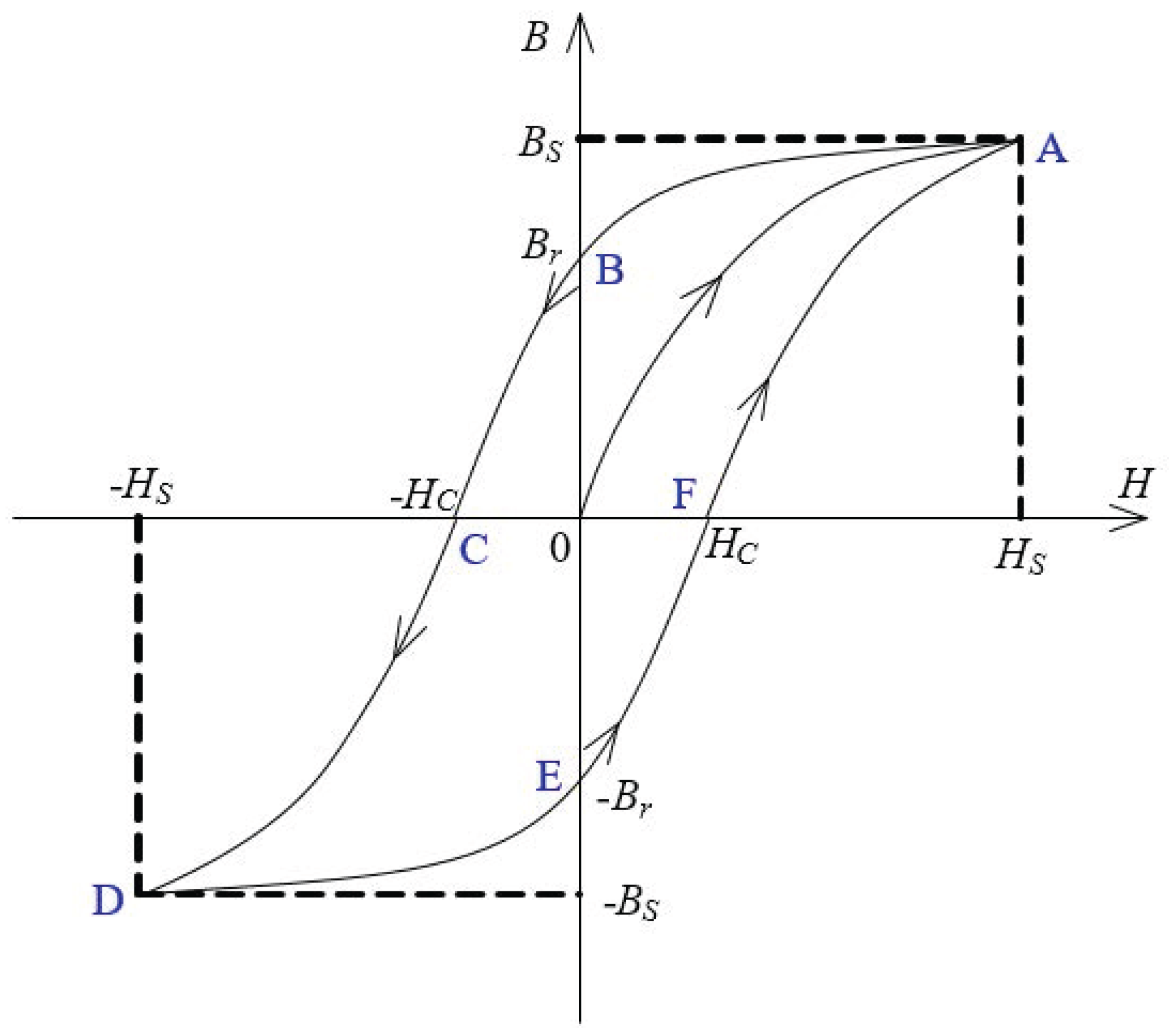
2.1. Jiles–Atherton Model
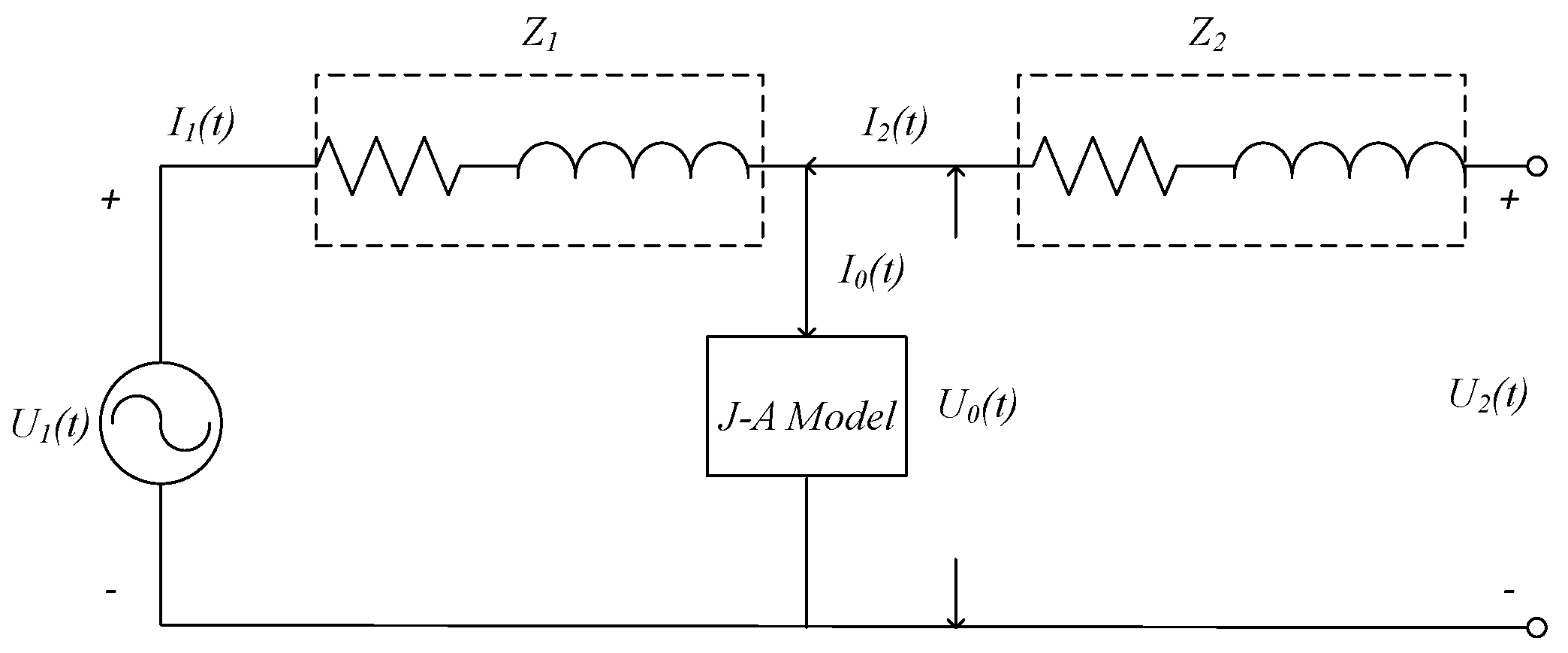
2.2. Power Transformer Simulation Model
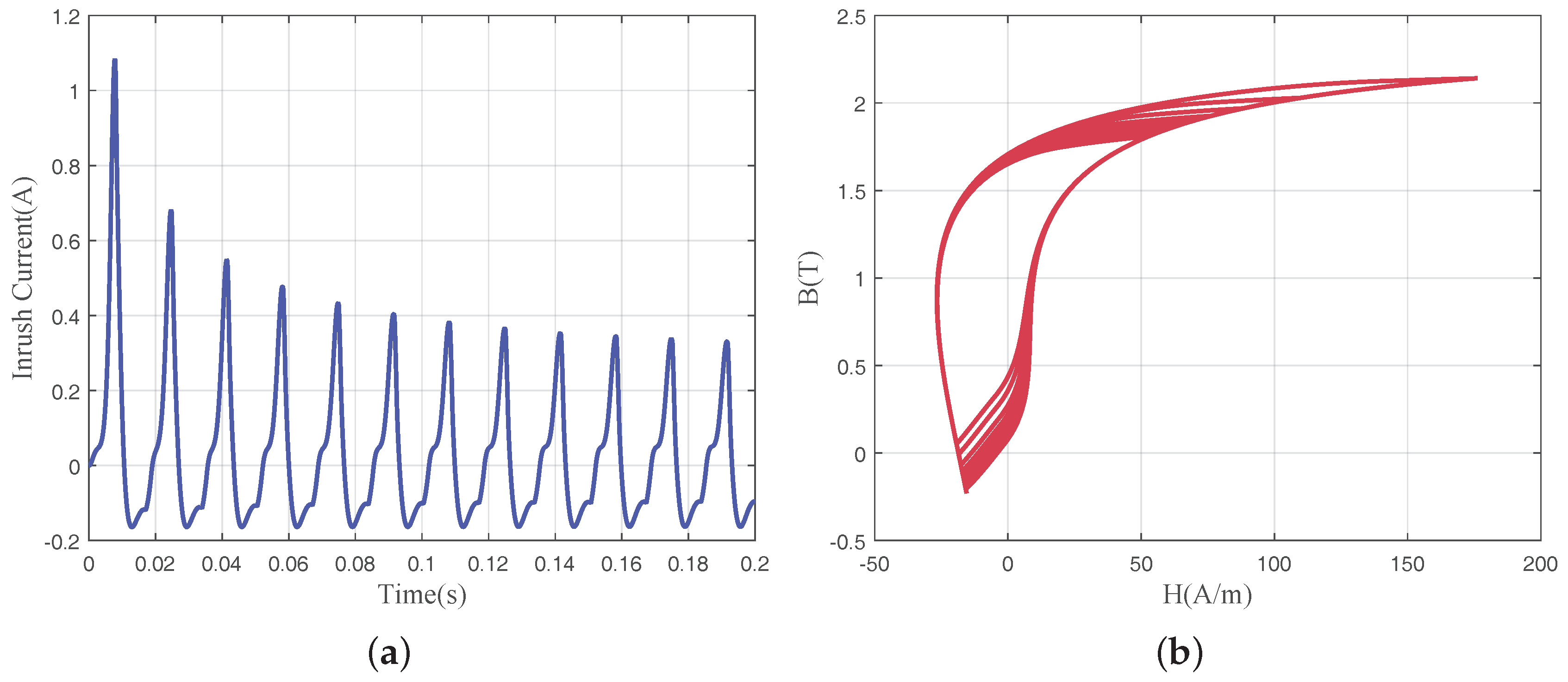
3. Inrush Current Characteristics Analysis and Key Feature Extraction
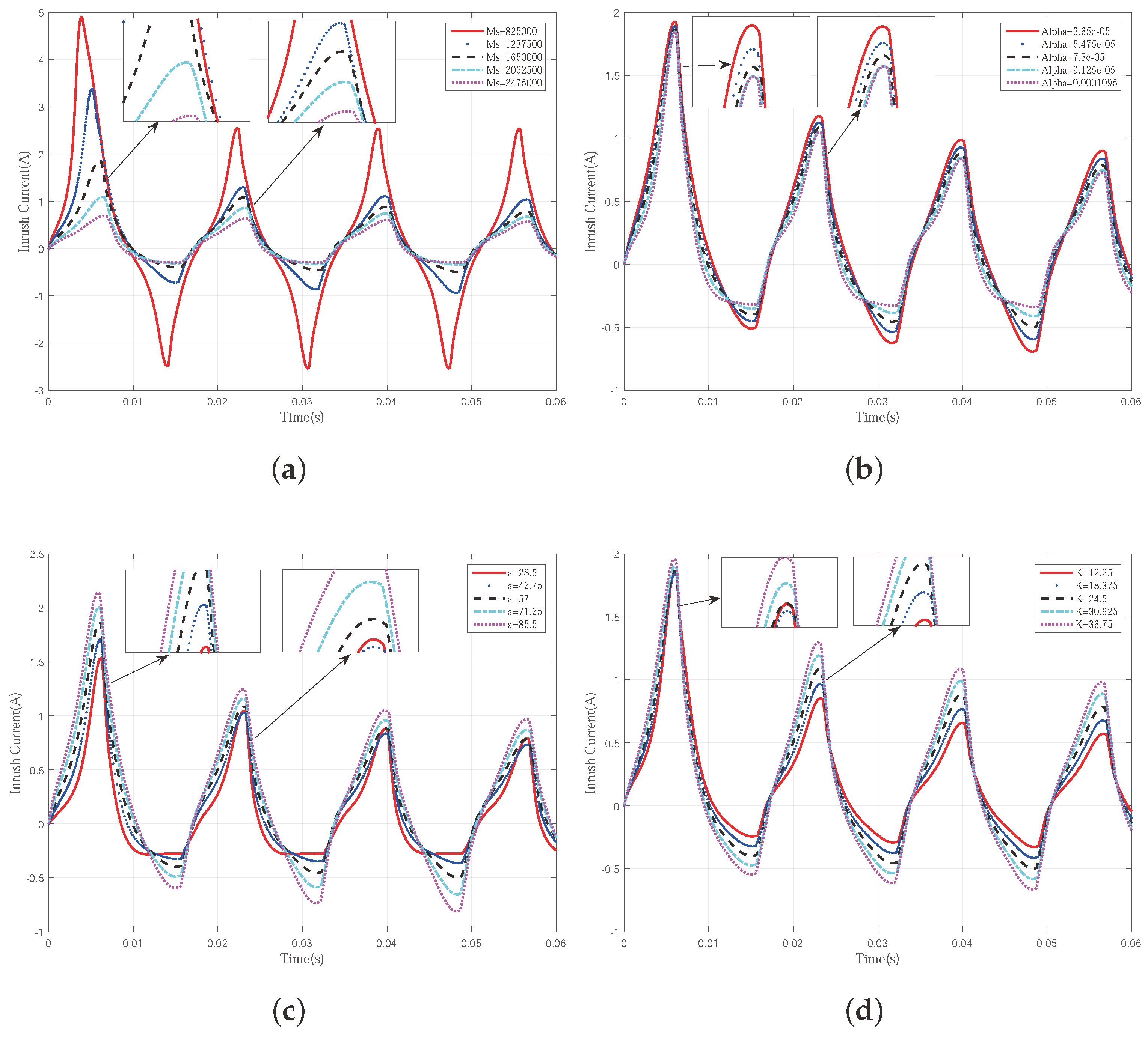
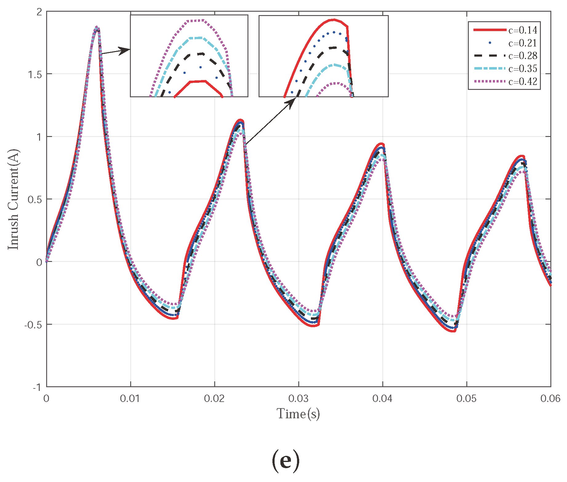
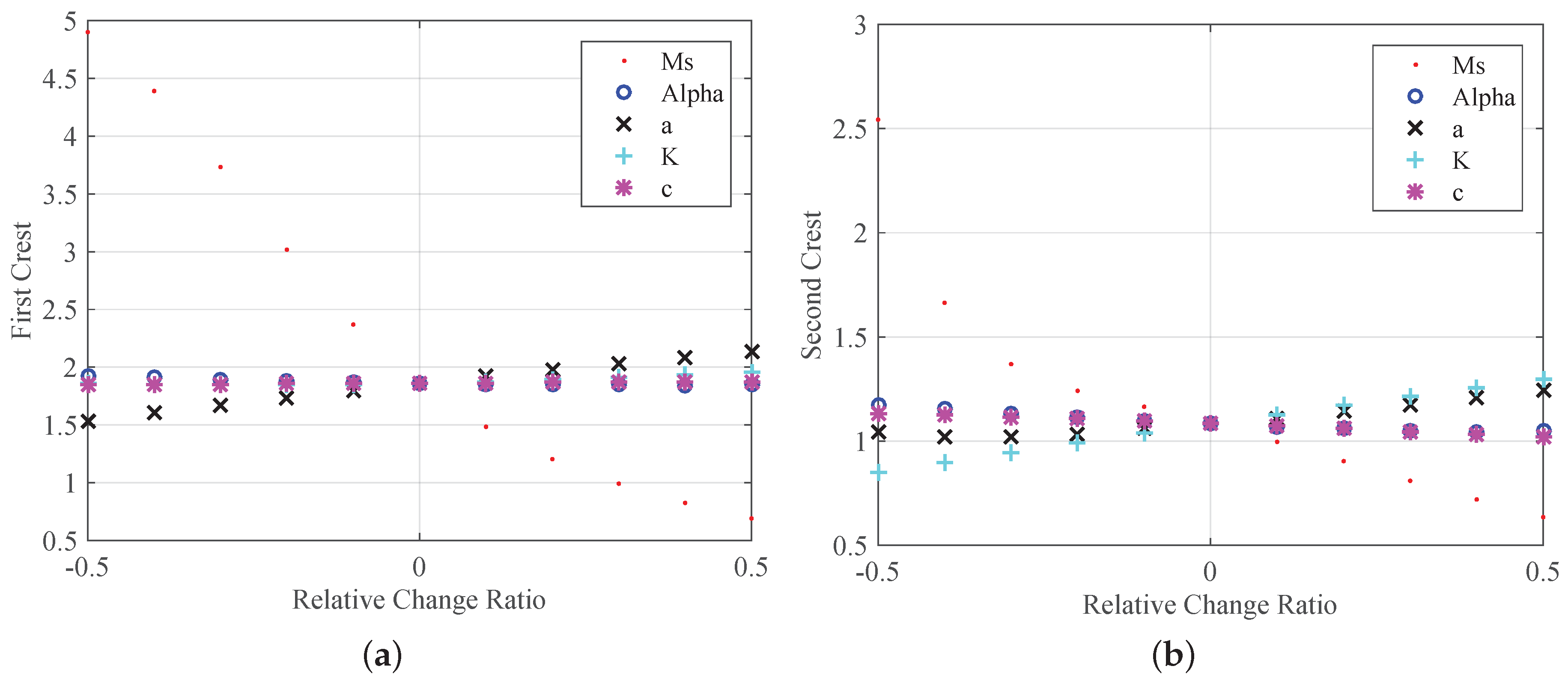
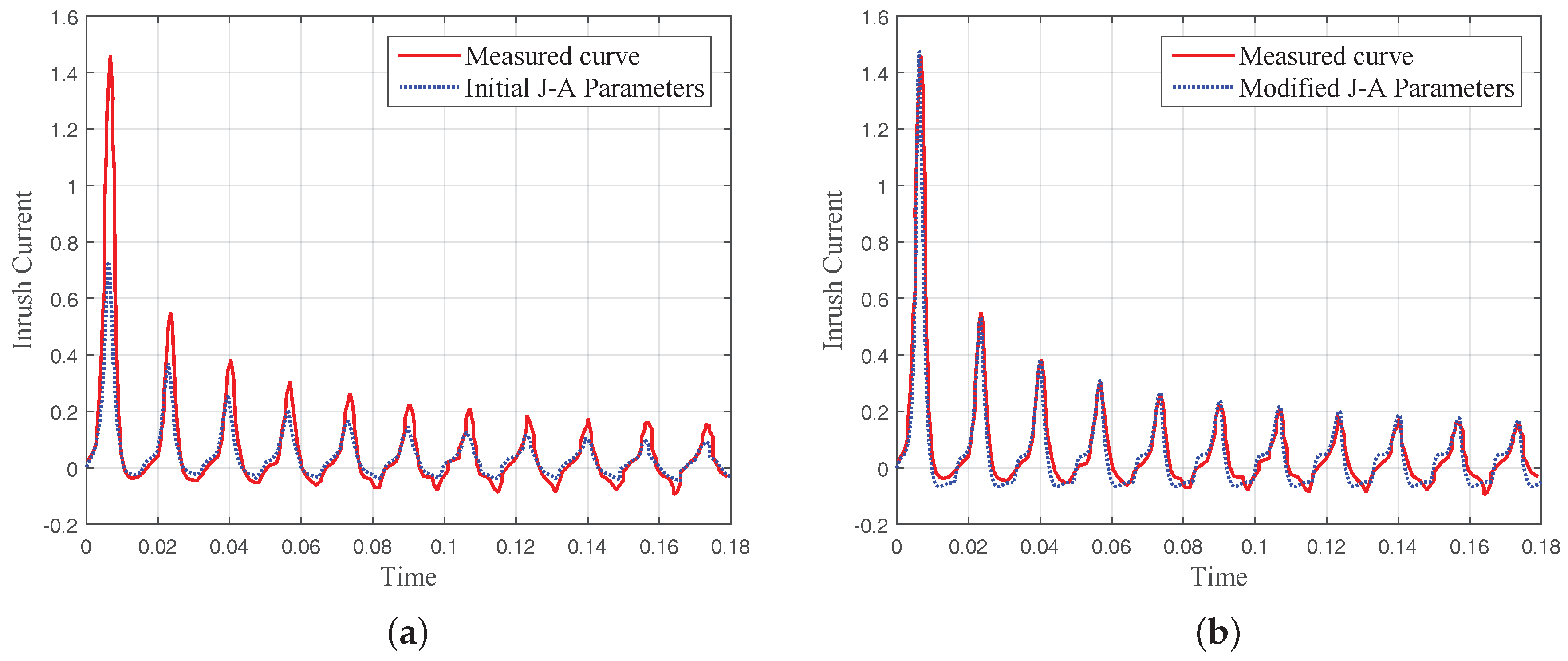
- Relativity: Different J–A parameters generate different inrush current curves. This indicates that by tuning the J–A parameters properly, the corresponding inrush current curve can be changed and thus a more accurate inrush current simulation can be achieved.
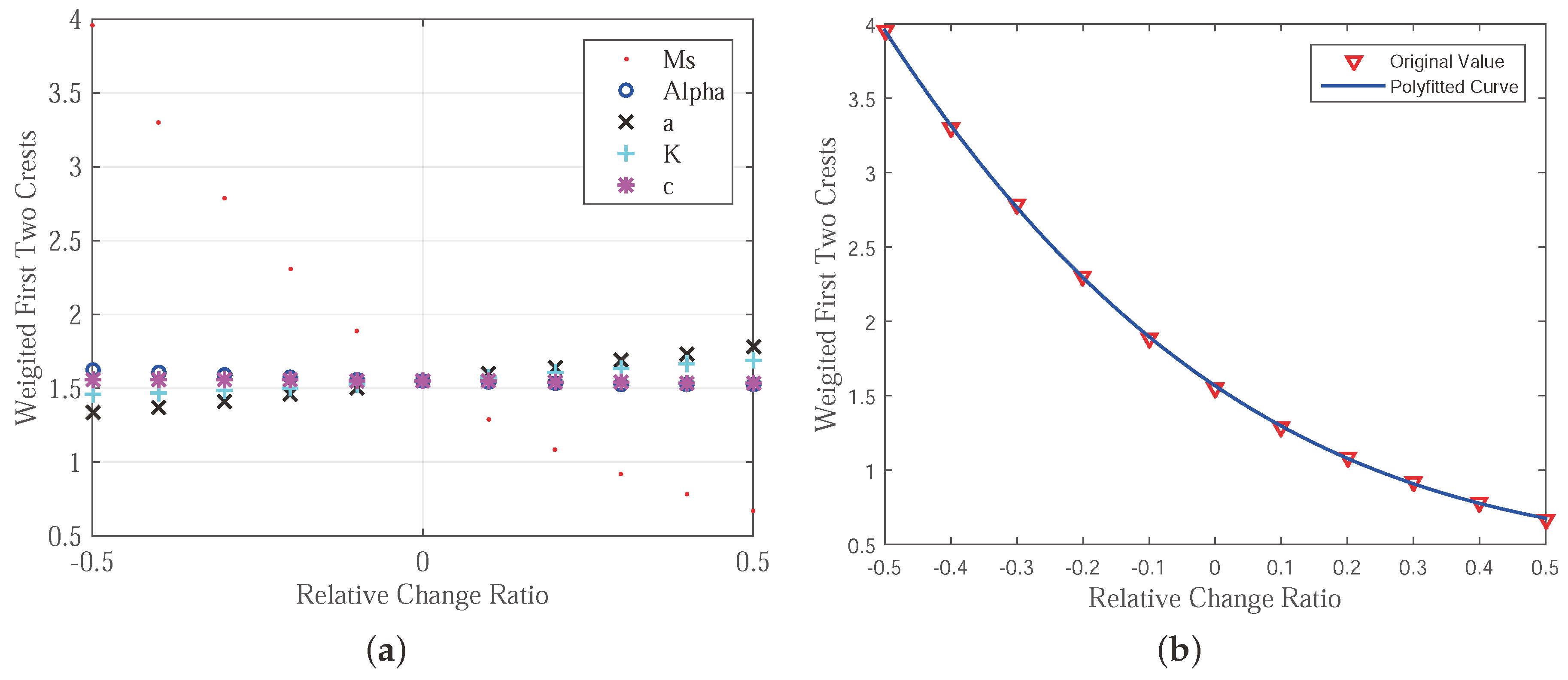
- Sensitivity: The sensitivity of the inrush current to each J–A parameter is different. As can be observed, the first period is more sensitive to the change of and a, while the second period is more sensitive to both and K. This feature indicates that, in order to improve the accuracy of the simulation efficiently, different priority shall be assigned to each of the J–A parameters. The more sensitive parameters shall be tuned first, thus the curve can approach the accurate one more quickly. Then, the small difference between the tuned curve and the true one can be compensated by tuning the less sensitive ones. The whole parameter tuning process can be accelerated significantly by separating the J–A parameters into different groups. The parameters in the primary group should be tuned firstly.
- Key Features: The inrush current curve can be featured by its first two crests. If the first two crests can be simulated precisely, the entire inrush current can be simulated precisely. From our observation, the shape and trend of the inrush current can be represented by the height of its first two crests. Two inrush current curves can be distinguished by comparing their first two crests. If the first two crests of the two curves are similar, then the two curves should also be close to each other. If the crests are far apart from each other, the following parts of the two curves should also be far away from each other. Moreover, if the first and second crests of the inrush current are significantly affected by the J–A parameters, the rest of the curves are also sensitive to the change of the J–A parameters. Furthermore, from our observation, the feature is very robust. It is very hard to find two different inrush currents with the first two crests being similar. The changing of the J–A parameters can be obviously reflected by the first two crests of the inrush current. Another reason for choosing the first two crests as a feature of the efficiency is that it is very easy to collect the data of the first two crest signals. Then, within two periods, the J–A parameters can be adjusted to more accurate values and more precise inrush current signals can be simulated.
4. Automatic Parameter Tuning Algorithm
4.1. Analysis-Based J–A Parameter Tuning
- The and a are classified as the primary parameters since they have more impact on the first and second crests of the inrush current. The rest of the parameters are classified as the secondary parameters.
- The primary parameters are tuned firstly to reduce the large difference between the simulated inrush current and the measured one. Since the curve is more sensitive to the primary parameters, the simulated one can approach the measured one quickly. In this case, both and a are reduced to increase the height of the first and second crests.
- Tuning the secondary parameters to further reduce the difference between the two curves. In this case, , K and c are all reduced. This can ensure that the simulated curve approaches the measured one and its trough does not go too deep. The small difference generated by the tuned primary parameters can be compensated by the tuned secondary parameters.
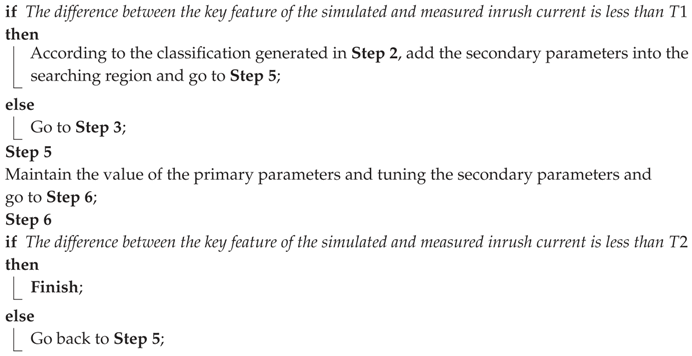
4.2. Automatic Algorithm for J–A Parameter Tuning
| Algorithm 1: Framework of the proposed algorithm. |
| Input: 1. Initial J–A parameters, 2. The Measured inrush current, 3. Threshold and |
| Output: The modified J–A parameters |
|
5. Experimental Results and Analysis
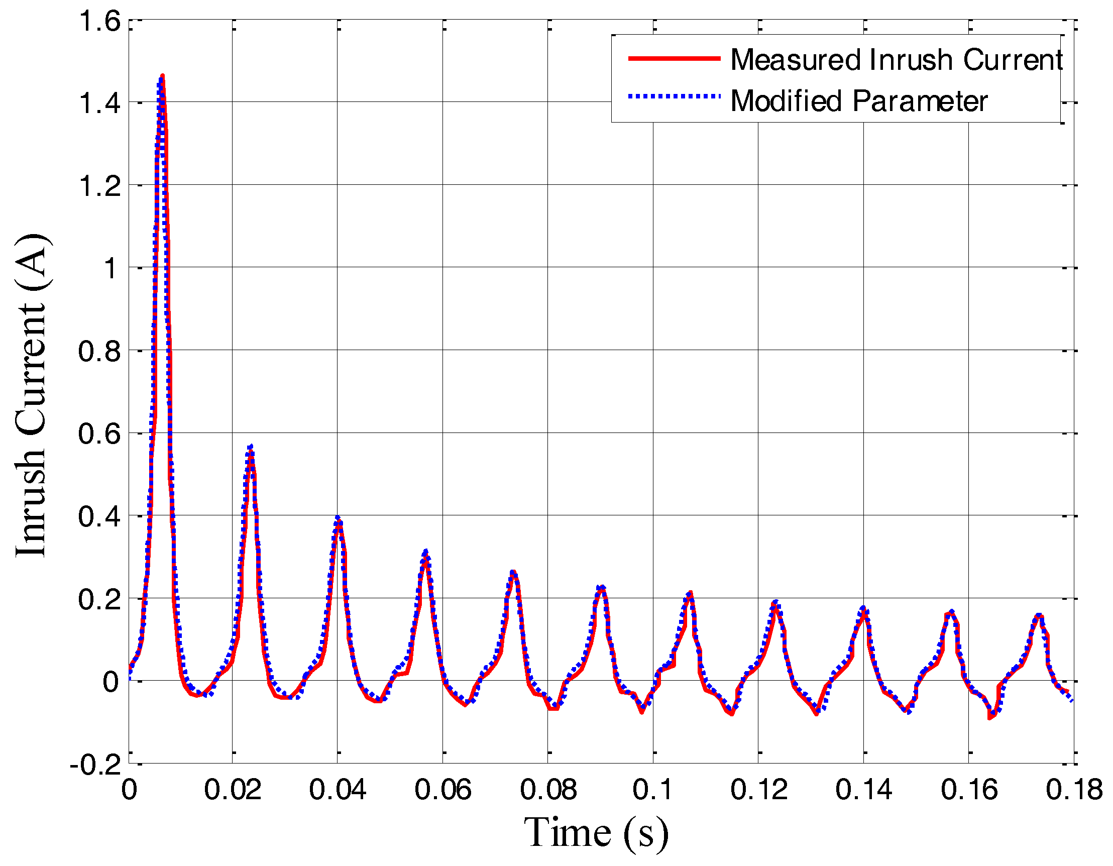
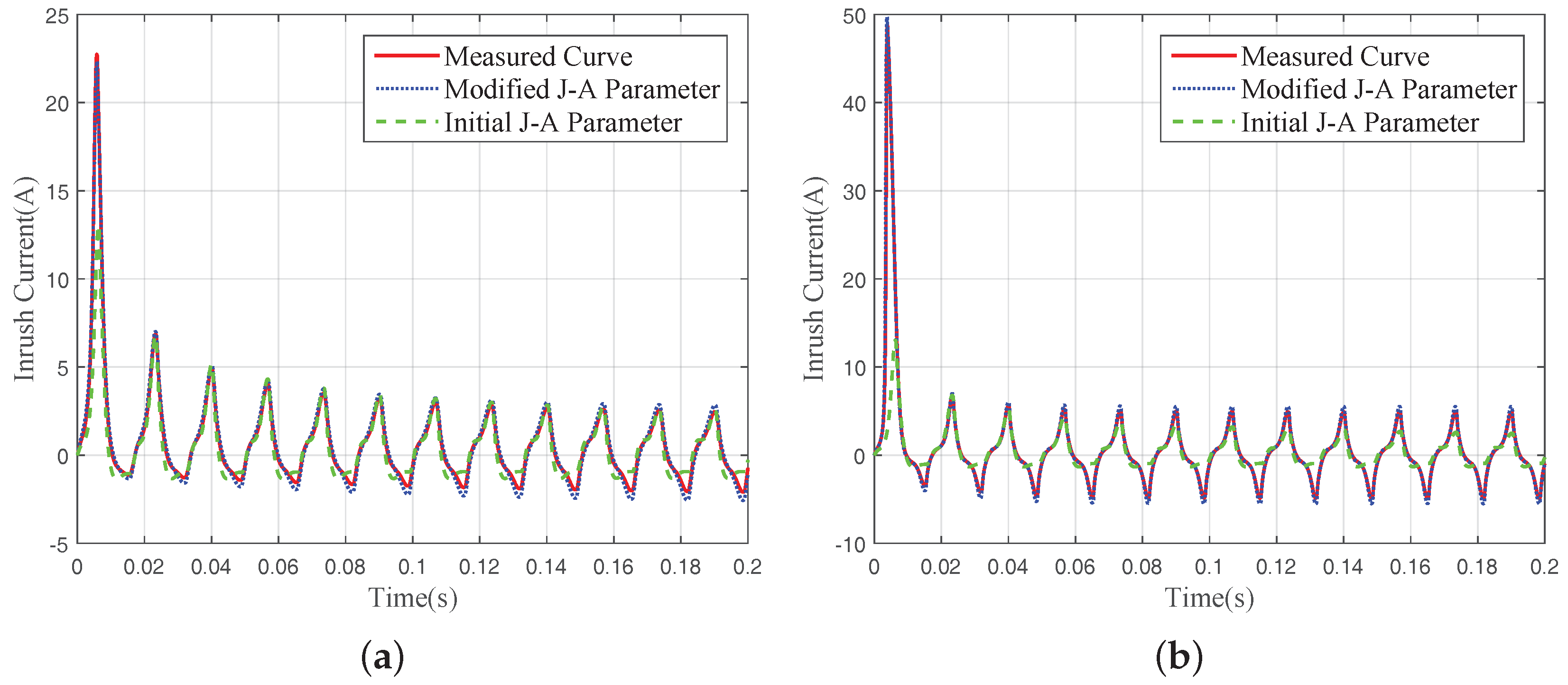
5.1. Experimental Results
5.2. Analysis and Discussion
6. Conclusions
Acknowledgments
Author Contributions
Conflicts of Interest
References
- Lin, C.E.; Cheng, C.L.; Huang, C.L.; Yeh, J.C. Investigation of magnetizing inrush current in transformers. I. Numerical simulation. IEEE Trans. Power Deliv. 1993, 8, 246–254. [Google Scholar] [CrossRef]
- Lin, C.E.; Cheng, C.L.; Huang, C.L.; Yeh, J.C. Investigation of magnetizing inrush current in transformers. II. Harmonic analysis. IEEE Trans. Power Deliv. 1993, 8, 255–263. [Google Scholar] [CrossRef]
- Ling, P.C.; Basak, A. Investigation of magnetizing inrush current in a single-phase transformer. IEEE Trans. Magn. 1988, 24, 3217–3222. [Google Scholar] [CrossRef]
- Abdulsalam, S.G.; Xu, W.; Neves, W.L.A.; Liu, X. Estimation of Transformer Saturation Characteristics from Inrush Current Waveforms. IEEE Trans. Power Deliv. 2006, 21, 170–177. [Google Scholar] [CrossRef]
- Monteiro, T.C.; Martinz, F.O.; Matakas, L.; Komatsu, W. Transformer Operation at Deep Saturation: Model and Parameter Determination. IEEE Trans. Ind. Appl. 2012, 48, 1054–1063. [Google Scholar] [CrossRef]
- Popov, M.; van der Sluis, L.; Paap, G.C.; Schavemaker, P.H. On a hysteresis model for transient analysis. Power Eng. Rev. 2000, 20, 53–55. [Google Scholar] [CrossRef]
- Jiles, D.C.; Atherton, D.L. Theory of ferromagnetic hysteresis. J. Magn. Magn. Mater. 1986, 61, 48–60. [Google Scholar] [CrossRef]
- Sima, W.; Yang, M.; Yang, Q.; Yuan, T.; Zou, M. Simulation and experiment on a flexible control method for ferroresonance. IET Gener. Transm. Distrib. 2014, 8, 1744–1753. [Google Scholar] [CrossRef]
- Ahmadi, M.; Samet, H.; Ghanbari, T. Discrimination of internal fault from magnetising inrush current in power transformers based on sine-wave least-squares curve fitting method. IET Sci. Meas. Technol. 2015, 9, 73–84. [Google Scholar] [CrossRef]
- Shah, A.M.; Bhalja, B.R. Discrimination Between Internal Faults and Other Disturbances in Transformer Using the Support Vector Machine-Based Protection Scheme. IEEE Trans. Power Deliv. 2014, 28, 1508–1515. [Google Scholar] [CrossRef]
- Ge, B.; de Almeida, A.T.; Zheng, Q.; Wang, X. An equivalent instantaneous inductance-based technique for discrimination between inrush current and internal faults in power transformers. IEEE Trans. Power Deliv. 2005, 20, 2473–2482. [Google Scholar]
- Yabe, K. Power differential method for discrimination between fault and magnetizing inrush current in transformers. IEEE Trans. Power Deliv. 1997, 12, 1109–1118. [Google Scholar] [CrossRef]
- Ashesh, M.S.; Bhavesh, R.B. Fault discrimination scheme for power transformer using random forest technique. IET Gener. Transm. Distrib. 2016, 10, 1431–1439. [Google Scholar]
- Bigdeli, M.; Vakilian, M.; Rahimpour, E. Transformer winding faults classification based on transfer function analysis by support vector machine. IET Electr. Power Appl. 2012, 6, 268–276. [Google Scholar] [CrossRef]
- Shah, A.M.; Bhalja, B.R. Discrimination between internal faults and other disturbances in transformer using the support vector machine-based protection scheme. IEEE Trans. Power Deliv. 2013, 28, 1508–1515. [Google Scholar] [CrossRef]
- Perez, L.G.; Flechsig, A.J.; Meador, J.L.; Obradovic, Z. Training an artificial neural network to discriminate between magnetizing inrush and internal faults. IEEE Trans. Power Deliv. 1994, 9, 434–441. [Google Scholar] [CrossRef]
- Zaman, M.R.; Rahman, M.A. Experimental testing of the artificial neural network based protection of power transformers. IEEE Trans. Power Deliv. 1998, 13, 510–517. [Google Scholar] [CrossRef]
- Zirka, S.E.; Moroz, Y.I.; Arturi, C.M.; Chiesa, N.; Hoidalen, H.K. Topology-correct reversible transformer model. IEEE Trans. Power Deliv. 2012, 27, 2037–2045. [Google Scholar] [CrossRef]
- Chiesa, N.; Mork, B.A.; Hidalen, H.K. Transformer model for inrush current calculations: Simulations, measurements and sensitivity analysis. IEEE Trans. Power Deliv. 2010, 25, 2599–2608. [Google Scholar] [CrossRef]
- Chiesa, N.; Hidalen, H.K. Systematic switching study of transformer inrush current: Simulation and measurements. In Proceedings of the International Conference on Power System Transients, Kyoto, Japan, 3–6 June 2009. [Google Scholar]
- Wang, X.; Thomas, D.W.P.; Sumner, M.; Paul, J.; Lopes Cabral, S.H. Characteristics of Jiles–Atherton model parameters and their application to transformer inrush current simulation. IEEE Trans. Magn. 2008, 44, 340–345. [Google Scholar] [CrossRef]
- Rudez, U.; Mihalic, R. A reconstruction of the WAMS-Detected transformer sympathetic inrush phenomenon. IEEE Trans. Smart Grid 2016, PP, 99. [Google Scholar] [CrossRef]
- Jiles, D.C.; Thoelke, J.B. Theory of ferromagnetic hysteresis: Determination of model parameters from experimental hysteresis loops. IEEE Trans. Magn. 1989, 25, 3928–3930. [Google Scholar] [CrossRef]
- Jiles, D.C.; Thoelke, J.B.; Devine, M.K. Numerical determination of hysteresis parameters for the modeling of magnetic properties using the theory of ferromagnetic hysteresis. IEEE Trans. Magn. 1992, 28, 27–35. [Google Scholar] [CrossRef]
- Lederer, D.; Igarashi, H.; Kost, A.; Honma, T. On the parameter identification and application of the Jiles–Atherton hysteresis model for numerical modelling of measured characteristics. IEEE Trans. Magn. 1999, 35, 1211–1214. [Google Scholar] [CrossRef]
- Naghizadeh, R.A.; Vahidi, B.; Hosseinian, S.H. Modelling of inrush current in transformers using inverse Jiles–Atherton hysteresis model with a Neuro-shuffled frog-leaping algorithm approach. IET Eletr. Power Appl. 2012, 6, 727–734. [Google Scholar] [CrossRef]
- Xue, D.; Chen, Y.Q. System Simulation Techniques with Matlab and Simulink; John Wiley & Sons: Hoboken, NJ, USA, 2013. [Google Scholar]
- Toman, M.; Stumberger, G.; Drago, D. Parameter identification of the Jiles–Atherton hysteresis model using differential evolution. IEEE Trans. Magn. 2008, 44, 1098–1101. [Google Scholar] [CrossRef]


| Capacity | Frequency | Rated Voltage Ratio | Turn Ratio | Phase |
|---|---|---|---|---|
| 400 VA | 60 Hz | 440 V/440 V | 727/727 | single |
| Type | c | ||||
|---|---|---|---|---|---|
| Initial J–A Parameters | 1,950,000 | 35 | 0.000073 | 10.4 | 0.391 |
| Modified J–A Parameters | 1,650,000 | 17 | 0.000037 | 4.5 | 0.28 |
| Experiment | c | ||||
|---|---|---|---|---|---|
| Set 1 | 1,733,160 | 38.5 | 0.000062 | 4.1 | 0.6256 |
| Set 2 | 1,542,670 | 40 | 0.00006 | 9.1 | 0.5 |
| Set 2 | 980,325 | 20 | 0.000055 | 7.1 | 0.3374 |
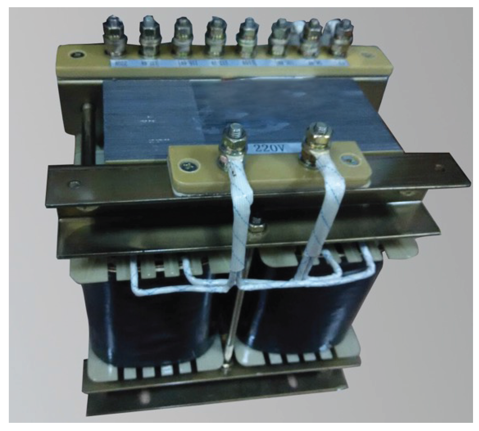
| Capacity | Frequency | Rated Voltage Ratio | Turn Ratio | Phase |
|---|---|---|---|---|
| 1000 VA | 50 Hz | 220 V/220 V | 100/100 | single |
© 2017 by the authors. Licensee MDPI, Basel, Switzerland. This article is an open access article distributed under the terms and conditions of the Creative Commons Attribution (CC BY) license (http://creativecommons.org/licenses/by/4.0/).
Share and Cite
Wen, X.; Zhang, J.; Lu, H. Automatic J–A Model Parameter Tuning Algorithm for High Accuracy Inrush Current Simulation. Energies 2017, 10, 480. https://doi.org/10.3390/en10040480
Wen X, Zhang J, Lu H. Automatic J–A Model Parameter Tuning Algorithm for High Accuracy Inrush Current Simulation. Energies. 2017; 10(4):480. https://doi.org/10.3390/en10040480
Chicago/Turabian StyleWen, Xishan, Jingzhuo Zhang, and Hailiang Lu. 2017. "Automatic J–A Model Parameter Tuning Algorithm for High Accuracy Inrush Current Simulation" Energies 10, no. 4: 480. https://doi.org/10.3390/en10040480
APA StyleWen, X., Zhang, J., & Lu, H. (2017). Automatic J–A Model Parameter Tuning Algorithm for High Accuracy Inrush Current Simulation. Energies, 10(4), 480. https://doi.org/10.3390/en10040480