
Determining the Minimal Power Capacity of Energy Storage to Accommodate Renewable Generation


State Key Laboratory of Advanced Electromagnetic Engineering and Technology, School of Electrical and Electronic Engineering, Huazhong University of Science and Technology, 1037 Luoyu Road, Wuhan 430074, Hubei, China
*
Author to whom correspondence should be addressed.
Energies 2017, 10(4), 468; https://doi.org/10.3390/en10040468
Submission received: 15 February 2017
/
Revised: 23 March 2017
/
Accepted: 24 March 2017
/
Published: 2 April 2017
(This article belongs to the Section D: Energy Storage and Application)
Abstract
:The increasing penetration of renewable generation increases the need for flexibility to accommodate for growing uncertainties. The level of flexibility is measured by the available power that can be provided by flexible resources, such as dispatachable generators, in a certain time period under the constraint of transmission capacity. In addition to conventional flexible resources, energy storage is also expected as a supplementary flexible resource for variability accommodation. To aid the cost-effective planning of energy storage in power grids with intensive renewable generation, this study proposed an approach to determine the minimal requirement of power capacity and the appropriate location for the energy storage. In the proposed approach, the variation of renewable generation is limited within uncertainty sets, then a linear model is proposed for dispatchable generators and candidate energy storage to accommodate the variation in renewable generation under the power balance and transmission network constraints. The target of the proposed approach is to minimize the total power capacity of candidate energy storage facilities when the availability of existing flexible resources is maximized. After that, the robust linear optimization method is employed to convert and solve the proposed model with uncertainties. Case studies are carried out in a modified Garver 6-bus system and the Liaoning provincial power system in China. Simulation results well demonstrate the proposed optimization can provide the optimal location of energy storage with small power capacities. The minimal power capacity of allocated energy storage obtained from the proposed approach only accounts for 1/30 of the capacity of the particular transmission line that is required for network expansion. Besides being adopted for energy storage planning, the proposed approach can also be a potential tool for identifying the sufficiency of flexibility when a priority is given to renewable generation.
1. Introduction
Integrating renewable energy is considered as a pathway to de-carbonize the power sector. The increasing penetration levels of variable renewable energy increase the need for sufficient flexible resources. Evaluation of flexibility is important to power systems with integrated intensive renewable generation [1,2].
The International Energy Agency has formally stated the concept of flexibility as an ability for balancing variability, and developed the flexibility assessment (FAST) method in [3]. In the FAST, the level of flexibility is measured by the power available for upward and downward adjustment in a given time frame. The available flexible resources considered in the FAST approach are diversified into dispatchable power plants, energy storage, interconnection between adjacent power systems and demand side management. Considering the availability, existing dispatchable power plants are the major flexible resources. The level of flexibility provided by existing power plants has a great impact on the grid integration of renewable generation. Take the northeastern region in China as an example. This vast region holds the greatest physical potential for wind energy in China. The generation mix in this region is dominated by combined heat and power (CHP) plants. The available wind power is great during the winter season. However, the flexibility provided from CHP plants is heavily limited during the winter periods because of the heat demand constraint. The relatively inflexible operational characteristics of coal-fired generators result in severe wind power curtailment [4]. The level of flexibility provided by interconnections primarily depends on the transmission capacity and long-term electricity contracts for power exchange. The long-term electricity contracts are negotiated by both sides based on the forecast of electricity demand and expected utilization hours of generators. Schedules of power exchange for the operational stage are determined by the long-term contracts and transmission capacity. The demand side management comprises various approaches to modify the behavior of end-use electricity, for example, peak shaving, valley filling, and load shifting, and provide flexibility to accommodate variable renewable generation in terms of electricity demand. A mature market and policies for the demand side management are required so that end-use consumers can be encouraged for financial incentives.
Energy storage, with the ability to deliver and absorb generation and provide energy time-shift, is regarded as a valuable tool in system operations for aiding a temporary power balance. In addition to the traditional services, such as power quality improvement [5,6], load following [7], system blackout [8], system stability [9,10] and congestion management [11], energy storage is strongly promoted to increase the level of flexibility for systems to accommodate variable generation [12]. Energy storage has been found to be efficient and beneficial in mitigating fluctuations on renewable generation [13], maintaining power balance in systems with intensive wind energy [14], and providing short-term frequency response for wind farms [15]. The need for energy storage planning is increasing [16]. Various methods quantifying the capacity of energy storage have been reported recently. In distributed grids, energy storage is an essential part of the resource portfolio and makes a great contribution to ensuring the security of local energy supply during islanding mode [17]. In transmission grids, energy storage is allowed to participate in power balance to achieve an economical operation and a maximum integration for renewable generation [18]. Basically, energy storage is characterized by energy and power capacities. A higher energy capacity allows the energy storage to respond to longer generation mismatches, while a higher power capacity allows for the quick response in a short period of time with a large magnitude [19]. Several planning models and approaches have been presented to determine the power and energy capacities of energy storage and appropriate locations according to the function of energy storage in the power system and type of technology [20,21,22].
In this paper, we present an approach to determine the minimal power capacity of energy storage from the aspect of providing flexibility to accommodate variability from high penetration levels of renewable generation. Existing dispatchable generators are considered as the primary flexible resources. Energy storage is considered as an option to increase the level of flexibility. The power capacity of energy storage represents the maximum upward and downward power that can be provided to accommodate uncertain renewable generation in a certain time interval. A linear model is proposed to describe how dispatchable generators and energy storage respond to the variability in renewable generation. Impacts of variable renewable generation on the power flow of transmission lines are also considered. Employing the proposed model, the need for energy storage is quantified. If the energy storage is required to improve the level of flexibility, the minimal power capacity and the appropriate location are then determined. From this aspect, the proposed model can be employed as a flexibility assessment tool to determine whether the level of flexibility provided by existing dispatchable generators and transmission capacity is sufficient or limited. Our approach is different from the FAST approach which assesses the level of flexibility by identifying the availability of flexible resources and offering scores. Compared with the statistic approaches conducted in FAST, our approach indicates the sufficiency of flexibility by optimizing the need for energy storage. If insufficient, the optimal allocation of energy storage, including power capacity and the location in the power grid, could be obtained and provided to decision makers. In addition, the uncertainty in renewable generation is modeled in our approach and handled by the advanced robust linear optimization.
In this study, the power-related service of the energy storage is mainly considered; thus, the energy capacity is not optimized and the discharging and charging dynamics of energy storage are not considered. Basically, given the required power capacity, the rated energy capacity can be determined according to the energy time-shift requirement represented by designed discharging time. The dynamics of energy storage, modeled by discharging and charging status and state-of-charge at each time interval, are usually incorporated into unit commitment and economic dispatch models to model the contribution of energy storage in chronological power balance. These characteristics are not the focus of this study when quantifying the need for energy storage. In addition, the generation and transmission network expansion and demand side management are not addressed when planning the energy storage.
The remainder of this paper is organized as follows. The model to determine the minimal power capacity of energy storage is presented in Section 2. The robust counterpart of the original optimization with uncertainty is presented in Section 3. Results from different cases are illustrated in Section 4 and conclusions are presented in Section 5.
2. Model
In this section, we present the model describing how dispatchable generators and energy storage accommodate the uncertainty in the renewable generation. We also show impacts of uncertain renewable generation on constraints of power balance and the transmission network.
2.1. Uncertainty Sets for Renewable Generation
The generation from wind and solar power can be highly variable. A sufficient level of flexibility is thus required to accommodate variability from renewable generation for power balance. In this study, wind farms are considered as the major types of renewable energies in a certain power system, modeled by uncertainty sets. The proposed approach is also appropriate for modeling the uncertainty in solar generation and assessing the need for energy storage in a power grid with a high penetration level of solar energy.
The polyhedral uncertainty sets are employed to model the power output from wind farms. In this uncertainty set, power output from the jth wind farm, , is restricted by the lower and upper bounds , , respectively:
The lower and upper bound values for wind power are known. The actual value for wind power is modeled as a uncertain parameter that can take any value within the interval defined in the uncertainty set (1). The uncertain parameter can be expressed as . denotes the mean value of , reflecting the average level of generation. is the deviation to the mean value for each possible realization of .
where the lower bound , and the upper bound . It is obviously observed that the mean value of is equal to 0, , and .
2.2. Accommodating the Uncertainty
The power system with a high level of flexibility can utilize existing generators to accommodate variation from renewable generation under transmission network constraints. However, if generators cannot provide sufficient flexibility to cope with the uncertainty in wind power, energy storage facilities would be taken into account as a supplementary flexible resource.
The level of flexibility in generators differs considerably. Generators with little adjustable ability, such as base-load generators operating at a set-point power, are not regarded as flexible resources. Dispatchable generators are required to adjust their output upward and downward when coping with the variability. The adjustment from the ith dispatchable generator is assumed to be linear with respect to the wind power variation.
The adjustable coefficient describes the ability that is available for the ith dispatchable generator to cope with wind power variation from the jth wind farm. is modeled as a deterministic variable to be optimized. is the number of wind farms. The negative sign in (3) indicates that if power output from the jth wind farm is above the average level, the ith generator would lower the output, and vice versa. Thus, the integration of wind power is given the priority. The operation range of ith dispatchable generator is formulated as:
where and are the lower and upper bounds of the operation range, and is the average power output from the ith dispatchable generator when the average wind power is considered. is equal to the rated capacity of the ith generator, and depends on the minimum generation level.
Similarly, the adjustment of kth energy storage with respect to can be also addressed with a linear relationship.
The adjustable coefficient denotes the ability of kth energy storage to accommodate variability from the jth wind generation, considered as a positive variable to be optimized. The magnitude of is highly depended on the realization of and the power capacity of energy storage .
Constraints (3) and (5) describe the level of flexibility provided by dispatchable generators and energy storage respectively, with respect to the realization of wind power variation. Considering the priority of wind generation, the variation of wind power requires a corresponding adjustment of the power output from generators and/or energy storage. This requirement is represented as (7).
where is the number of dispatchable generators. Derived from (7), the optimal solutions of and in the constraint (8) would determine which flexible resource is available to accommodate variable generation of the jth wind farm. Compared with the energy storage, a higher priority is given to existing flexible generators to accommodate variable renewable generation, thus the need for energy storage can be minimized.
2.3. Transmission Network Constraint
The amount and direction of power exchange through transmission lines would change when accommodating variability from renewable generation. According to the dc power flow model, the existing transmission network constraints are composed of , and . , , are vectors of power flow, bus injected power, and phase angle. is the relational matrix, is the imaginary part of the bus admittance matrix, and is the transmission capacity vector. To reduce the number of constraints and variables, we eliminate the intermediate vector as follows: (1) select a bus as the slack bus; (2) delete the slack bus’s column in and the slack bus’s row and column in to obtain sub-matrixes and ; (3) formulate the line-bus power relational matrix composed of and an all-zero-element column (this column is added to the slack bus’s column to make a full matrix); (4) formulate the transmission network constraint as . The formulation with elements of matrixes is restated as:
where is the generation from rth inflexible resource; is the load power at nth bus node; and are the number of inflexible resources and load bus nodes respectively. The subscript m denotes the mth line in the network and is the transmission capacity of the mth transmission line.
2.4. Power Balance Constraint
The power balance constraint is formulated as follows:
According to (3), (5), (7), and (8), the Equation (11) can be re-formulated as
2.5. Minimizing the Power Capacity of Energy Storage
The power capacity of the kth energy storage, , is a continuous variable for optimization, employed to determine how much extra power is required. The proposed model is designed to minimize the power capacity of energy storage. The optimization is stated as follows:
is a pre-set parameter, limiting the total number of energy storage that can be allocated in the system. The equality constraints (8) and (13) only handle continuous variables while inequality constraints (15)–(18) must be enforced for all realizations of uncertain parameters. In the above-mentioned model, , and are represented as follows:
The non-zero solution of means energy storage is required at the kth bus node and the minimal power capacity of energy storage is determined. implies that there is no need to allocate energy storage at this site. From this aspect, the proposed model explores the level of flexibility for a given power system without carrying out a complex chronological simulation. The proposed model can be employed as a planning tool for system operators when designing the future power system with a high penetration level of renewable energy.
3. Robust Counterpart of the Proposed Model
The proposed model is a linear programming optimization with uncertain parameters formulated by interval uncertainty sets. To make it manageable, the robust counterpart is formulated based on the framework of robust linear optimization to derive the optimal solution immunized against uncertainty. The single-stage robust optimization [23,24] provides an efficient means to deal with uncertainty sets that occur in the objective function or inequality constraints, as shown in [25]. The symmetry of uncertainty sets is required, but it does not always apply to reality. To overcome this assumption, Dr. Kang proposed a similar structure of a robust counterpart in [26] for asymmetrical uncertainty sets. This approach extended the scope of application because the majority of uncertainties might not be strictly described in a symmetrical set, for example, wind generation. The robust counterpart employing asymmetric uncertainty sets is adopted in this paper.
3.1. Robust Linear Optimization Theory
Consider the linear programming problem:
where is the vector of decision variables with upper and lower bound , , , are the coefficient matrixes. The uncertain parameters are considered only in matrix , because other coefficient matrixes with uncertain parameters can be converted into a new augmented matrix . Assume the uncertainty set is , and the mean value of is . To overcome the conservativeness of the uncertainty set, a parameter is introduced for the ith row of matrix . A new set is then defined to reflect the variation range of uncertain parameters in row i, parameterized by :
In the above uncertainty set, represents the maximum downward variation, formulated as , and denotes the maximum upward variation, represented as . The variable controls the size of the uncertainty set for . represents the set of uncertain elements in row i of matrix and is the number of elements in .
The positive parameter is defined as the robust budget. The value of the robust budget parameter would control the size of uncertainty set and coordinate the robustness and value of objective function for compatible solutions. The value of robust budget is limited as . represents uncertain parameters are forced to be the mean value. means the set contains the whole variation range of all uncertain parameters.
Based on the description of , the optimization with uncertain parameters (21) is converted into a deterministic linear programming, named the robust counterpart, applying the duality theory.
where decision variables and are newly introduced in the robust counterpart conversion process without physical meaning. The robust counterpart (23) is a deterministic linear programming problem which can be solved easily. Reference [26] has proved that the optimal solution obtained from robust counterpart (23) is also the optimal value of the original problem (21), i.e., the process of robust counterpart conversion is equivalent.
3.2. Robust Counterpart Formulation of the Proposed Model
Firstly, a positive parameter is introduced to control the uncertainty set defining the variation of wind generation, according to the robust linear optimization theory. The introduced parameter denotes the budget of uncertainty because at most uncertain parameters are allowed to deviate in the uncertainty set. The choice of is limited by the number of wind farms . The uncertainty set is reformulated by the introduced robust budget and corresponding variables , given as:
Then, all inequality constraints with uncertain parameter, i.e., (15)–(18), can be converted into the robust counterpart. Take the right side of (15) as an example, and its robust counterpart is formulated as follows.
The optimization variables and are the corresponding dual variables of the constraint and constraints for dispatchable generators. Compared with the original constraint, these variables appearing in (26) take the place of uncertain variables , whereas they are limited by the feasible solution in (27).
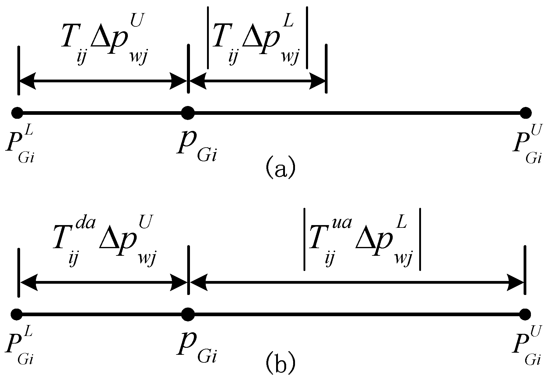
From the counterpart (26) and (27), the result of in (27) representing the worst case is included in solving the problem. The adjustment of ith dispatchable generator is determined by both the optimal solution of and the realization of . However, the upward and downward adjustment may not be equal. Suppose that and is close to the . In Figure 1a, the optimal solution of is dependent on the smaller downward adjustment, leading to a small upward adjustment . If the upward adjustment is optimized separately, the ability to provide upward adjustment could be large, as depicted in Figure 1b. Therefore, we adopt , and , instead of and to precisely describe the bidirectional adjustment of dispatchable generators. This can avoid a conservative estimation for the level of flexibility. The superscripts ua and da are short for upward adjustment and downward adjustment respectively. and would work if wind power is lower that the average level (i.e., ) while and would work in the case of .
Finally, the robust counterpart of the constraints (15)–(18) can be recast as follows:
where,
Positive variables , , , , , , , , , , , are introduced to formulate the robust couterpart. The functions in the right side of constraints (29), (31), (33) and (35) are embodied as the adjustable coefficients , and , are positive values, , and . The functions in (37) and (39) are reserved because and depend on elements in the line-bus power relational matrix .
The proposed optimization is reformulated by the objective (14), equality constraints (8) and (13), and the robust counterpart (28)–(39) of all inequality constraints. The choice of uncertainty budget would impose different restrictions on the variability of uncertain elements. = means no restriction is imposed on the size of uncertainty set . This is the most conservative case because the maximum range of variability in wind power is considered. Decreasing would decrease the conservativeness, resulting in smaller optimal objective value compared with that obtained in the most conservative case. = 0 would result in solutions without uncertainty. Therefore, decision makers can adjust to capture the level of flexibility.
4. Results
The proposed model is applied to a modified Garver six-bus system and a provincial power system in the northeastern region in China for an effectiveness evaluation and practical application. The formulations are implemented with MATLAB (R2011b, Mathworks, Natick, MA, USA) and solved with CPLEX (12.4, IBM, Armonk, NY, USA) on an Intel Core i5 CPU running at 2.90 GHz with 4 GB of RAM.
4.1. Modified Garver Six-Bus System
Four wind farms are considered in this modified Garver six-bus system, as depicted in Figure 2. The parameters of wind farms are shown in Table 1. The transmission capacity, parameters of generators and load data are available in [27]. Load data are expanded by multiplying them with 1.25. Assume all bus nodes can allocate energy storage. All generators are assumed as flexible units. In order to account for the most conservative scenario of uncertainties, . Three cases are designed to evaluate the requirement of energy storage under different levels of flexibility. Here G, W, E, B, N in all figures and tables denote generators, wind farms, energy storage, branches(transmission lines) and bus nodes respectively, followed by the number of bus node in the system.
4.1.1. Case 1: Limited Transmission Capacity
In this case, the flexibility provided by generators is sufficient, employing the operational range shown in Table 2. In the initial topology, there are two lines connecting bus nodes 3 and 5. In this situation, an energy storage with a power capacity of 21.2 MW is required at bus node 5. When accommodating the variation from wind generation, the maximum output of G1, minimum output of G3 and the transmission capacity of branch 3–5 could reach the bound value. These tight constraints are highlighted with overstriking numbers in Table 3. If one more line is added between node 3 and 5, results show that there is no need to allocate energy storage. Compared to the initial network with B3-5 = 2, no tight constraints exist in the new network presented in Table 3, which matches the result of no requirement of energy storage. After strengthening the transmission capacity of branch 3-5, G3 can provide more power to alleviate the stress of G1 and G6 in power balance. The limited transmission capacity constrains the power delivery of generators, thus energy storage is required at the terminal of line B3-5 to provide extra flexibility and relieve the transmission stress.
This case refers to the situations where weak links exist in the transmission network. The network expansion may somewhat lag behind the generation expansion, especially the rapidly integration of renewable energy projects. An appropriate energy storage allocation is shown to help accommodate renewable generation and postpone the transmission network expansion.
4.1.2. Case 2: Limited Flexibility From Existing Generators
In this case, the flexibility provided by transmission network is sufficient. All lines in Figure 2 are expanded to relax transmission network constraints. A limited level of flexibility from existing generators is considered, applying the operational range shown in Table 4. With a limited operation range of dispatchable generators, a shortage of 20 MW adjustable capacity is experienced. The power capacity of energy storage is distributed equally in all candidate nodes shown in Table 5 because of the relaxed transmission network constraints.
The average output of generators are intended for power balance. In Table 6, the average output form generators are close to their upper bound values, significantly limiting the available upward adjustable capacity. Thus the downward variation from wind power is difficult to accommodate by existing generators, resulting in the need of energy storage to provide additional flexibility. If a quantity of 20 MW is added to the maximum generation for any generator, there is no need for energy storage. The shortage of 20 MW can be compensated by energy storage. This case indicates that a small amount of power capacity of the energy storage could be helpful in situations where the flexibility from conventional generators is limited by other constraints, such as the heat demand constraint.
4.1.3. Case 3: Limited Transmission Capacity and Flexibility from Existing Generators
This case is established based on the assumptions in the above-mentioned cases. The limited operation range presented in Table 4 and the transmission network in Figure 2 are employed in case 3. Results show that the energy storage with the power capacity of 37.4 MW is required at bus node 5 when = 4. Limited transmission capacity and generators’ flexibility increase the need for power capacity of energy storage compared with results obtained from cases 1 and 2.
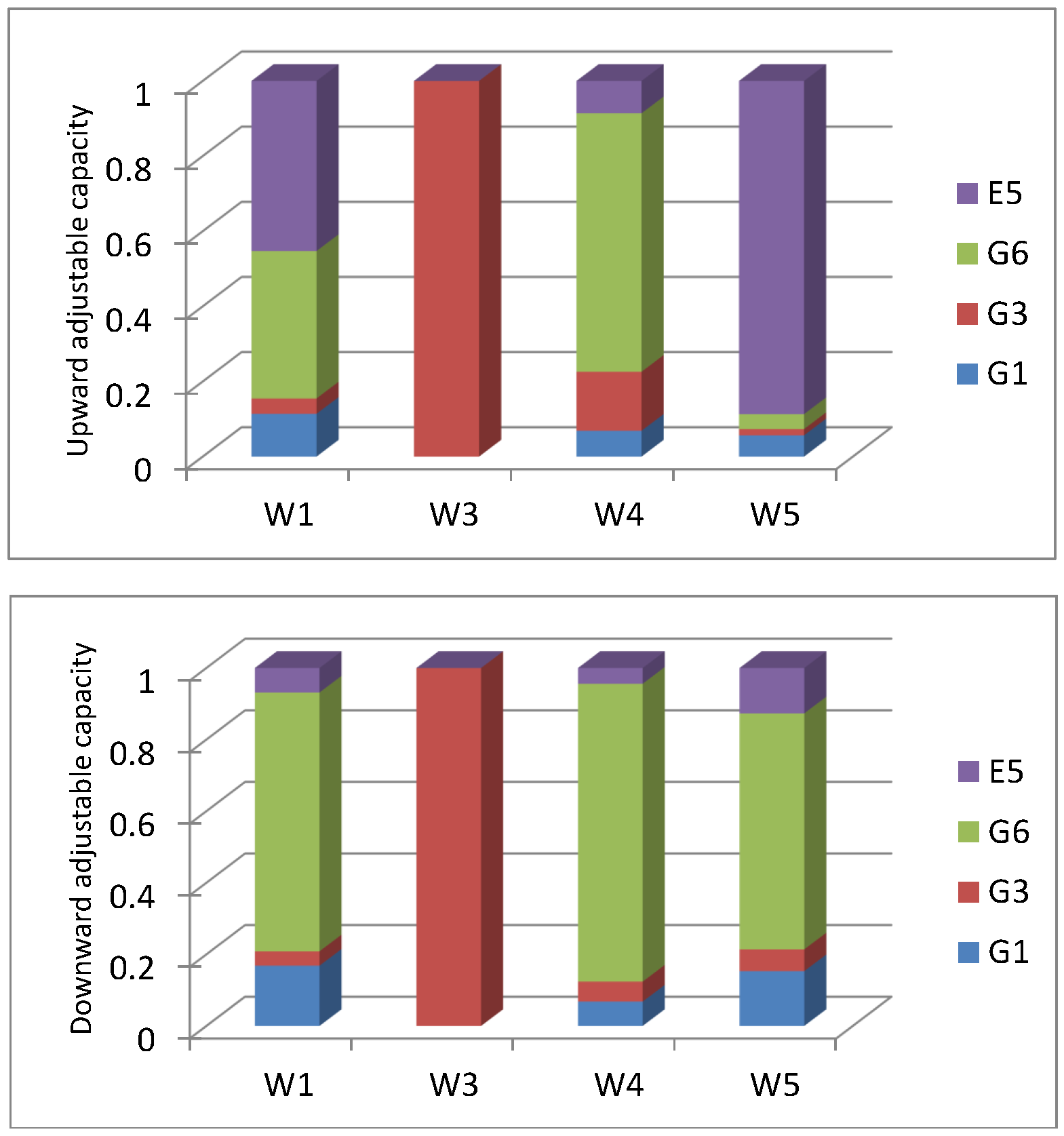
The adjustable coefficients for dispatchable generators, , , and energy storage at bus node 5, , , are optimized. The relationship modeled in the constraint (8) is presented by the column in Figure 3, indicating which flexible resource is available to accommodate wind power variation. The energy storage is mainly employed to provide upward adjustable power as the upward adjustable power from G1 and G6 are limited, according to Table 7. The downward adjustable power is primarily provided by dispatchable generators. Maximizing the utilization of the flexibility provided by existing generators enables the minimal requirement of energy storage. The importance of introducing separate coefficients to model the upward and downward adjustment is explained, otherwise, a greater need for energy storage could be expected.
The impacts of the robust budget on the power capacity of energy storage are discussed. The proposed model is simulated when decreases from 4 to 0 by a 0.1 step. The reducing requirement of the power capacity of energy storage with respect to is illustrated in Figure 4 in a blue dotted line. = 4 denotes the most conservative case where the maximum power capacity of energy storage is solved. Decreasing narrows the size of uncertainty sets, relaxing the conservativeness of the optimal solutions obtained from the robust counterpart. Thus, an evaluation of the robustness of solutions is required by employing the Monte Carlo simulation. Firstly, a set of 10,000 scenarios for the realization of wind power are generated. The shape parameter of Weibull distribution is 1.9622 for all wind farms, and the scale parameters are 8.3, 9.9, 8.4, 11.7 for W1–W5 respectively [28]. The parameters of the wind turbine are = 3 m/s, = 10.5 m/s and = 25 m/s considering the maximum power point tracking control [29,30]. Then, these scenarios are applied to evaluate the probability of violating constraints (15)–(18) under different robust budget parameters, presented in a red dotted line in Figure 4. Allocating a smaller size of energy storage could save the total investment, but the integration of wind power could not be ensured because of the decreased robustness. A tradeoff between the requirement of energy storage and the integration of variable renewable generation can be reached by controlling the value of the robust budget.
4.2. A Provincial Power System in China
The proposed model is applied to the Liaoning provincial power system, employing the actual data from the year of 2011. The case is composed of 250 bus nodes, 368 transmission lines (including 500 kV and 220 kV transmission lines) and 70 dispatchable generators. The total load power considered in the case is 22,021 MW. A snapshot of the 500 kV transmission network is presented in Figure 5. For all generators, the maximum output level is set as 1. The minimum output level is set as 0.5, 0.6 and 0.8 for generators with capacities more than 300 MW, between 100 MW and 300 MW, and less than 100 MW respectively. There are eight inter-regional transmission lines connecting the Liaoning provincial power grid with the North China regional power grid, Inner Mongolia and Jilin provincial power grids. The connecting bus nodes are considered as inflexible generators and loads depending on the direction of power exchange. The transmission capacities of each 500 kV and 220 kV transmission line are assumed as 1600 MW and 352 MW, respectively. The great physical potential for wind energy in the Liaoning province is distributed in four areas, shown in Figure 5. Seven wind farms with a large installed capacity are selected and the information is presented in Table 8. The wind power capacity totals 1789.3 MW, accounting for 8% of the load. The robust budget for this case is set as 7 in order to consider the most conservative case.
In this case, the energy storage with a power capacity of 48.5 MW is required at bus node 219 when considering transmission network constraints. The wind farm ZB is grid-integrated at the same bus node 219, accommodated by the required energy storage. The maximum absolute value of power flow through transmission line B97-219 could reach the transmission capacity when considering the impacts of uncertain wind power, shown in the Table 9. If relaxing the transmission capacity, there is no need for energy storage. However, the transmission capacity of transmission line B97-219 would increase to at least 400.5 MW according to the maximum absolute value of power flow. The power capacity of energy storage is equal to the difference between the maximum absolute values of power flow. According to the 220 kV transmission network of the Zhangwu District, two large-scale wind farms (ZB at bus node 219 and ZD at bus node 221) are grid-integrated through two transmission lines (B96-97). Results in Table 9 indicate that the flexibility provided by dispatchable generators is sufficient but limited by the transmission capacity of B96-97 in areas with intensive wind power. The probability of high level of generation from wind farms in the Liaoning province is not very large [31]. Thus, allocating energy storage with a small power capacity for large-scale wind farms could help store over-generation from wind farms that is otherwise curtailed. The stored energy can export to the power grid when the available wind generation is not great and the transmission network constraint is not bounded. The power capacity of energy storage can be reduced if a small robust budget is considered to relax the conservativeness.
5. Conclusions
The proposed approach provides a convenient way to determine the power capacity and installing location of energy storage to help accommodate the variable renewable generation. Through simulation analysis carried out with a modified Garver 6-bus system and the Liaoning provincial power system in China, the following conclusions can be drawn:
- (1)
- The need for energy storage is expected when the existing level of flexibility is limited by either transmission network constraint or generators’ operational range.
- (2)
- The optimal adjustable coefficients for dispatchable generators and energy storage indicate contributions of various flexible resources to variability accommodation. The abilities of each dispatchable generator to adjust power output upward and downward with respect to the asymmetric variability from renewable generation are modeled separately, employing two different adjustable coefficients. This modeling approach ensures the utilization of available flexibility of each generator can be maximized, thus minimizing the requirement of power capacity for energy storage.
- (3)
- An optimal allocation of energy storage, including the minimal power capacity and grid-integrated bus node, can be obtained through the proposed model. The increase of transmission capacity is expected to be 30 times more than the power capacity of energy storage. The allocated energy storage with a small amount of power capacity can complement the insufficiency of flexibility, thus the transmission network and generation expansion could be unnecessary.
- (4)
- Higher penetration level of variable renewable energy in transmission power grids could be expected. Given the priority of renewable generation, a sufficient level of flexibility that can be provided by existing flexible resources and employed to accommodate variable renewable generation is important. Employing the proposed method, the minimal need for energy storage can be obtained considering the high investment cost of energy storage. From this aspect, our approach can not only be employed as a planning tool to determine the allocation of energy storage, but could also be applied as an assessment tool to quantify the level of inflexibility employing the need for energy storage as an indicator.
Acknowledgments
This work is supported by National Key Research and Development Program of China (2016YFB0900400, 2016YFB0900403) and China Postdoctoral Science Foundation (2016M590693).
Author Contributions
Xingning Han, Xiaomeng Ai and Jinyu Wen conceived the idea and proposed the optimization model, Xingning Han and Shiwu Liao introduced the approach for solutions, Wei Yao collected the data, Xingning Han, Shiwu Liao and Xiaomeng Ai performed simulations and analyzed the data. All authors discussed results and contributed to writing the paper.
Conflicts of Interest
The authors declare no conflict of interest.
References
- Lannoye, E.; Flynn, D.; O’Malley, M. Evaluation of Power System Flexibility. IEEE Trans. Power Syst. 2012, 27, 922–931. [Google Scholar] [CrossRef]
- Zhang, L.; Capuder, T.; Mancarella, P. Unified Unit Commitment Formulation and Fast Multi-Service LP Model for Flexibility Evaluation in Sustainable Power Systems. IEEE Trans. Sustain. Energy 2016, 7, 658–671. [Google Scholar] [CrossRef]
- Chandler, H. Harnessing Variable Renewables: A Guide to the Balancing Challenge; Technical Report; International Energy Agency: Paris, France, 2011. [Google Scholar]
- Zhang, N.; Lu, X.; McElroy, M.B.; Nielsen, C.P.; Chen, X.; Deng, Y.; Kang, C. Reducing curtailment of wind electricity in China by employing electric boilers for heat and pumped hydro for energy storage. Appl. Energy 2016, 184, 987–994. [Google Scholar] [CrossRef]
- Liu, Y.; Hou, X.; Wang, X.; Lin, C.; Guerrero, J.M. A Coordinated Control for Photovoltaic Generators and Energy Storages in Low-Voltage AC/DC Hybrid Microgrids under Islanded Mode. Energies 2016, 9, 651. [Google Scholar] [CrossRef]
- Lotfy, M.E.; Senjyu, T.; Farahat, M.A.F.; Abdel-Gawad, A.F.; Yona, A. A Frequency Control Approach for Hybrid Power System Using Multi-Objective Optimization. Energies 2017, 10, 80. [Google Scholar] [CrossRef]
- Baun, M.; Awadallah, M.A.; Venkatesh, B. Implementation of load-curve smoothing algorithm based on battery energy storage system. In Proceedings of the 2016 IEEE Canadian Conference on Electrical and Computer Engineering (CCECE), Vancouver, BC, Canada, 15–18 May 2016. [Google Scholar]
- Liu, W.; Sun, L.; Lin, Z.; Wen, F.; Xue, Y. Multi-objective restoration optimisation of power systems with battery energy storage systems. IET Gener. Transm. Distrib. 2016, 10, 1749–1757. [Google Scholar] [CrossRef]
- Yao, W.; Jiang, L.; Wen, J.Y.; Wu, Q.H.; Cheng, S.J. Wide-area damping controller for power system inter-area oscillations: A networked predictive control approach. IEEE Trans. Control Syst. Technol. 2015, 23, 27–36. [Google Scholar] [CrossRef]
- Yao, W.; Jiang, L.; Fang, J.K.; Wen, J.Y.; Cheng, S.J.; Wu, Q.H. Adaptive Power Oscillation Damping Controller of Superconducting Magnetic Energy Storage Device for Interarea Oscillations in Power System. Int. J. Electr. Power Energy Syst. 2016, 78, 555–562. [Google Scholar] [CrossRef]
- Khani, H.; Zadeh, M.R.D.; Hajimiragha, A.H. Transmission Congestion Relief Using Privately Owned Large-Scale Energy Storage Systems in a Competitive Electricity Market. IEEE Trans. Power Syst. 2016, 31, 1449–1458. [Google Scholar] [CrossRef]
- Kang, C.; Chen, X.; Xu, Q.; Ren, D.; Huang, Y.; Xia, Q.; Wang, W.; Jiang, C.; Liang, J.; Xin, J.; et al. Balance of Power: Toward a More Environmentally Friendly, Efficient, and Effective Integration of Energy Systems in China. IEEE Power Energy Mag. 2013, 11, 56–64. [Google Scholar] [CrossRef]
- Liu, J.; Zhang, L. Strategy Design of Hybrid Energy Storage System for Smoothing Wind Power Fluctuations. Energies 2016, 9, 991. [Google Scholar] [CrossRef]
- Liu, Y.; Du, W.; Xiao, L.; Wang, H.; Bu, S.; Cao, J. Sizing a Hybrid Energy Storage System for Maintaining Power Balance of an Isolated System With High Penetration of Wind Generation. IEEE Trans. Power Syst. 2016, 31, 3267–3275. [Google Scholar] [CrossRef]
- Liu, J.; Wen, J.Y.; Yao, W.; Long, Y. Solution to Short-term Frequency Response of Wind Farms by Using Energy Storage Systems. IET Renew. Power Gener. 2016, 10, 669–678. [Google Scholar] [CrossRef]
- Masiello, R. Bottling Electricity Time to Get Real. IEEE Power Energy Mag. 2009, 7, 22–25. [Google Scholar] [CrossRef]
- Aly, M.M.; Salama, H.S.; Abdel-Akher, M. Power control of fluctuating wind/PV generations in an isolated Microgrid based on superconducting magnetic energy storage. In Proceedings of the 2016 Eighteenth International Middle East Power Systems Conference (MEPCON), Cairo, Egypt, 27–29 December 2016; pp. 419–424. [Google Scholar]
- Jin, J.; Xu, Y.; Khalid, Y.; Hassan, N.U. Optimal Operation of Energy Storage with Random Renewable Generation and AC/DC Loads. IEEE Trans. Smart Grid 2016. [Google Scholar] [CrossRef]
- Díaz-González, F.; Sumper, A.; Gomis-Bellmunt, O.; Villafáfila-Robles, R. A review of energy storage technologies for wind power applications. Renew. Sustain. Energy Rev. 2012, 16, 2154–2171. [Google Scholar] [CrossRef]
- Haghi, H.V.; Lotfifard, S. Spatiotemporal Modeling of Wind Generation for Optimal Energy Storage Sizing. IEEE Trans. Sustain. Energy 2015, 6, 113–121. [Google Scholar] [CrossRef]
- Baker, K.; Hug, G.; Li, X. Energy Storage Sizing Taking Into Account Forecast Uncertainties and Receding Horizon Operation. IEEE Trans. Sustain. Energy 2017, 8, 331–340. [Google Scholar] [CrossRef]
- Nguyen, N.T.A.; Le, D.D.; Moshi, G.G.; Bovo, C.; Berizzi, A. Sensitivity Analysis on Locations of Energy Storage in Power Systems With Wind Integration. IEEE Trans. Ind. Appl. 2016, 52, 5185–5193. [Google Scholar] [CrossRef]
- Ben-Tal, A.; Nemirovski, A. Robust solutions of Linear Programming problems contaminated with uncertain data. Math. Program. 2000, 88, 411–424. [Google Scholar] [CrossRef]
- Bertsimas, D.; Sim, M. The Price of Robustness. Oper. Res. 2004, 52, 35–53. [Google Scholar] [CrossRef]
- Dehghan, S.; Amjady, N.; Kazemi, A. Two-stage Robust Generation Expansion Planning: A Mixed Integer Linear Programming Model. IEEE Trans. Power Syst. 2014, 29, 584–597. [Google Scholar] [CrossRef]
- Kang, S.C. Robust Linear Optimization Using Distributional Information. Ph.D. Thesis, Boston University, Boston, MA, USA, 2008. [Google Scholar]
- Garver, L.L. Transmission Network Estimation Using Linear Programming. IEEE Trans. Power Appar. Syst. 1970, PAS-89, 1688–1697. [Google Scholar] [CrossRef]
- Yeh, T.H.; Wang, L. A Study on Generator Capacity for Wind Turbines Under Various Tower Heights and Rated Wind Speeds Using Weibull Distribution. IEEE Trans. Energy Convers. 2008, 23, 592–602. [Google Scholar]
- UnitedPower UP82/1500 Wind Turbine Characteristics. Available online: http://www.thewindpower.net/turbine_en_663_guodian_1500.php (accessed on 29 March 2017).
- Yang, B.; Jiang, L.; Wang, L.; Yao, W.; Wu, Q.H. Nonlinear Maximum Power Point Tracking Control and Modal Analysis of DFIG Based Wind Turbine. Int. J. Electr. Power Energy Syst. 2016, 74, 429–436. [Google Scholar] [CrossRef]
- Ai, X.; Wen, J.; Wu, T.; Lee, W.J. A Discrete Point Estimate Method for Probabilistic Load Flow Based on the Measured Data of Wind Power. IEEE Trans. Ind. Appl. 2013, 49, 2244–2252. [Google Scholar] [CrossRef]
Figure 1.
(a) Employing the same variable to model the upward and downward adjustment from ith generator; (b) Employing different variables, and , to optimize the upward and downward adjustment of ith dispatchable generator.
Figure 1.
(a) Employing the same variable to model the upward and downward adjustment from ith generator; (b) Employing different variables, and , to optimize the upward and downward adjustment of ith dispatchable generator.

Figure 2.
Topology of modified Garver 6-bus system.

Figure 3.
Upward and downward adjustable coefficients of dispatchable generators and energy storage to accommodate wind power.
Figure 3.
Upward and downward adjustable coefficients of dispatchable generators and energy storage to accommodate wind power.

Figure 4.
Power capacity of energy storage and the corresponding violation probability versus the robust budget.
Figure 4.
Power capacity of energy storage and the corresponding violation probability versus the robust budget.
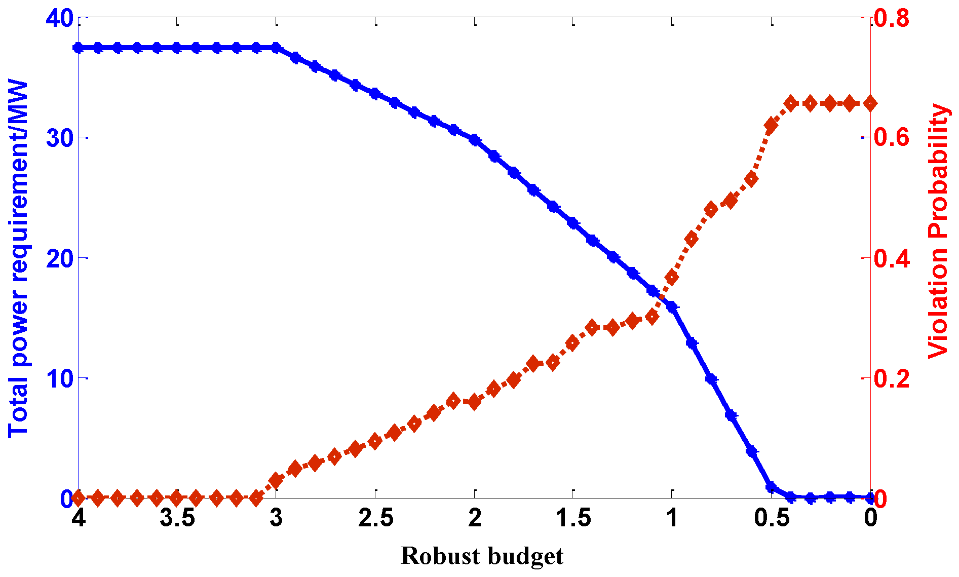
Figure 5.
Illustration of the transmission network of Liaoning provincial power grid.


Table 1.
Information of Wind Farms Integrated.
| Wind Farms | W1 | W3 | W4 | W5 |
|---|---|---|---|---|
| Capacity | 49.5 | 49.5 | 49.5 | 49.5 |
| Average Output | 20 | 25 | 20 | 30 |
| Minimum Output | 0 | 0 | 0 | 0 |
Table 2.
Operation Range of Generators (MW).
| Generators | Minimum Power Output | Maximum Power Output |
|---|---|---|
| G1 | 90 | 150 |
| G3 | 180 | 360 |
| G6 | 300 | 600 |
Table 3.
Power output from generators and power flow from transmission lines in case 1 (MW).
| B3-5 = 2 | Generators | Average Output | Range |
| G1 | 140.33 | 93.10–150.00 | |
| G3 | 203.63 | 180.00–347.78 | |
| G6 | 511.04 | 321.53–594.46 | |
| Branch | Transmission Capacity | Maximum Absolute Value | |
| B3-5 | 200 | 200.00 | |
| B3-5 = 3 | Generators | Average Output | Range |
| G1 | 123.10 | 92.70–147.56 | |
| G3 | 290.28 | 190.24–354.70 | |
| G6 | 441.62 | 315.60–589.21 | |
| Branch | Transmission Capacity | Maximum Absolute Value | |
| B3-5 | 300 | 294.71 |
Table 4.
Limited Operation Range of Generators (MW).
| Generators | Minimum Power Output | Maximum Power Output |
|---|---|---|
| G1 | 120 | 150 |
| G3 | 200 | 280 |
| G6 | 300 | 500 |
Table 5.
Power capacity of energy storage in case 2 (MW).
| Bus Node | 1 | 2 | 3 | 4 | 5 | 6 |
| Power Capacity of Energy Storage | 3.4 | 3.3 | 3.4 | 3.3 | 3.3 | 3.3 |
Table 6.
Power output from generators in case 2 (MW).
| Generators | Average Output | Range | |
|---|---|---|---|
| Minimum Value | Maximum Value | ||
| G1 | 141.38 | 121.36 | 150.00 |
| G3 | 261.65 | 205.8 | 280.00 |
| G6 | 451.97 | 315.01 | 500.00 |
Table 7.
Power output from generators and tight constraint on power flow of transmission line in case 3 (MW).
Table 7.
Power output from generators and tight constraint on power flow of transmission line in case 3 (MW).
| Generators | Average Output | Range |
|---|---|---|
| G1 | 144.65 | 121.58–150.00 |
| G3 | 233.14 | 200.68–278.00 |
| G6 | 477.21 | 316.61–500.00 |
| Branch | Branch Capacity | Maximum Absolute Value |
| B3-5 | 200 | 200.0 |
Table 8.
Information of wind farms.
| Integrated Node | 205 | 209 | 219 | 221 | 223 | 230 | 235 |
| Wind Farms | LH | TS | ZB | ZD | FB | LK | HP |
| Capacity (MW) | 198 | 99 | 400.5 | 346.5 | 300 | 346.3 | 99 |
| Average Output (MW) | 66 | 33 | 133.5 | 115.5 | 100 | 115.4 | 33 |
| Minimum Output (MW) | 0 | 0 | 0 | 0 | 0 | 0 | 0 |
| Location | Jinzhou | Wafang | Zhangwu | Zhangwu | Fuxin | Zhangwu | Wafang |
Table 9.
Results with and without Transmission Network Constraints.
| Case Description | Energy Storage | Max Absolute Value of Power Flow (MW) | |||
|---|---|---|---|---|---|
| Node | Power | B96-97 | B97-219 | B97-221 | |
| with network | 219 | 48.5 | 645.9 | 352 | 346.5 |
| without network | - | - | 2065.4 | 400.5 | 693 |
© 2017 by the authors. Licensee MDPI, Basel, Switzerland. This article is an open access article distributed under the terms and conditions of the Creative Commons Attribution (CC BY) license (http://creativecommons.org/licenses/by/4.0/).
Share and Cite
MDPI and ACS Style
Han, X.; Liao, S.; Ai, X.; Yao, W.; Wen, J. Determining the Minimal Power Capacity of Energy Storage to Accommodate Renewable Generation. Energies 2017, 10, 468. https://doi.org/10.3390/en10040468
AMA Style
Han X, Liao S, Ai X, Yao W, Wen J. Determining the Minimal Power Capacity of Energy Storage to Accommodate Renewable Generation. Energies. 2017; 10(4):468. https://doi.org/10.3390/en10040468
Chicago/Turabian StyleHan, Xingning, Shiwu Liao, Xiaomeng Ai, Wei Yao, and Jinyu Wen. 2017. "Determining the Minimal Power Capacity of Energy Storage to Accommodate Renewable Generation" Energies 10, no. 4: 468. https://doi.org/10.3390/en10040468
Note that from the first issue of 2016, this journal uses article numbers instead of page numbers. See further details here.