Article

Development of a Real-Time Virtual Nitric Oxide Sensor for Light-Duty Diesel Engines

Department of Mechanical and Aerospace Engineering, Seoul National University, 1 Gwanak-ro, Gwanak-gu, Seoul 08826, Korea
*
Author to whom correspondence should be addressed.
Energies 2017, 10(3), 284; https://doi.org/10.3390/en10030284
Submission received: 9 January 2017 / Revised: 10 February 2017 / Accepted: 21 February 2017 / Published: 1 March 2017

Abstract

:
This study describes the development of a semi-physical, real-time nitric oxide (NO) prediction model that is capable of cycle-by-cycle prediction in a light-duty diesel engine. The model utilizes the measured in-cylinder pressure and information obtained from the engine control unit (ECU). From the inputs, the model takes into account the pilot injection burning and mixing, which affects the in-cylinder mixture formation. The representative in-cylinder temperature for NO formation was determined from the mixture composition calculation. The selected temperature and mixture composition was substituted using a simplified form of the NO formation rate equation for the cycle-by-cycle estimation. The reactive area and the duration of NO formation were assumed to be limited by the fuel quantity. The model predictability was verified not only using various steady-state conditions, including the variation of the EGR rate, the boost pressure, the rail pressure, and the injection timing, but also using transient conditions, which represent the worldwide harmonized light vehicles test procedure (WLTC). The WLTC NO prediction results produced less than 3% error with the measured value. In addition, the proposed model maintained its reliability in terms of hardware aging, the changing and artificial perturbations during steady-state and transient engine operations. The model has been shown to require low computational effort because of the cycle-by-cycle, engine-out NO emission prediction and control were performed simultaneously in an embedded system for the automotive application. We expect that the developed NO prediction model can be helpful in emission calibration during the engine design stage or in the real-time controlling of the exhaust NO emission for improving fuel consumption while satisfying NO emission legislation.

1. Introduction

The NOx emissions from on-road vehicles have significant effects on the environment and human health [1]. Due to these impacts, there has been increasing demand for cleaner vehicles with progressively more stringent emission regulations. From the regulation point of view, diesel engines are unfavorable because of the NOx and smoke due to the diffusion combustion characteristics. Nevertheless, diesel engines have advantages in fuel economy and CO2 emissions as there is a greater margin [2] to satisfy the proposed and established greenhouse-gas emission standards [3], and therefore, researchers have shown interest in reducing NOx emissions from diesel engines.
There are two approaches used to reduce tail-pipe NOx emissions. One approach is changing the combustion concepts, such as low-temperature combustion using heavy exhaust gas recirculation (EGR) [4,5,6,7], and the second approach is using after-treatment devices, such as a lean NOx trap (LNT) and a selective catalytic reduction (SCR) [8,9]. The former concept requires more extensive research and effort compared to conventional diesel engines with respect to covering the full operating range and increasing the CO emission [10]. The latter has become essential in recent years to comply with stringent emission legislation. However, in both cases, there is a need for a real-time prediction tool to optimize the operation. Recently, car manufacturers have attempted to replace physical NOx sensors with virtual NOx sensors to reduce material costs and overcome the limited response time. Although this replacement is challenging, a virtual NOx sensor can be helpful in determining physical NOx sensor malfunction or controlling after-treatment devices [11].
A common approach to the virtual NOx sensor can be categorized as physics-based, gray box, and black box models. The terms physics-based and phenomenological, gray box and semi-empirical, and black box and empirical are often used interchangeably, although the scope of the terms phenomenological and semi-empirical varies among authors [11,12]. Regardless of how they are defined, the physics-based and gray box models are physically related. The proposed models based on the physical and chemical relations show more reliable results with environmental perturbations, such as different engines, EGR, and rail and intake pressure variations [11,13,14]. For this reason, many studies of virtual NOx sensors have been performed from physical and phenomenological points of view [12,14,15,16,17,18,19,20,21]. Egnell proposed a multi-zone model of combustion diagnostics based on heat release, which he used to calculate the amount of nitric oxide (NO) that formed during the combustion process [15]. Andersson et al. modified Egnell’s research to produce an efficient algorithm using tables with chemical equilibrium data [14]. Arrègle et al. investigated a sensitivity analysis for additionally developed NOx production estimation model and reported that the admitted fresh air measurement and the temperature in the intake manifold were critical input parameters for the calculation of the NOx formation rate [17]. Seykens et al. developed an extended NO and soot production model for advanced heavy-duty diesel engine combustion cycles, which was validated using experimental data [18]. Willems et al. subsequently applied the model [17] to cylinder pressure-based controls in a heavy-duty diesel engine with a high EGR rate [19]. Hegarty et al. employed a semi-empirical model in their approach to the dynamic NOx production modeling of a diesel engine. They correlated the model with experimental results using Zeldovich’s coefficient map [20]. Finesso et al. developed a zero-dimensional combustion predictive model, which was used in a NOx production estimation model [21].
Although previous research has produced reliable NOx production estimates, some limiting factors exist, such as the complexity of the model, which is detrimental to use in real-time applications, the need for many calibration constants, ignoring the effect of the pilot injection combustion, the rough approximation of the NOx based on NO mechanisms, and lack of distinguish between the NO or NO2 portion in the NOx emission.
Furthermore, according to previous research, the diesel engine exhaust gas treatment systems are closely coupled with the NO or NO2 portion in the NOx emission [22], and distinguishing the fraction of NO and NO2 in NOx can be essential in the design and in the exhaust of after-treatment systems. Likewise, favorable soot oxidation in diesel particulate filters (DPF) is plentiful in the case of NO2 but not for NO [23]. In addition, the conversion of NO to NO2 is important in LNT [24], and the NOx conversion rate is affected by the NO2 portion in the NOx in the SCR [25].
The portion of NO2 in the NOx of compression engine exhaust is known to be in order of 10%–30% [26] or more [27] depending on conditions. Based on current understanding, the majority of NO2 is converted from the NO [26,27,28,29]. The experiment results of the previous study shows that the NO2/NOx ratio can be simply expressed as a function of NO and by using the fact, NO2 or NOx was predicted from the NO using NO to NO2 or NOx 1-dimensional fitting map [30]. Moreover, NO still predominantly contributes exhaust NOx at higher loads [27]. Thus, knowing an exhaust NO emission could be a very important foundation for reducing the total NOx in diesel engines.
In this paper, a zero-dimensional, semi-physical, cycle-by-cycle NO estimation model with low calibration demands was developed. The model considers a spatial correction based on physical phenomena, such as the pilot burned mixing prior to the main injection, major NO formation area variation with related parameter changes, and the concentration correction based on the diffusion combustion characteristics to enhance extrapolation capability. To investigate the feasibility of the NO prediction model in real-time applications, the model was implemented in an embedded system (ES-1000, ETAS). The implemented model was suitable for both NO estimation in the WLTC and NO emission control during engine operation. Furthermore, real-time NO emission control was achieved by changing the main injection timing with a limited value for the combustion stability.

2. Experimental Setup and Conditions

2.1. Test Engine

A 1.6-L and a 2.2-L four cylinder light-duty diesel engine were selected to verify the model. Both engines were equipped with a turbocharger and a common-rail injection system with the same solenoid-type injector. In addition, the compression ratios for both engines were 17.3 and 16, respectively. The core specifications of engines are described in Table 1.

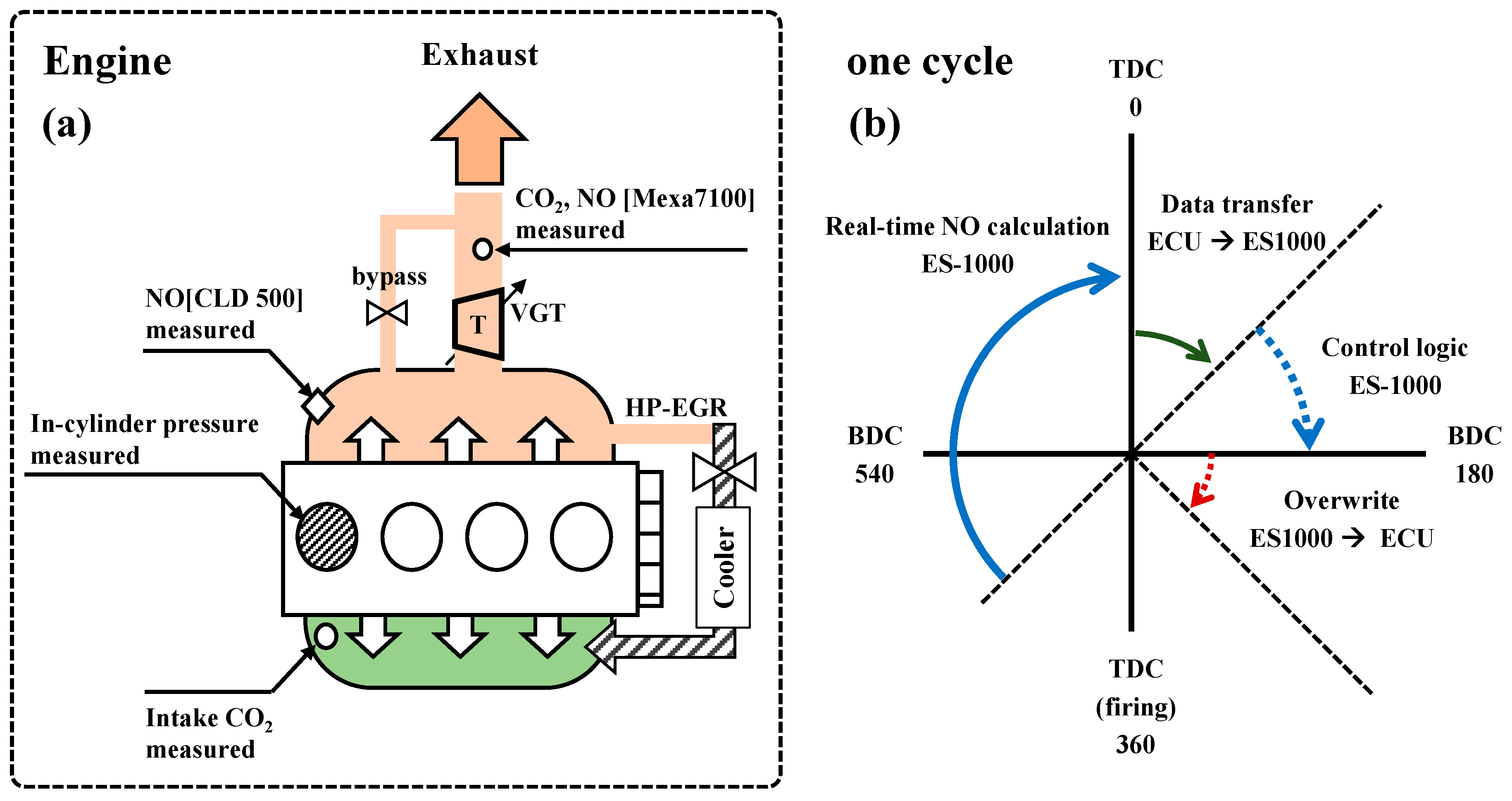
2.2. Experimental Setup

The engine test bed was connected to a 340 kW AC dynamometer (DynoDur, AVL, Graz, Austria), which was capable of steady-state operations and mirroring various homologation cycles through a controller (PUMA OPEN 1.3.2 automation system, AVL). During the experiments, the engine coolant and fuel temperature were maintained at 85–90 °C and 40 °C, respectively, to imitate vehicle conditions at room temperature.
The test engines were commercially produced engines, and the ETK-ECU interface was connected to PC software (Version 7.0, INCA, ETAS, Stuttgart, Germany) that allowed for the monitoring of the installed sensor signals and changing the major engine control parameters, such as the EGR, the rail pressure, the main injection timing and the boost pressure.
A glow plug type piezoelectric sensor (6056A, Kistler, Sindelfingen, Germany) was mounted on one of the cylinders, as indicated in Figure 1a, to take into account the real-time in-cylinder pressure data. The acquired in-cylinder pressure was pegged by the absolute boost pressure from the ECU and the top dead center (TDC) position is determined from combustion analyzer (KiBOx, Kistler). Once the TDC position was determined, it was saved in the ES-1000 before performing the engine-out NO calculation.

2.2.1. Engine-Out NO Measurement

The engine-out NO was measured using two pieces of equipment: an exhaust gas analyzer (MEXA-7100DEGR, HORIBA, Kyoto, Japan) during steady-state engine operation and a fast NO analyzer (CLD-500, Cambustion, Cambridge, UK), which is used for the cycle-by-cycle real-time NO measurement during homologation cycle operations. A fast NO analyzer has a fast response time (2 ms) compared with the MEXA-7100DEGR (900 ms). The sampling probe of the fast NO analyzer was installed at the confluence of the exhaust gas where the distance to the exhaust valve was minimized to reduce the sampling delay.

2.2.2. Real-Time Calculation and Control of Engine-Out NO

Rapid prototyping hardware (ES1000, ETAS) and integration software (ASCET, ETAS) were selected to evaluate the prediction model’s potential for real-time application. The ES1000 allows for the extension of its functions using interface boards, such as an ETK interface board (ES1232-A, ETAS), an analog/digital board (ES1303, ETAS) and a simulation/system controller board (ES1135, ETAS). The built-in engine sensor signals were delivered to the ES1000 in real time via the ETK interface board, and the A/D board integrated the different analog sensor signals, such as the pressure sensor and the gas analyzer signals, into the ES1000. The prediction model and the NO emission control logic were implemented in the simulation/system controller board (ES1135) and were especially developed for use in automotive applications. All calculations were conducted only using the computing power in the ES1135 board, and the results were monitored using a PC. As illustrated in Figure 1b, the entire process of the NO estimation and the NO control can be executed in a cycle. The first step is data exchange from the ECU to the ES1000, such as the engine speed, the air/fuel ratio (AF), and the injection timing.
After engine operating parameters are inserted from the ECU, the control logic calculates the appropriate injection timing for the target NO emission and overwrites the variable over 90 degrees of the crank angles. The process for controlling the engine-out NO is represented as dotted arrows in Figure 1b, and the process can be omitted when only predicting the engine-out NO. The NO estimation process is scheduled to be completed within a half of a cycle including the data exchange process, as shown by the solid arrow in Figure 1b. It should be noted that the estimated NO is matched in the present cycle while a previous cycle’s estimated NO value is used for control. Table 2 reports available data for the evaluation of measurement errors and expanded uncertainties. The calculation of the uncertainties were based on [31] assuming a level of confidence of 95%.

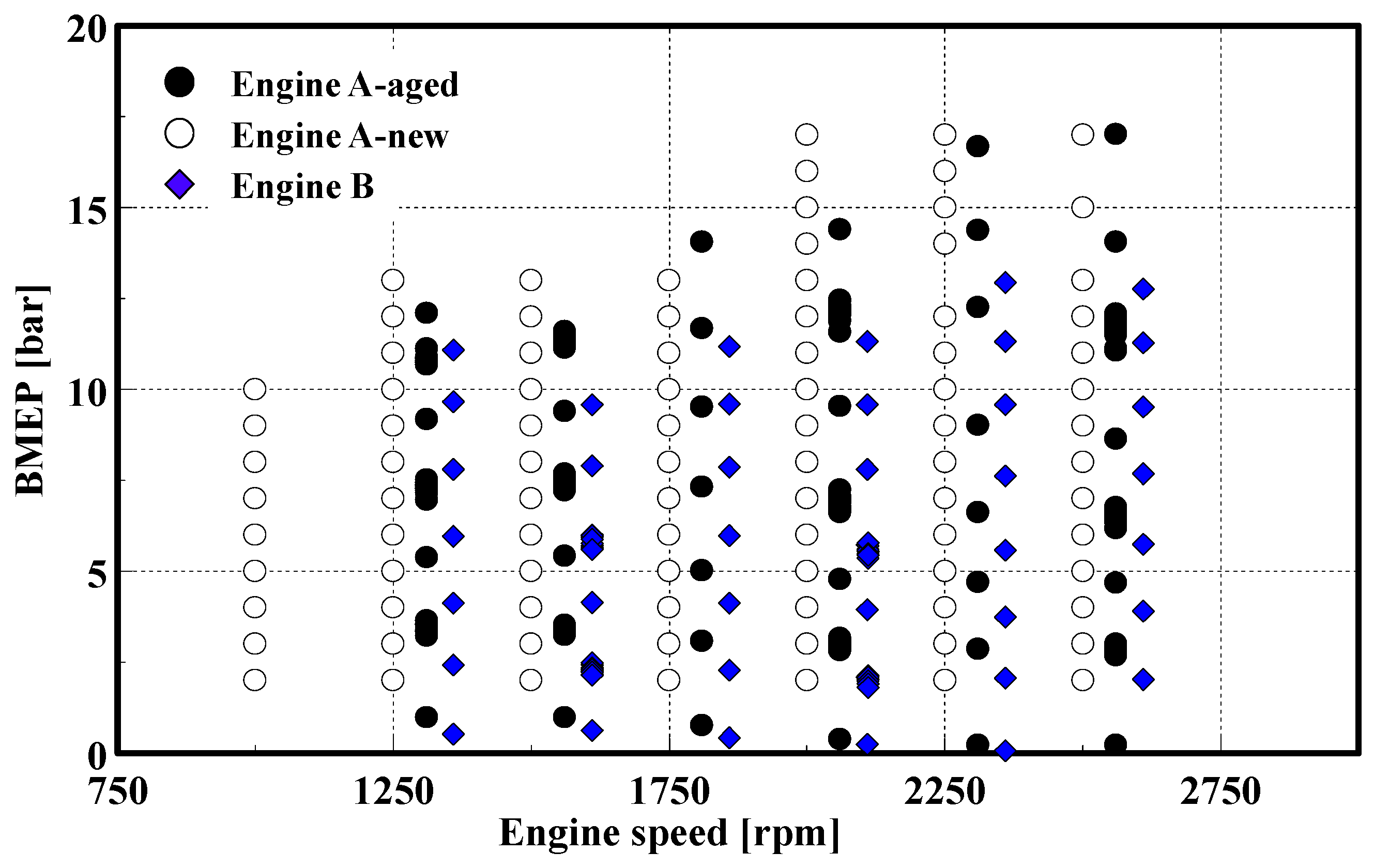
2.2.3. Experimental Conditions

The research in this paper was mainly performed with engine A-aged, and this engine was aged for more than 500 h using various conditions regardless of steady and transient operation in the range as follows. The steady-state operation conditions were an engine speed that ranged from 1000 to 2500 rpm with a BMEP of less than 20 bar. The entire WLTP cycle can be covered in the representative operation points, and setting the BMEP to a low value between 0 to 2 bar can reflect more rapid acceleration and deceleration conditions. The described steady-state test sets were organized as shown in Figure 2. As shown in the figure, three different engines with various points were used to verify the model’s robustness. The clusters of operation points are formed because the parameters, such as the EGR, the injection timing, the boost pressure, and the rail pressure, were varied to compare a typical engine operating map. More details of the typical conditions and sweep spacing are shown in Table 3.
In this paper, the WLTP cycle, which is known as a homologation cycle in Europe, was selected to investigate the real-time predictability of the model. The velocity profile for the entire cycle was converted to an equivalent engine speed and torque profile to simulate the dynamic test bench.
The reliability of the model was demonstrated using many different methods. First, the proposed model was applied to three different engines (engine A-aged, engine A-new and engine B) with two types, as described in Table 3 and Figure 2. Second, the data programed in the ECU was deviated to mimic the engine’s built-in sensor drift or actuator movement change due to aging. Last, the exhaust gas was bypassed, as shown in Figure 1a, to create hardware malfunction circumstances. More detailed information about the model robustness test conditions are shown in the section covering the model robustness validation.

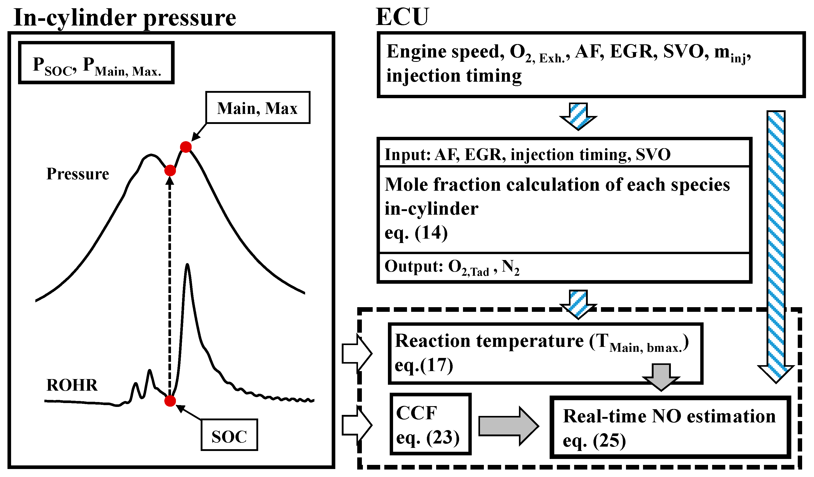
3. Description of the Real-Time NO Estimation Model

The preferable requirements for a real-time model are low computational cost, no calibration requirement, and the ability to be extrapolated outside of the calibration range. To meet these conditions, the inputs of the proposed model are restricted to the in-cylinder pressure information and the data available from the ECU. The in-cylinder pressure information can be altered using virtual pressure sensors or models but only the measured pressure is used in the results for a full discussion of the NO estimation model. The whole process of NO estimation is briefly structured in Figure 3, and more details of each process will be described in the sub-sections of this section.
The thermal NO mechanism, which is a super-extended Zeldovich mechanism, takes into account the good extrapolation capability. The three representative reactions are shown as follows:
O + N 2 NO + N
N + O 2 NO + O
N + OH NO + H
The equilibrium assumption [26] enables the simplification of the NO formation rate:
d [ NO ] d t = 6 × 10 16 T 1 / 2 exp ( 69090 T ) [ O 2 ] e 1 / 2 [ N 2 ] e   mol / cm 3 · s
where T is the gas temperature, and the square brackets are the molar concentrations of the corresponding species. The []e is the equilibrium concentration for a given reaction. Note that the given rate expression is the correlated molar formation of NO and should be considered when using this correlation. As shown in Equation (1), the strong dependence of the NO formation rate on the temperature is evident, and therefore, determination of the gas composition, which depends on the in-cylinder temperature, is a key issue when developing the model.

3.1. Determination of the Adiabatic Flame Temperature

Most of the NOx prediction models take into account the adiabatic flame temperature [11] in the calculation of the burned zone temperature. When calculating the adiabatic flame temperature, it is reasonable to consider the dissociation effect of the combustion products or to correct the temperature due to heat transfer [32]. However, none of these studies account for the gas composition change due to multiple injections, as adopted by most diesel engines, although the adiabatic flame temperature is related to the composition of the gases [33]. The combustion of hydrocarbon fuel is modeled as a single-step reaction to calculate the gas concentrations:
C x H y + λ γ ( O 2 + ψ N 2 ) + E G R ( a O 2 + b N 2 + c CO 2 + d H 2 O ) a O 2 + b N 2 + c CO 2 + d H 2 O
a = γ ( λ 1 ) / ( 1 E G R )
b = γ λ ψ / ( 1 E G R )
c = x / ( 1 E G R )
d = y / ( 2 ( 1 E G R ) )
where λ is the air excess ratio given by the ECU, γ = x + y / 4 , and ψ is the molar N/O ratio (3.773 for air). The EGR in Equation (2) is the EGR fraction that is obtained from inherent model in the ECU. From Equation (2), the unburned gas composition in moles can be calculated as follows:
n O 2 = γ + γ ( λ 1 ) / ( 1 E G R )
n N 2 = γ λ ψ / ( 1 E G R )
n CO 2 = x · E G R / ( 1 E G R )
n H 2 O = y · E G R / ( 2 ( 1 E G R ) )
In the case of pilot injection burn, the burned gas should be located at a position that affects the entrainment of the main injection [34], and therefore, the unburned gas composition deduced from Equations (7) to (10) cannot be directly used for the adiabatic flame temperature calculation. To help understand the composition change before the main injection event, computational fluid dynamics (CFD) analysis was examined in the reference condition and is shown in Figure 4. The computations were performed by the commercial CFD software Star-CD version 4.22 with combustion model ECFM-3Z [35], and a 1/7 sector mesh was generated with the ES-ICE toolkit. The mesh consisted of 67,000 cells at the BDC and 12,000 cells at the TDC with an extrusion method applied near the wall layer. For the boundary conditions, a cyclic boundary condition was applied to both sides in the azimuthal direction while all other regions had wall boundary conditions with a non-slip condition. Thermal boundary conditions for head, piston, and liner were fixed 430 K, 440 K, and 420 K respectively. The more details of the CFD simulation can be found in [36].
The CFD results in Figure 4a reveal that, before main injection, only a limited in-cylinder charge is consumed with an accompanying change in the local gas composition. The mixture fraction (Z) [37] was used to describe the portion that did not join the combustion, and Z = 0.01 was selected for the visualization.
Moreover, the injection of the main fuel coinciding with the local changed area is observed, as shown in Figure 4b. To capture the transformation of the in-cylinder condition before the main injection, the air availability ( α ) is introduced and is treated as a function of the quantity of fuel injected before the main injection, the swirl ratio, the engine speed and the dwell time (time interval between the end of pilot1 injection and start of main injection). Previous research has shown that the swirl promotes mixing between the air charge and the injected fuel and also affects the spray penetration and spreading [26]. It is obvious that the local gas composition continuously varies after the pilot injected fuel is burned because it mixes with the surroundings, and the characteristic time for the mixing is selected as the dwell time:
α = γ δ ω
ω ( 0 < ω 1 ) = scale   adjustment   of   ( swirl   ratio * Dwell   time   ( D T ) * engine   speed   ( r p m ) )
Equation (11) shows the air availability, which consists of ECU accessible parameters. The delta ( δ ) is a constant that is multiplied along with γ   to express that the air availability is proportional to the injected fuel amount. Throughout the calculation, δ was fixed at 8, which is appropriate for the minimum air mass condition that was tested in this paper. The swirl factor ( ω ) is defined as product of the swirl ratio, the dwell time and the engine speed to create a non-dimensional constant, and the maximum value in the experimental case was set to 1 for the largest effect. Including the air availability concept, the gas composition change due to the fuel burn can be expressed in a single-step reaction equation as follows:
C x H y + α ( O 2 + n N 2 O 2 n o r m . N 2 + n CO 2 O 2 n o r m . CO 2 + n H 2 O O 2 n o r m . H 2 O ) ( α γ ) O 2 + α · n N 2 O 2 n o r m . N 2 + ( x + α · n CO 2 O 2 n o r m . ) CO 2 + ( y 2 + α · n H 2 O O 2 n o r m . ) H 2 O
where subscript n O 2 n o r m . denotes the gas composition calculated in moles from Equation (8) through (10) divided by Equation (7), respectively. The gas concentration ratio, which considers the pilot injection burning and the mixing between each gas at the main injection timing, can be re-organized as Equation (14):
O 2 : N 2 : CO 2 : H 2 O = ( α γ ) : α · n N 2 O 2 n o r m . : ( x + α · n CO 2 O 2 n o r m . ) : ( y 2 + α · n H 2 O O 2 n o r m . )
A database of the adiabatic flame temperature was built from 220 simulation results for various operating conditions that were identical to engine A-aged in the experimental conditions section using Chemkin-IV. With respect to the fact that the dissociation effects are important, when creating the adiabatic flame temperature database, the burned combustion products were assumed to be the main combustion species and species relevant for NO formation: O2, N2, CO2, H2O, CO, H2, H, OH, O, N, NO and N2O,. To calculate the appropriate adiabatic temperature for the real-time model, a second-order formula was derived from the database. The final form of the equation used to calculate the adiabatic temperature is expressed as Equation (15):
T a d = 3312 + 22770 × O 2 _ a d + 6.638 × T S O C [ K ] 18150 × O 2 _ a d 2 10.48 × O 2 _ a d × T S O C [ K ] 0.002364 × T S O C [ K ] 2
O2_ad is the mole fraction of O2 in Equation (14), which includes the physical compensations of the gas composition change and mixing due to the fuel burn and swirl. TSOC is the temperature when the main combustion starts and is calculated from the ideal gas equation as follows.
T S O C = P S O C V S O C M S O C R
where PSOC, VSOC, and MSOC are the in-cylinder pressure, the volume, and the mass at the start of combustion (SOC), respectively. The first step to determine the TSOC is the rate of heat release (ROHR) calculation [38,39] from the in-cylinder pressure. After the ROHR calculation, the SOC is selected to the minimum value after the main injection starts, and therefore, PSOC can be selected from the measured cylinder pressure. The process of utilizing the in-cylinder pressure is indicated in Figure 3. VSOC is determined from the 1-D volume table that is stored by the system, and MSOC is obtained from the ECU as the sum of the mass in the cylinder trapped at IVC and the fuel quantity injected before the main injection event.

3.2. Calculation of the Engine-Out NO

The total NO formation can be calculated by integrating the NO formation rates, as given in Equation (1), with respect to time. However, determination of the flame temperature and the species concentrations at each time step is difficult and time consuming for a real-time model. For this reason, the real-time estimation of the engine-out NO starts from the calculation of the maximum NO formation rate, because the average NO formation rate is proportional to the maximum NO formation rate.

3.2.1. Calculation of the Cycle-Averaged NO Formation Rate

The cycle-averaged NO formation rate cannot be directly determined from the available inputs. From the CFD analysis of the diesel combustion cycle at various operating conditions, the average NO formation rate was confirmed to be proportional to the maximum NO formation rate at the maximum burned-gas temperature [38]. Moreover, the maximum burned gas temperature for the NOx correlation should not be the maximum value over the cycle but the maximum value during the burning of the main injection [12,38]. In the engine, combustion is not the only source of a changing temperature. An additional temperature increase or decrease occurs because of the piston movement. The mean maximum burned temperature (Tmax) that occurs after the main injection needs to consider this additional temperature increase or decrease. To calculate Tmax, Tad was compensated based on the polytropic relationship:
T max = T a d × ( P max P S O C ) k 1 k
where Tad, Pmax, PSOC, and k are the adiabatic flame temperature calculated from Equation (15), the maximum pressure after main injection, the pressure at the SOC and the specific heat ratio, respectively. Since the oxygen and nitrogen concentrations in Equation (1) are assumed to be in equilibrium at the peak temperature and pressure [26], the oxygen concentration was replaced with the value measured by the exhaust built-in sensor, and the nitrogen concentration was calculated from Equation (14). The re-organized form of the NO formation rate equation yields:
d [ NO ] d t = A T max 1 2 exp ( 69090 T max ) [ O 2 ] 1 2 [ N 2 ]
where A is a global constant that can obtained from calibration.

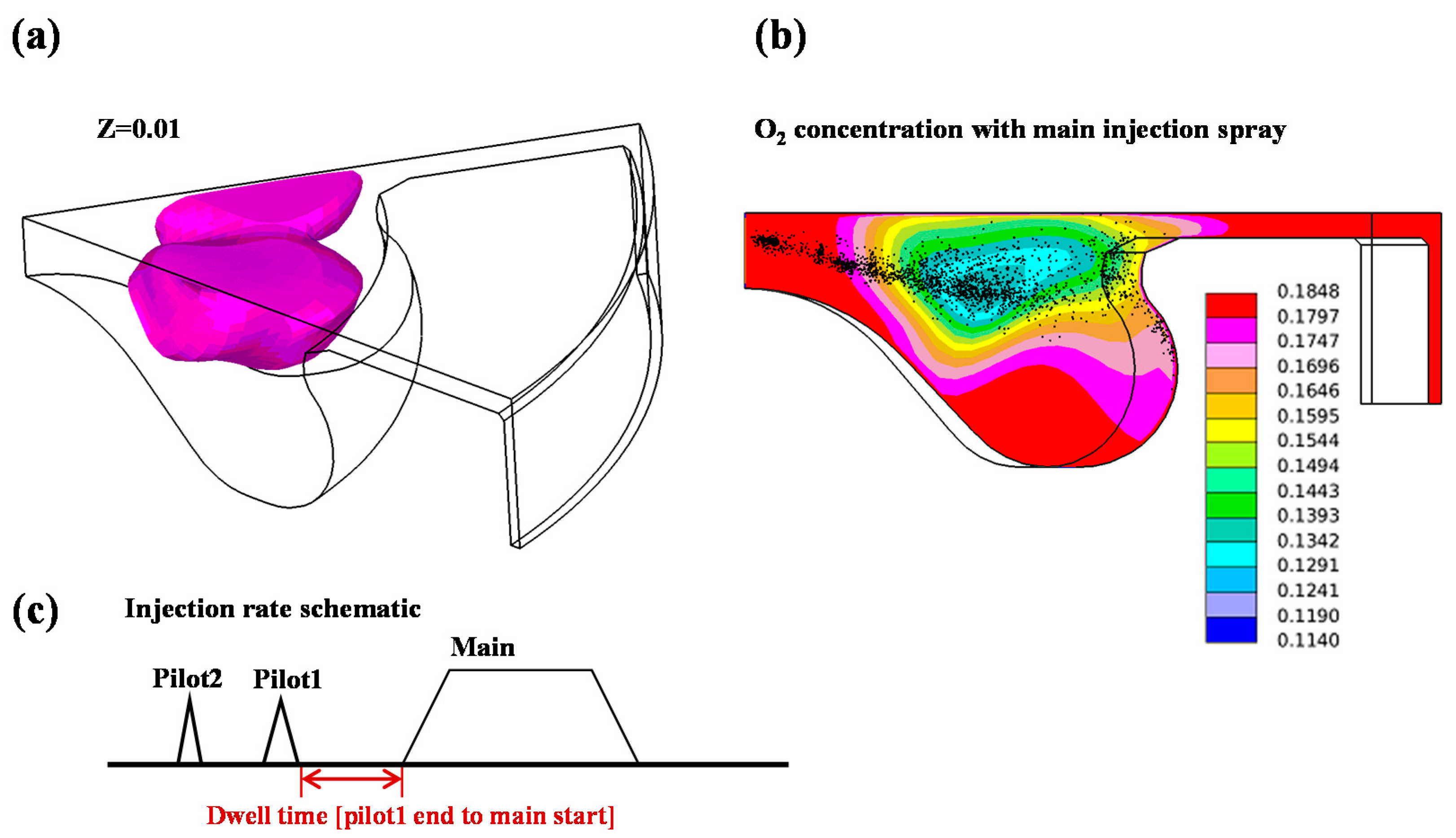
3.2.2. Determination of the NO Formation Area and Duration

In previous work [30,38], only the NO formation rate and duration were taken into account to predict the engine-out NO. However, as shown in the optical experiments [40], the high-temperature reaction area could be expanded due to the high injection pressure while the burn duration decreased. Moreover, the observation in the swirl motion revealed that the difference between the up and down sides of the jet can be varied depending on the in-cylinder conditions [40]. The given phenomenon shows that the major NO forming flame volume or area (here after treated as the surface area) can be varied and affects the formation duration. In other words, the average formation rate, as shown by Equation (18), only captures the relatively stronger or weaker formation rate at a point and does not consider a varying spatial distribution of the major NO formation area. To delineate the spatial distribution of the formation area and the duration simultaneously, the injected fuel quantity was used as a parameter. The major NO formation surface area, which is a thin layer surrounding the periphery of the fuel plume and is near a stoichiometric region, should be proportional and limited by the total injected fuel quantity because the region cannot be formed in the absence of the fuel. After adopting the parameter, the NO estimation equation can be written as:
Estimated NO  = NO   formation   at   a   point   of   flame   sheet × characteristic   area ×   duration = A T max 1 2 exp ( 69090 T max ) [ O 2 ] 1 2 [ N 2 ] ×   Fuel   quantity / engine   speed
The engine speed in Equation (19) is used as a correlation parameter for the relative change in duration that occurs from the absolute time difference.

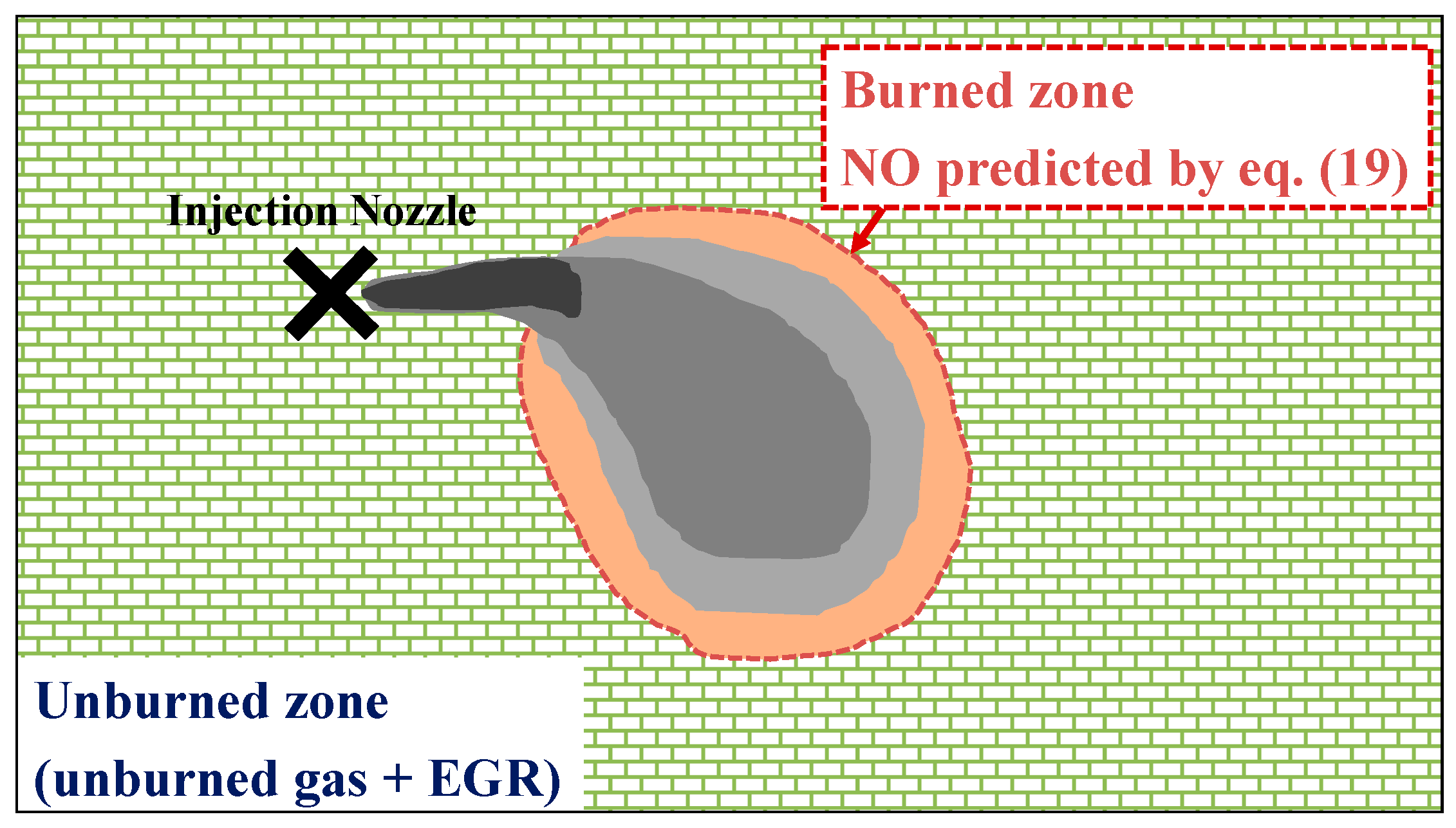
3.3. Spatial Concentration Correction of the Calculated NO

The in-cylinder area of a diesel engine can be separated into two zones because of the diffusion flame that occurs in lean circumstances. Each zone contributes to the near-diffusion flame that is directly related to the combustion and unburned zone, which consists of the unburned gas and the EGR, respectively. In Figure 5, these zones are represented by the burned and unburned zone.
The NO concentration, which is calculated using Equation (19), only considers the NO formation (mol) in the burned zone. The actual NO concentration, which is measured by the devices or tail pipe, is the NO (mol) divided by the volume of the total in-cylinder area (burned + unburned).
To correct this spatial discrepancy between the calculated and measured, a simple concentration correction factor was derived based on the ideal gas equation:
P V = m R T
where P, V, m, R and T are the pressure, volume, mass, specific gas constant and temperature, respectively. For the correction, only the volume of the unburned zone was replaced by a known value. The assumptions for the volume of the unburned substitution are as follows:
(1)
Pressure in the burned zone and the unburned zone are identical. (Pbunred = Punburned)
(2)
The mass ratio of the burned to the unburned can be expressed as the global equivalent ratio (Φ) divided by (1 − Φ).
(3)
The temperature in the burned zone (Tburned) is treated as the maximum burned gas temperature (Tmax).
(4)
The temperature in the unburned zone can be calculated using the isentropic compression and expansion relationship:
T u b _ max = T S O C × ( P max P S O C ) k 1 k
where the letters indicate the temperature in the unburned zone, the temperature of the main SOC, the maximum pressure, the pressure at SOC, and the specific heat ratio, respectively.
The equation for the engine-out NO concentration:
NO   [ mol ] V b u r n e d + V u n b u r n e d
can be re-written as follows
NO   [ mol ] V o l u m e   b u r n e d × g l o b a l   e q u i v a l e n t   r a t i o   ( ) × T max T u n b u r n e d

3.4. Fitting of the Constant in the NO Estimation Model

In a traditional approach, the NO emission predicted by the thermal NO mechanism alone is common. However, other NO mechanisms, such as from N2O or NO decomposition, cannot be neglected in some particular operating conditions (which occur, e.g., at very high rates of EGR) [14,41]. Taking into account other NO formation and decomposition mechanisms simultaneously, the final NO rate equation can be written as:
d N O d t f i n a l = d N O d t f o r m a t i o n   d N O d t d e c o m p o s i t i o n
The final rate equation described above is equal to the superposition of each NO formation rate equation and the NO decomposition rate equation. Although the complete chemical kinetic calculation from multiple mechanisms gives more accurate results, the computation time increases considerably. One way to cope with the problem is through the introduction of a correction in the previous methods to maintain the advantages of the former model [41]. Therefore, the NO formation via the N2O intermediate pathway and NO decomposition through the reverse Zeldovich and N2O mechanism were approximated by changing the rate constant of Equation (19). For use in the real-time estimation, the superposition of the exponential terms was replaced by an empirically approximation using only one exponential term. The rate constant in Equation (19), −69,090, is replaced with −33,050, which empirically approximated the value obtained using the MATLAB curve fitting function. The fitted rate constant differing from 69,090 has been observed in engine results, as in [42,43,44]. As shown by Mellor, the activation temperatures for N2O formation and the Zeldovich formation mechanism have been shown at 36,120 and 62,184 K [43]. The former value was comparable to Plee’s observation of 34,300 in a direct injection (DI) engine [44] and our tuned value of 33,050. This might lead to the conclusion that the N2O formation mechanism is dominant, but in-cylinder NO is not solely dependent on a single mechanism, and this requires additional exploration. Due to practical constraints, this paper cannot provide a comprehensive review of all NO formation and decomposition mechanisms. The final form of the NO prediction equation can be expressed as:
Estimated NO  [ ppm ] = NO   formation   at   a   point   of   flame   sheet   ( empirically   fitted ) × characteristic   area ×   duration   × spatial   concentration   correcttion = A T max 1 2 exp ( 33050 T max ) [ O 2 ] 1 2 [ N 2 ] ×   Fuel   quantity / RPM × × T max T u n b u r n e d
The NO prediction results using Equation (25) are shown in the results and discussion section.

4. Results and Discussion

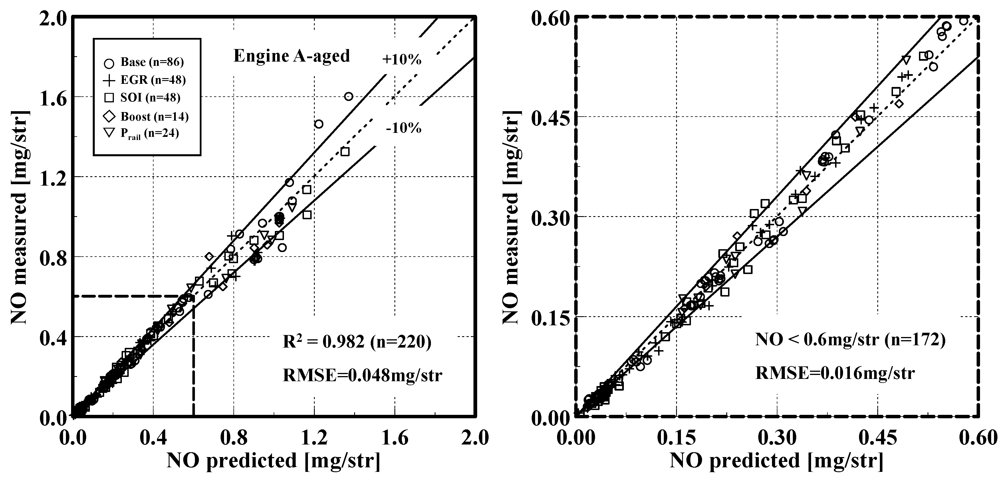
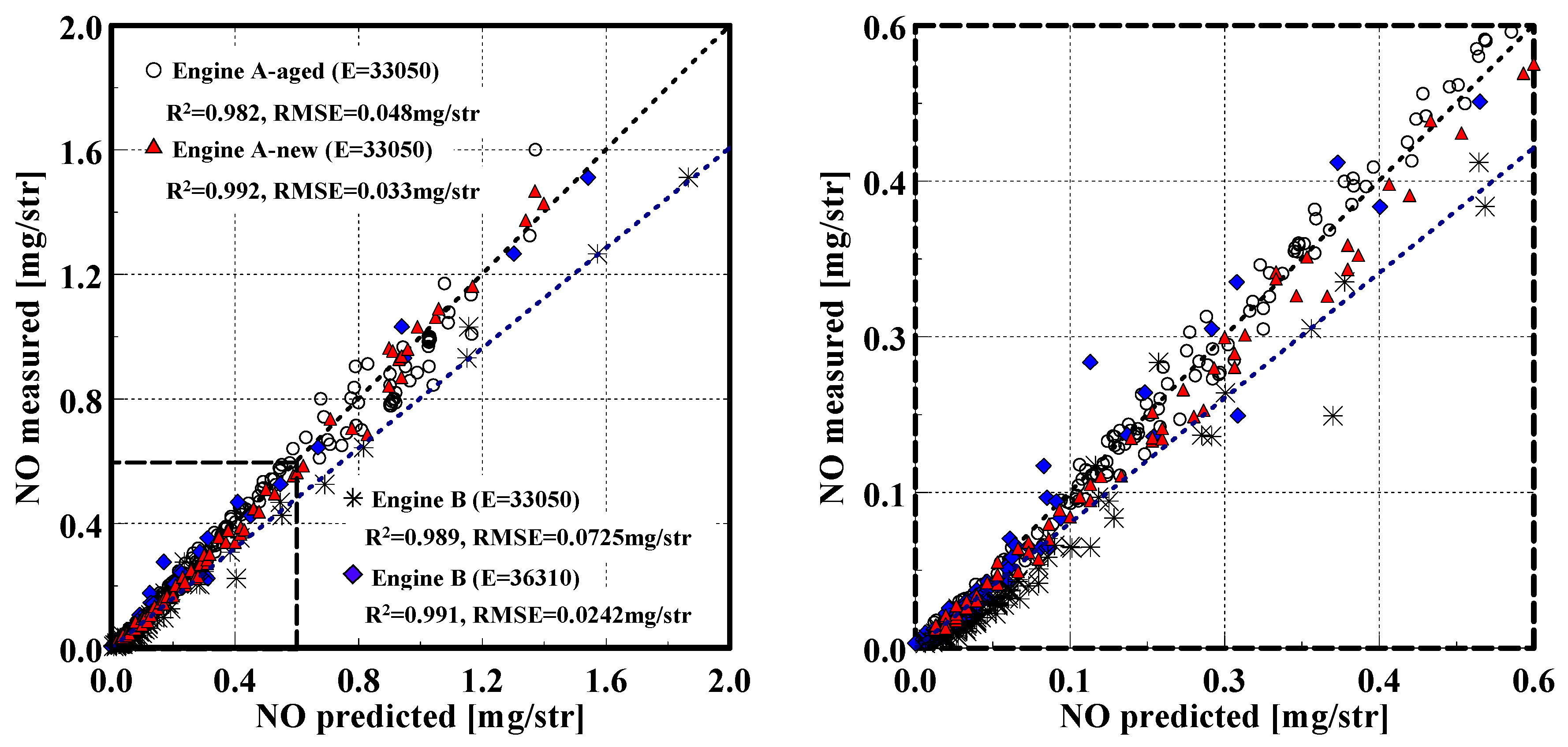
4.1. Model Application in Steady-State Operation Conditions

The NO estimation model in Equation (25) was applied to the steady-state operating condition that is presented in Table 3. To validate the model’s potential, the cylinder charge-related parameters, which are the EGR, the boost pressure and injection-related parameters, the rail pressure, and the injection timing, were swept compared to nominal operating points. Figure 6 reports the estimated engine-out NO emission with respect to the measured NO emission. The correlation coefficient R2 and the RMSE are shown to quantitatively analyze the model accuracy. The R2 value of 0.982 and the RMSE value of 0.048 (mg/str) are noted as giving good predictability. The model was found to have errors of approximately ±10% compared to the measured NO, although there are greater errors at some points. Moreover, there was nothing particularly remarkable in the NO estimation results while parameters, such as the EGR, SOI, boost pressure and the rail pressure, were changed.

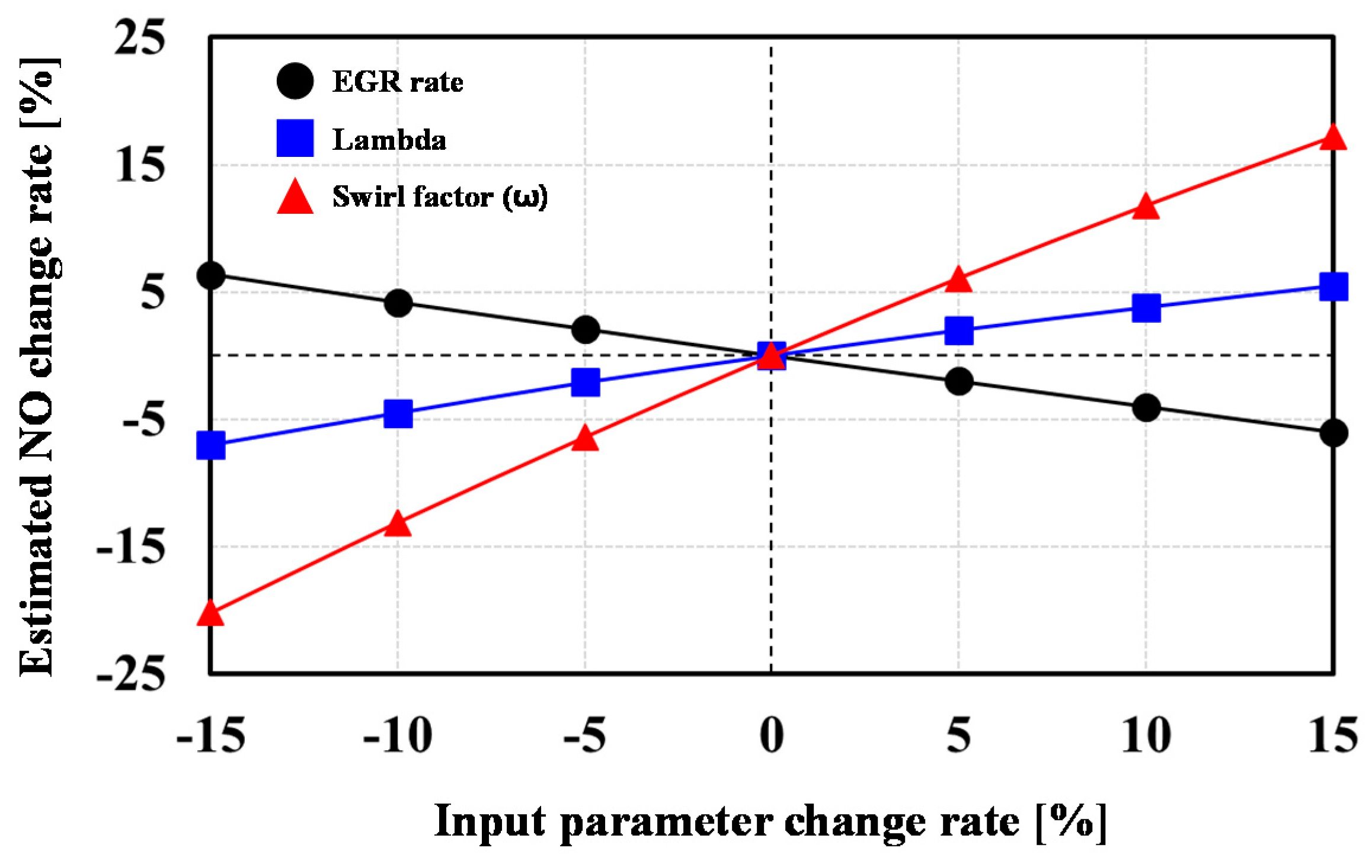
4.2. Evaluation of the Model Input Parameter Sensitivity Analysis

To examine errors in the measurement and calculation, a sensitivity analysis was performed with the EGR, lambda, and the swirl factor using the proposed NO estimation model. The reason for selecting these parameters was to precisely investigate the impact of the measurement uncertainty from the ECU. Moreover, the EGR is known to be a dominant factor in NO production from CI engines because, through the use of the EGR, the combustion temperature decreases due to a lower oxygen concentration and a greater heat capacity compared to when fresh air is supplied. Similarly, lambda and the swirl factor (ω) are indicators of the in-cylinder oxygen concentration; specifically, the swirl factor represents burned gas of pilot fuel mixing before the main event.
In Figure 7, the errors in the calculation come from the EGR rate, and other inputs such as lambda and the swirl factor are shown. The results were derived by offsetting the parameters from all operating points in engine A-aged (n = 220). The sensitivity analysis of the EGR rate on the NO estimation showed that a 15% offset in the EGR rate can cause a nearly 5% error in the NO estimation. Changing lambda by 15% resulted in similar results as the EGR rate adjustment, which is expected because both parameters are used in Equation (2). Although the influences were analogous, the changing trend was opposite because they affect the cylinder temperature in opposite manners. An important conclusion of this analysis is that variables with more influence on estimating the NO emissions are the swirl factor (ω), which depends on the swirl ratio, the dwell time, and the engine speed, as described in Section 3.1. The results indicate that the pilot burned gas distribution and the mixing are very sensitive in our estimation model while the remainder of the parameters have less influence.

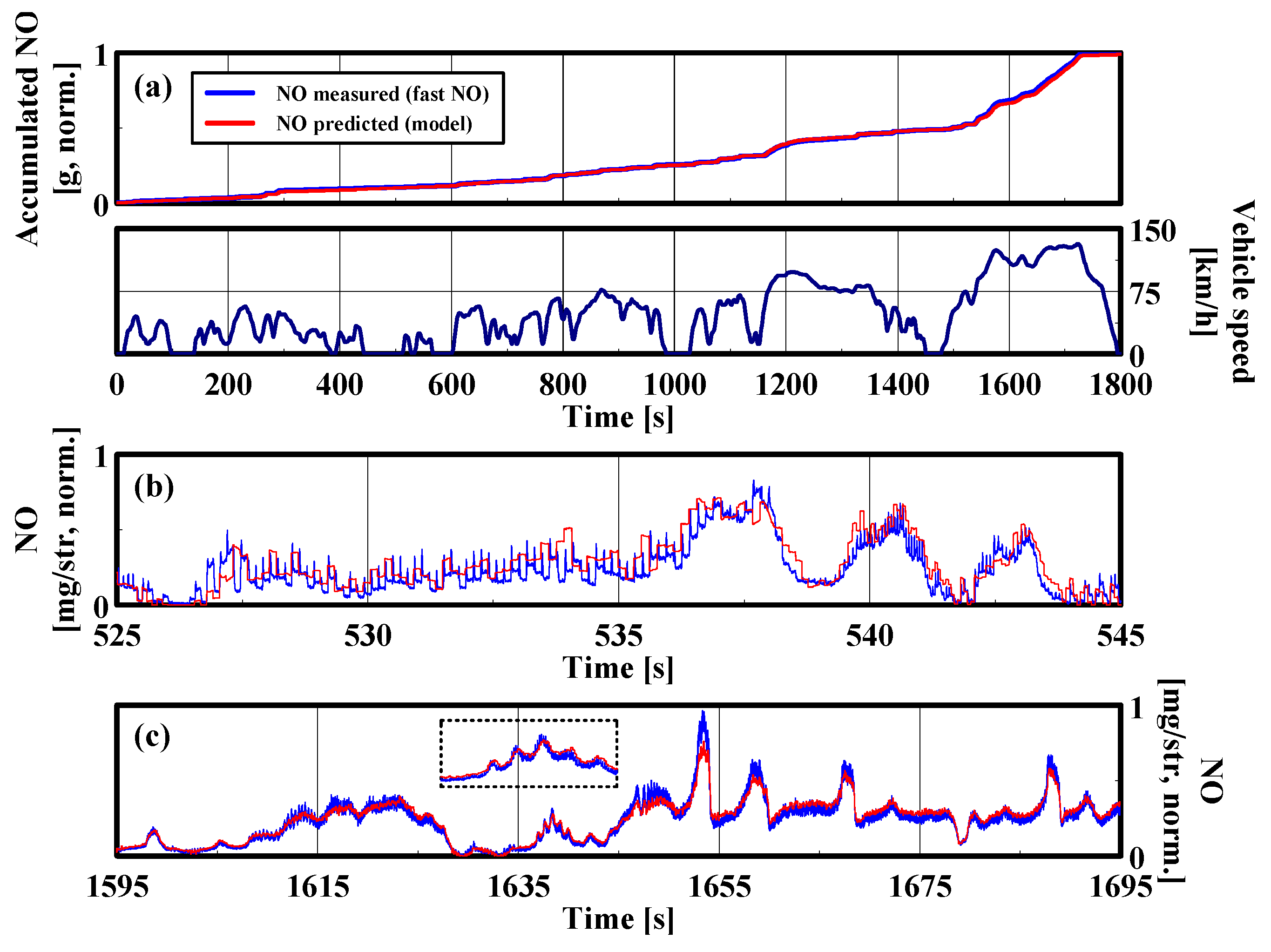
4.3. Model Application in Transient Operation Conditions over a WLTC

The performance of the proposed model was evaluated in transient conditions, and these conditions are referred to as WLTC. The WLTC is separated into four phases (low, medium, high, extra-high), and the real-time estimation results show portions of the low and extra-high phases, as seen in Figure 8. The airflow rate and the injected fuel quantity delivered from the ECU were used to calculate the total NO mass, and from this calculation, the NO accumulation curve with respect to the time history was obtained. Figure 8a shows the cumulative NO mass emission over the entire WLTC.
The cumulative emissions were normalized with respect to the Mexa-7100-measured value for comparison. As shown in the graph, the accumulation of the estimated NO almost matched the measured NO over the entire time history, and the final errors are within 1.5%. The vehicle velocity profiles for the WLTC are aligned with the NO accumulation results. The magnified information was selected based on the lower and higher part of the vehicle velocity, and these areas corresponds with the low and extra-high phases in the WLTC, respectively. Twenty seconds of the low phase, which expressed the NO variation well, is shown in Figure 8b. This timescale allows the assessment of cyclic variations in the NO measurement and estimation. The mass of the NO emission in the timescale was normalized and is shown in the window.
In the first part of the graph, a regular peak wave from the measured data clearly shows the exhaust stroke, and the square wave from the model obviously shows the capability of the real-time, cycle-by-cycle NO estimation. Note that to observe individual cycle events, a fast NO analyzer probe was mounted near the exhaust valve, while the model input AF was from an engine mounted sensor located beyond the turbocharger. It is possible that the delay when the NO changes rapidly or the absolute level difference between the estimated and measured results from the fast NO analyzer could have been caused by exhaust gas mixing in the cylinders beyond the turbocharger [45] or due to AF sensor delay compared to the fast-response analyzer. Figure 8c shows that the normalized NO mass from 1595 s to 1695 s had greater model predictability during significant NO transient conditions. Additionally, this result is presented in the insert within the graph, which enlarges the time period from 1635 s to 1640 s.

4.4. Model Robustness Validation

In this section, the main focus is to verify the model robustness in diverse ways. The model was applied to engine A-aged and engine A-new to identify the difference in not only the hardware (e.g., the injector, EGR system, and turbocharger) age but also the hardware difference between the conventional series production because engine A was entirely changed. Moreover, engine-B, which is totally different from engine A (detailed in the experimental section), was used to assure the model’s capability. The NO prediction in engine-B was conducted using two methods: one using the same calibration constant as engine-A and one in which the constant was recalibrated for engine B. In Figure 9, the predicted versus the measured NO in the three engines with many different operating conditions is presented. A good agreement for engine A-aged was observed, as shown in Section 4.1, and a good trend was observed when the NO estimation model was applied to engine A-new. There was a slight increase in the correlation coefficient R2: 0.992, and there was an improvement in the RMSE: 0.033 mg/str. This change possibly came from the experimental set differences, as noted in Table 3.
In addition, the NO estimation results from engine B with a calibration constant identical to the one applied to engine A-aged and A-new still shows a good correlation value R2 of 0.989, although the RMSE value increased compared to the predicted results of engine A (Note that ω in Equation (12) re-scaled in the same manner using the maximum values used in the engine B experimental conditions). The increase in the RMSE value comes from the overestimated results compared to the measured value, as shown by the decreasing trend line in Figure 9. However, the behavior of the model is, in general, quite robust even though the model was not been recalibrated for engine B. The recalibration of the model constants for engine B enhanced the predictability with a R2 of 0.991 and an RMSE of 0.0242 mg/str. The estimated NO in engine B with the adjusted constant (E = 36,310 in Equation (25)) lined closely with the diagonal of the results from engine A, which leads to the RMSE improvement.
After confirming the model robustness using different hardware at steady operation circumstances, the model’s capability was verified in the WLTC where external perturbations existed. The selected artificial perturbations offset the intake air mass flow rate map, which is built in ECU as a function of the operating points and bypasses the exhaust gas prior to the turbocharger. The intake airflow rate map was offset to mimic drift or to weaken the sensitivity of the inherent sensors, such as the airflow, or boost pressure that might be caused by aging. Table 4 shows the cumulative NO mass emissions over the WLTC with general and ±3% entire air map offset conditions. The 3% deviation in the airflow rate map cause a nearly 10% deviation in the NO accumulation during the cycle due to EGR rate change. The EGR rate was increased when the negative offset was applied and was decreased when the positive offset was applied due to in-cylinder fresh air mass change. The EGR rate deviated by a maximum of 9% compared with general transient operation when the air map changed ±3%, respectively. Regardless of the variation, the estimated mass of NO was within 3% of the measured value during the WLTC.
Moreover, the exhaust gas prior to the turbocharger was bypassed to create a hardware malfunction in the air charging system specifically. Bypassing the turbocharger boosted the pressure decrease because the turbocharger operated outside of the designed region, although the target value was identical, and consequently, there was relatively reduced intake manifold pressure, which allows for a greater portion of the EGR to flow in the manifold. Finally, the rose of the EGR rate increased the global in-cylinder global equivalent ratio significantly when the injection fuel amount and timing were equal. The selected deviations for the general and bypassed conditions are noted in Table 5.
As shown in Table 4, a significant reduction in the cumulative NO emission was observed when the exhaust gas bypassed the turbocharger. The explanation for the nearly 26% cumulative NO mass decrease in the cycle was the reduced in-cylinder fresh air mass of the air system. However, the estimated cumulative NO mass demonstrated meaningful results with the measured value in this unfavorable condition. Accordingly, from this diverse approach, the proposed NO prediction model is quite reliable during both aging and hardware malfunctions.

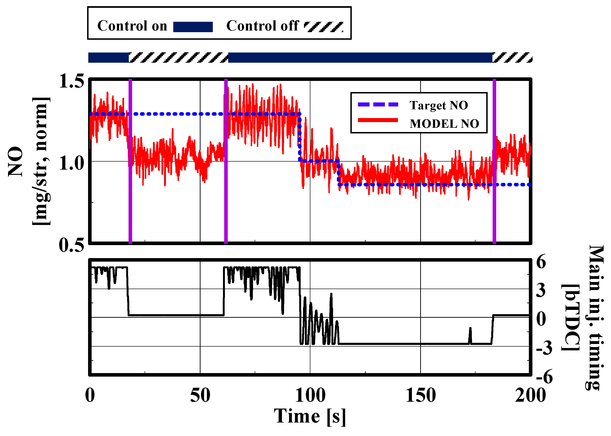
4.5. Real-Time NO Emission Control during Steady-State Operating Conditions

Finally, the model was applied to a real-time engine-out NO emission control during steady-state operation. The injection timing for the main was selected as a control parameter because of the immediate emission responsibility and was adjusted to change the engine-out NO. The main injection timing was controlled using a closed-control scheme that compared the NO estimation value to a target value. The procedure for the real-time engine-out NO emission control process is shown in Figure 10.
The control logic was turned on and off alternatively for 200 s to examine the NO control capability. As reported in Figure 10, the main injection timing varied within the range of bTDC −3 to 5 CA to maintain engine stability, and the range of NO emissions were normalized with the NO level. The engine-out NO instantaneously varied when the control logic was applied, and the change was from −10% to 30% compared to the nominal condition. The main injection timing was saturated to the lower boundary value between 110 and 180 s due to the limitation of the timing, and this caused a slight deviation with the target value. However, nearly 40% of the raw emission can be varied successfully with the NO estimation model used in the real-time NO emission control.

5. Conclusions

The present work introduces a physics-based, computationally applicable NO estimation model that is capable of cycle-by-cycle engine-out NO emission determination. The objective of the proposed research was to use physical concepts with simplification to develop an on-ECU NO estimator. To achieve this goal, the model utilized the in-cylinder pressure and the data available from the ECU.
The model considers the maximum burned gas temperature of the main injection and takes into account the pilot fuel burning and mixing. From the calculated temperature, the averaged NO formation rate was determined. In addition, the NO formation area change that accompanies the formation duration variation was treated proportionally to the injected fuel quantity for simplification. After calculating the formation rate, area, and duration, a spatial correction for the NO formation due to the heterogeneous reaction was compensated for using a simple correlation.
As shown in the paper, the proposed model is capable of taking into account the injection timing, the rail pressure, the boost pressure and the EGR rate variations on the NO emissions. Based on the agreement over an extensive range of steady-state conditions (R2: 0.98, RMSE: 0.048 mg/str), the model was validated using the WLTC (accumulation error within 3%). The cycle-by-cycle prediction capability in the WLTC demonstrates that the computational cost was satisfactorily low, and due to the fast calculation, the engine-out NO emission was controlled by changing the main injection timing. The model robustness was demonstrated with three engines and on two different types of engines that were representative of light-duty vehicles. The proposed virtual NO sensor can be a useful tool as follows:
(1)
as an engine emission calibrator in the engine development stage
(2)
for the real-time management of exhaust NO emissions
(3)
as an alerting system for physical NOx sensor failure

Acknowledgments

The authors would like to thank the advanced diesel engine development team at the Hyundai Motor Group for their technical support. This research was supported by the Hyundai Motor Group and the Seoul national university institute of advanced machines and design (SNU IAMD).

Author Contributions

Seungha Lee and Kyoungdoug Min conceived and designed the experiments; Seungha Lee and Youngbok Lee performed the experiments; Seungha Lee, Youngbok Lee and Gyujin Kim analyzed the data; Gyujin Kim contributed analysis tools; Seungha Lee and Kyoungdoug Min wrote the paper.

Conflicts of Interest

The authors declare no conflict of interest.

Abbreviations

Aa constant in Equation (18)
aa constant in Equation (2)
A/Danalog/digital
AFair-fuel ratio
aTDCafter top dead center
ba constant in Equation (2)
bTDCbefore top dead center
BMEPBrake Mean Effective Pressure (bar)
ca constant in Equation (2)
CACrank Angle (degree)
COcarbon monoxide
CO2carbon dioxide
CRDIcommon rail direct injection
da constant in Equation (2)
DPFDiesel Particulate Filter
DTDwell Time (time interval between the end of pilot1 injection and start of main injection, s)
ECUEngine Control Unit
EGRExhaust Gas Recirculation (-)
EMS Engine Management System
EVCexhaust valve close
EVOexhaust valve open
IVCintake valve close
IVOintake valve open
kspecific heat ratio
LNTLean NOx Trap
RMSERoot mean square error (mg/str)
ROHRRate of Heat Release
Mmass (kg)
NOnitric monoxide
NO2nitrogen dioxide
NOxnitric oxides
Ppressure (bar)
SCRselective catalytic reduction
SVOSwirl Valve Opening (%)
Ttemeperature (K)
Vvolume (m3)
VGTvariable geometry turbine
WLTCworldwide harmonized light vehicles test cycle
Zmixture fraction (-)
Greek Symbols
αair availability (-)
δa constant in Equation (11) (-)
λair-excess ratio (-)
ψmolar N/O ratio (-)
ΦEquivalence ratio (-)
ωSwirl factor (-)
Subscripts
adadiabatic
eequilibrium concentration
maxmaximum
SOCstart of combustion
ubunburned

References

  1. Mauzerall, D.L.; Sultan, B.; Kim, N.; Bradford, D.F. NOx emissions from large point sources: Variability in ozone production, resulting health damages and economic costs. Atmos. Environ. 2005, 39, 2851–2866. [Google Scholar] [CrossRef]
  2. Meszler, D.; German, J.; Mock, P.; Bandivadekar, A. CO2 Reduction Technologies for the European Car and Van Fleet, A 2025–2030 Assessment; The International Council on Clean Transportation (ICCT): Berlin, Germany, 2016. [Google Scholar]
  3. Yang, Z. Improving the Conversions between the Various Passenger Vehicle Fuel Economy/CO2 Emission Standards Around the World; The International Council on Clean Transportation (ICCT): Berlin, Germany, 2014. [Google Scholar]
  4. Sarangi, A.K.; McTaggart-Cowan, G.P.; Garner, C.P. The Effects of Intake Pressure on High EGR Low Temperature Diesel Engine Combustion; 0148-7191, SAE Technical Paper; SAE International: Warrendale, PA, USA, 2010. [Google Scholar]
  5. Kimura, S.; Aoki, O.; Kitahara, Y.; Aiyoshizawa, E. Ultra-Clean Combustion Technology Combining a Low-Temperature and Premixed Combustion Concept for Meeting Future Emission Standards; SAE Technical Paper; SAE International: Warrendale, PA, USA, 2001. [Google Scholar]
  6. Colban, W.F.; Miles, P.C.; Oh, S. Effect of Intake Pressure on Performance and Emissions in an Automotive Diesel Engine Operating in Low Temperature Combustion Regimes; SAE Technical Paper; SAE International: Warrendale, PA, USA, 2007. [Google Scholar]
  7. Alriksson, M.; Denbratt, I. Low Temperature Combustion in a Heavy Duty Diesel Engine Using High Levels of EGR; 0148-7191, SAE Technical Paper; SAE International: Warrendale, PA, USA, 2006. [Google Scholar]
  8. Forzatti, P.; Lietti, L.; Nova, I.; Tronconi, E. Diesel Nox aftertreatment catalytic technologies: Analogies in lnt and scr catalytic chemistry. Catal. Today 2010, 151, 202–211. [Google Scholar] [CrossRef]
  9. Theis, J.; Gulari, E. A LNT + SCR System for Treating the NOx Emissions from a Diesel Engine; 0148-7191, SAE Technical Paper; SAE International: Warrendale, PA, USA, 2006. [Google Scholar]
  10. Curran, S.; Hanson, R.; Wagner, R.; Reitz, R.D. Efficiency and Emissions Mapping of RCCI in a Light-Duty Diesel Engine; 0148-7191, SAE Technical Paper; SAE International: Warrendale, PA, USA, 2013. [Google Scholar]
  11. Kihas, D.; Uchanski, M.R. Engine-Out NOx Models for On-Ecu Implementation: A Brief Overview; 0148-7191, SAE Technical Paper; SAE International: Warrendale, PA, USA, 2015. [Google Scholar]
  12. D’Ambrosio, S.; Finesso, R.; Fu, L.; Mittica, A.; Spessa, E. A control-oriented real-time semi-empirical model for the prediction of NOx emissions in diesel engines. Appl. Energy 2014, 130, 265–279. [Google Scholar] [CrossRef]
  13. Asprion, J.; Chinellato, O.; Guzzella, L. A fast and accurate physics-based model for the Nox emissions of diesel engines. Appl. Energy 2013, 103, 221–233. [Google Scholar] [CrossRef]
  14. Andersson, M.; Johansson, B.; Hultqvist, A.; Noehre, C. A predictive Real Time NOx Model for Conventional and Partially Premixed Diesel Combustion; 01-3329, SAE Technical Paper; SAE International: Warrendale, PA, USA, 2006. [Google Scholar]
  15. Egnell, R. Combustion diagnostics by means of multizone heat release analysis and No calculation. SAE Trans. J. Engines 1998, 107. [Google Scholar] [CrossRef]
  16. Del Re, L.; Allgöwer, F.; Glielmo, L.; Guardiola, C.; Kolmanovsky, I. Automotive Model Predictive Control: Models, Methods and Applications; Springer: Berlin, Germany, 2010. [Google Scholar]
  17. Arrègle, J.; López, J.J.; Guardiola, C.; Monin, C. Sensitivity Study of a NOx Estimation Model for On-Board Applications; 0148-7191, SAE Technical Paper; SAE International: Warrendale, PA, USA, 2008. [Google Scholar]
  18. Seykens, X.; Baert, R.; Somers, L.; Willems, F. Experimental validation of extended no and soot model for advanced hd diesel engine combustion. SAE Int. J. Engines 2009, 2, 606–619. [Google Scholar] [CrossRef]
  19. Willems, F.; Doosje, E.; Engels, F.; Seykens, X. Cylinder Pressure-Based Control in Heavy-Duty EGR Diesel Engines Using a Virtual Heat Release and Emission Sensor; SAE Paper; SAE International: Warrendale, PA, USA, 2010. [Google Scholar]
  20. Hegarty, K.; Favrot, R.; Rollett, D.; Rindone, G. Semi-Empiric Model Based Approach for Dynamic Prediction of NOx Engine Out Emissions on Diesel Engines; 0148-7191, SAE Technical Paper; SAE International: Warrendale, PA, USA, 2010. [Google Scholar]
  21. Finesso, R.; Spessa, E. Real-Time Predictive Modeling of Combustion and Nox Formation in Diesel Engines under Transient Conditions; 0148-7191, SAE Technical Paper; SAE International: Warrendale, PA, USA, 2012. [Google Scholar]
  22. Eriksson, L.; Nielsen, L. Modeling and Control of Engines and Drivelines; John Wiley & Sons: New York, NY, USA, 2014. [Google Scholar]
  23. Schejbal, M.; Štěpánek, J.; Marek, M.; Kočí, P.; Kubíček, M. Modelling of soot oxidation by NO2 in various types of diesel particulate filters. Fuel 2010, 89, 2365–2375. [Google Scholar] [CrossRef]
  24. Zhang, Z.-S.; Crocker, M.; Chen, B.-B.; Wang, X.-K.; Bai, Z.-F.; Shi, C. Non-thermal plasma-assisted Nox storage and reduction over cobalt-containing lnt catalysts. Catal. Today 2015, 258, 386–395. [Google Scholar] [CrossRef]
  25. Iwasaki, M.; Shinjoh, H. A comparative study of “standard”,“fast” and “NO2” scr reactions over fe/zeolite catalyst. Appl. Catal. A Gen. 2010, 390, 71–77. [Google Scholar] [CrossRef]
  26. Heywood, J.B. Internal Combustion Engine Fundamentals; McGraw-Hill: New York, NY, USA, 1988. [Google Scholar]
  27. Finesso, R.; Misul, D.; Spessa, E. Estimation of the Engine-Out NO2/NOx Ratio in a Euro vi Diesel Engine; 0148-7191, SAE Technical Paper; SAE International: Warrendale, PA, USA, 2013. [Google Scholar]
  28. Hernandez, J.; Lapuerta, M.; Perez-Collado, J. A combustion kinetic model for estimating diesel engine Nox emissions. Combust. Theory Model. 2006, 10, 639–657. [Google Scholar] [CrossRef]
  29. Liu, S.; Li, H.; Liew, C.; Gatts, T.; Wayne, S.; Shade, B.; Clark, N. An experimental investigation of NO2 emission characteristics of a heavy-duty h 2-diesel dual fuel engine. Int. J. Hydrog. Energy 2011, 36, 12015–12024. [Google Scholar] [CrossRef]
  30. Lee, J.; Lee, S.; Park, W.; Min, K.; Song, H.H.; Choi, H.; Yu, J.; Cho, S.H. The Development of Real-Time NOx Estimation Model and Its Application; 0148-7191, SAE Technical Paper; SAE International: Warrendale, PA, USA, 2013. [Google Scholar]
  31. ISO/IEC Guide 98-3:2008. Guide to the Expression of Uncertainty in Measurement, ISO: Geneva, Switzerland, 1995.
  32. Seykens, X.L.J. Development and Validation of a Phenomenological Diesel Engine Combustion Model. Ph.D. Thesis, Eindhoven University of Technology, Eindhoven, The Netherlands, 2010. [Google Scholar]
  33. Turns, S. An Introduction to Combustion: Concepts and Applications; SAE International: Warrendale, PA, USA, 1996. [Google Scholar]
  34. Minami, T.; Takeuchi, K.; Shimazaki, N. Reduction of Diesel Engine NOx Using Pilot Injection; 0148-7191, SAE Technical Paper; SAE International: Warrendale, PA, USA, 1995. [Google Scholar]
  35. Colin, O.; Benkenida, A. The 3-zones extended coherent flame model (ecfm3z) for computing premixed/diffusion combustion. Oil Gas Sci. Technol. 2004, 59, 593–609. [Google Scholar] [CrossRef]
  36. Kim, G.; Min, K. Numerical Study on the Multiple Injection Strategy in Diesel Engines Using a Modified 2-d Flamelet Model; 0148-7191, SAE Technical Paper; SAE International: Warrendale, PA, USA, 2015. [Google Scholar]
  37. Peters, N. Turbulent Combustion; Cambridge University Press: Cambridge, UK, 2000. [Google Scholar]
  38. Park, W.; Lee, J.; Min, K.; Yu, J.; Park, S.; Cho, S. Prediction of real-time no based on the in-cylinder pressure in diesel engines. Proc. Combus. Inst. 2013, 34, 3075–3082. [Google Scholar] [CrossRef]
  39. Finesso, R.; Spessa, E. Ignition delay prediction of multiple injections in diesel engines. Fuel 2014, 119, 170–190. [Google Scholar] [CrossRef]
  40. Le, M.K.; Kook, S. Injection pressure effects on the flame development in a light-duty optical diesel engine. SAE Int. J. Engines 2015, 8, 609–624. [Google Scholar] [CrossRef]
  41. Arrègle, J.; López, J.J.; Guardiola, C.; Monin, C. On board NOx prediction in diesel engines: A physical approach. In Automotive Model Predictive Control; Springer: Berlin, Gemany, 2010. [Google Scholar]
  42. Guardiola, C.; López, J.J.; Martín, J.; García-Sarmiento, D. Semiempirical in-cylinder pressure based model for NOx prediction oriented to control applications. Appl. Therm. Eng. 2011, 31, 3275–3286. [Google Scholar] [CrossRef]
  43. Mellor, A.M.; Mello, J.; Duffy, K.P.; Easley, W.; Faulkner, J. Skeletal Mechanism for NOx Chemistry in Diesel Engines; SAE Technical Paper; SAE International: Warrendale, PA, USA, 1998. [Google Scholar]
  44. Plee, S.; Ahmad, T.; Myers, J.; Siegla, D. Effects of flame temperature and air-fuel mixing on emission of particulate carbon from a divided-chamber diesel engine. In Particulate Carbon; Springer: Berlin, Gemany, 1981. [Google Scholar]
  45. Peckham, M.; Campbell, B.; Finch, A. Measurement of the effects of the exhaust gas recirculation delay on the nitrogen oxide emissions within a turbocharged passenger car diesel engine. J. Automob. Eng. 2011, 225, 1156–1166. [Google Scholar] [CrossRef]
Figure 1. (a) Schematic overview of the experimental setup; (b) NO calculation procedure in a cycle (solid arrows) with the control process (dotted arrows).
Energies 10 00284 g001
Figure 2. Experimental conditions for steady-state evaluation. Clusters of marks are shown when operating parameters were swept. The engine speed test conditions were equivalent to engine A-new (n = 91), but engine A-aged (n = 220) and engine B (n = 99) are shifted aside for visibility.
Energies 10 00284 g002
Figure 3. Structure of the real-time NO estimation model (The patterned arrows represent the data from the ECU and the blanked arrows indicate the data from the in-cylinder pressure. The solid arrows show the on-board calculation processes).
Energies 10 00284 g003
Figure 4. The CFD simulations at 6 aTDC CA showing (a) the mixture fraction contours at Z = 0.01; (b) the O2 mole fraction with the main injection spray. The reference condition was 1500 rpm, pilot2 1.1/pilot1 1.35 mg/str, DT 7.24CA, main injection timing at 0.7 bTDC CA; and (c) Injection rate schematic. (bTDC means before top dead center)
Energies 10 00284 g004
Figure 5. Schematic of the in-cylinder burned and unburned zone.
Energies 10 00284 g005
Figure 6. Steady-state NO estimated using the model compared to measured values in engine A-aged. All operating points with parameter variations (n = 220) and a magnification of relatively small ranges (NO < 0.6 mg/str) are shown.
Energies 10 00284 g006
Figure 7. Results of the sensitivity analysis for all operating points in engine A-aged (n = 220).
Energies 10 00284 g007
Figure 8. (a) The normalized cumulative mass of the NO and the velocity profile of the WLTC with respect to time; (b) Magnified time window to show the cycle-by-cycle estimated and measured real-time NO emissions in a portion of the WLTC (low phase); (c) Estimated and measured NO emissions mass vs. time history (extra-high phase), (red: model predicted, blue: fast NO analyzer measured).
Energies 10 00284 g008
Figure 9. Steady-state NO mass of estimated using the model compared to the measured values in engine A-aged (n = 220, ○), engine A-new (n = 91, △), engine B (n = 99, *) with the same constant (E = 33,050) as engine-A, and engine B (n = 99, ◇) with the constant (E = 36,310) recalibrated, and an enlargement of a relatively small range (NO < 0.6 mg/str) of the estimation results are shown.
Energies 10 00284 g009
Figure 10. Engine-out NO emission control during steady-state conditions (1500 rpm, 25 mg/str).
Energies 10 00284 g010
Table 1. Key specifications of the test engines.
Engine TypeIn-Lined Compression Ignition 4 Cylinders
EURO5 (Engine A)EURO6 (Engine B)
Displaced volume1582 cc2199 cc
Bore × Stroke77.2 mm × 84.5 mm85.4 mm × 96 mm
Compression ratio17.316
Turbocharger typeSingle stage VGTSingle stage E-VGT
Fuel injection systemCRDI (Solenoid injector)CRDI (Solenoid injector)
Maximum power and torque94 kW/260 N.m150 kW/440 N.m
Valve timingIVO/IVC (ATDC17/ABDC14)
EVO/EVC (BBDC23/BTDC 20)
IVO/IVC (ATDC10/ABDC7)
EVO/EVC (BBDC32/BTDC17)
Table 2. Main sources of measurement errors and the expanded uncertainties.
DeviceErrorExpanded Uncertainty (%)
Fast NO analyzerZero drift<5 ppm/h≤2.1
Span drift<1% full scale/h
Exhaust gas analyzerZero drift<1% full scale/24 h≤4.5
Span drift<1% full scale/24 h
Noise<2% full scale
Linearity<1% full scale
Piezo electric sensorLinearity<0.3% full scale≤5.7
Sensitivity shift<2% (at 23–350 °C)
<0.5% (at 200 ± 50 °C)
Short term drift
(Thermal shock)
<2% for minimum pressure (9 bar)
<1% for maximum pressure (250 bar)
Charge amplifier ≤0.2
Analog/digital errorA/D conversion linearity ≤0.024
Table 3. Typical engine operating range for steady-state conditions and the sweep interval for each parameter (aTDC means after top dead center).
Experimental ConditionsEngine AEngine BSweep Interval (Based on Typical)
EGR (%)0 to 400 to 565 Steps between min/max
Minimum: −10%
Maximum: 20%
Rail pressure (bar)300 to 1400±100
Boost pressure (bar)1 to 2.3±0.1
Main injection timing (aTDC)−6 to 2±2, 4
Equivalence ratio (Φ)0.2 to 0.9
Injection per cycle3 (pilot2, pilot1, main) or 4 (pilot2, pilot1, main, post)
Pilot + Pre injection (mg/str)1 to 3
Table 4. Accumulation of the engine-out NO mass results during WLTC when artificial perturbations were applied entire intake air map offset and exhaust gas bypassed prior to the turbocharger. Note that the values were normalized with the measured value of the accumulated NO during nominal operation conditions.
Engine A-AgedMeasuredEstimatedError (%)
Air map offset−3%general+3%−3%general+3%−3%general+3%
Total NO (g, norm.)0.9041.0001.1230.8830.9851.095−2.3−1.5−2.5
Total NO_bypassed (g, norm.) 0.738 0.698 −5.4
Table 5. Major engine operating parameter changes in the selected general vs. the bypassed operating conditions. The injection strategy used was identical in for conditions (∆: based on nominal value).
Engine SpeedBMEP_General (bar)BMEP_Bypassed (bar)∆ Boost Pressure (hPa)EGR (%)φ (-)
15009.47.0−141.916.90.31
150011.48.6−138.116.80.29
20006.95.2−71.915.10.27
20009.56.8−112.415.80.32
200012.18.4−116.815.40.33
200014.410.6−80.617.00.32

