Decoupling Weather Influence from User Habits for an Optimal Electric Load Forecast System


Abstract
:1. Introduction
- the importance of an accurate forecast of photovoltaic output for low-voltage load estimation;
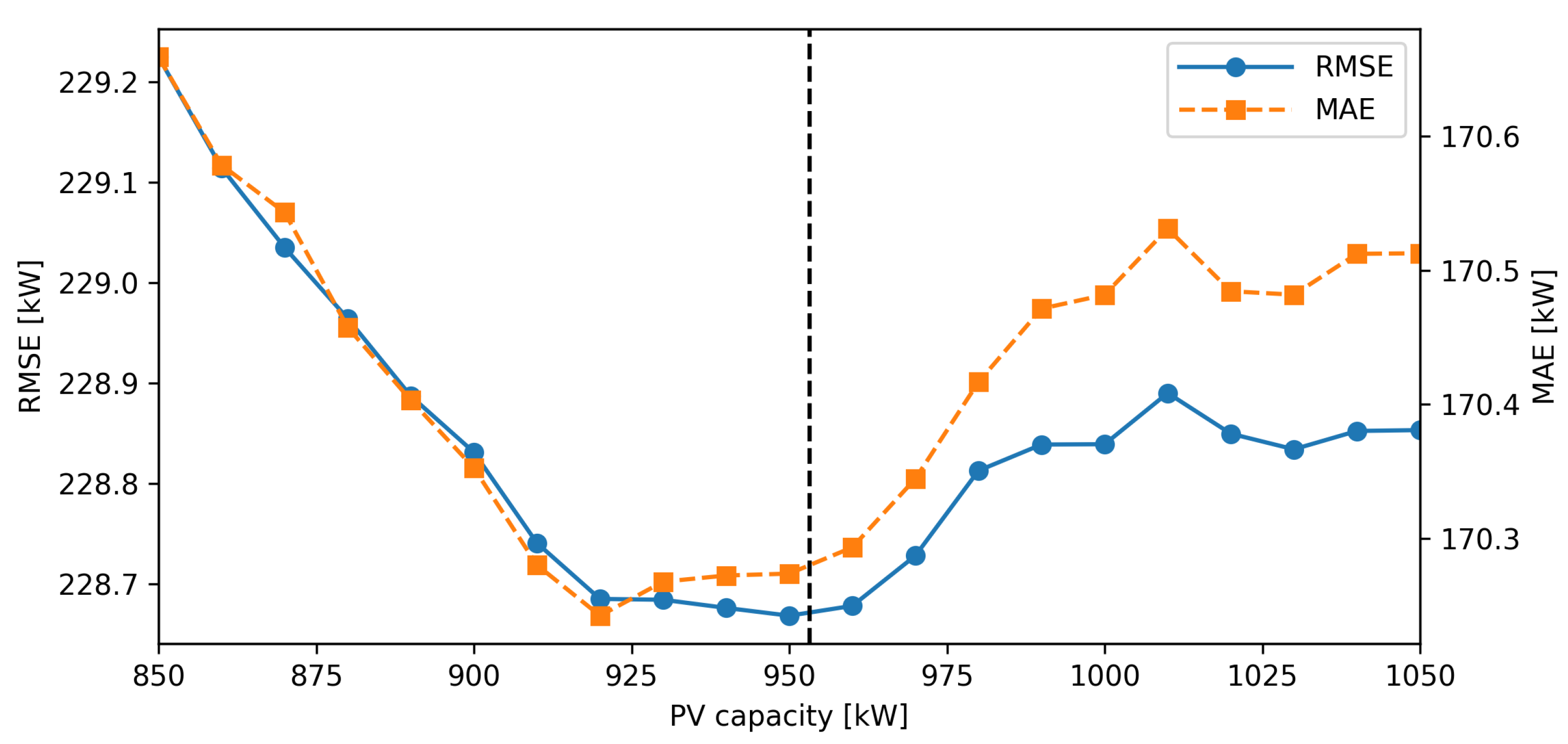
- how an estimate of the installed photovoltaic capacity can be inferred from the measured net power consumption and meteorological information;
- how—at least in this case—the use of separate models for the prediction of individual plants can yield better results than those obtainable by training a single regression model for the microgrid.
2. Data
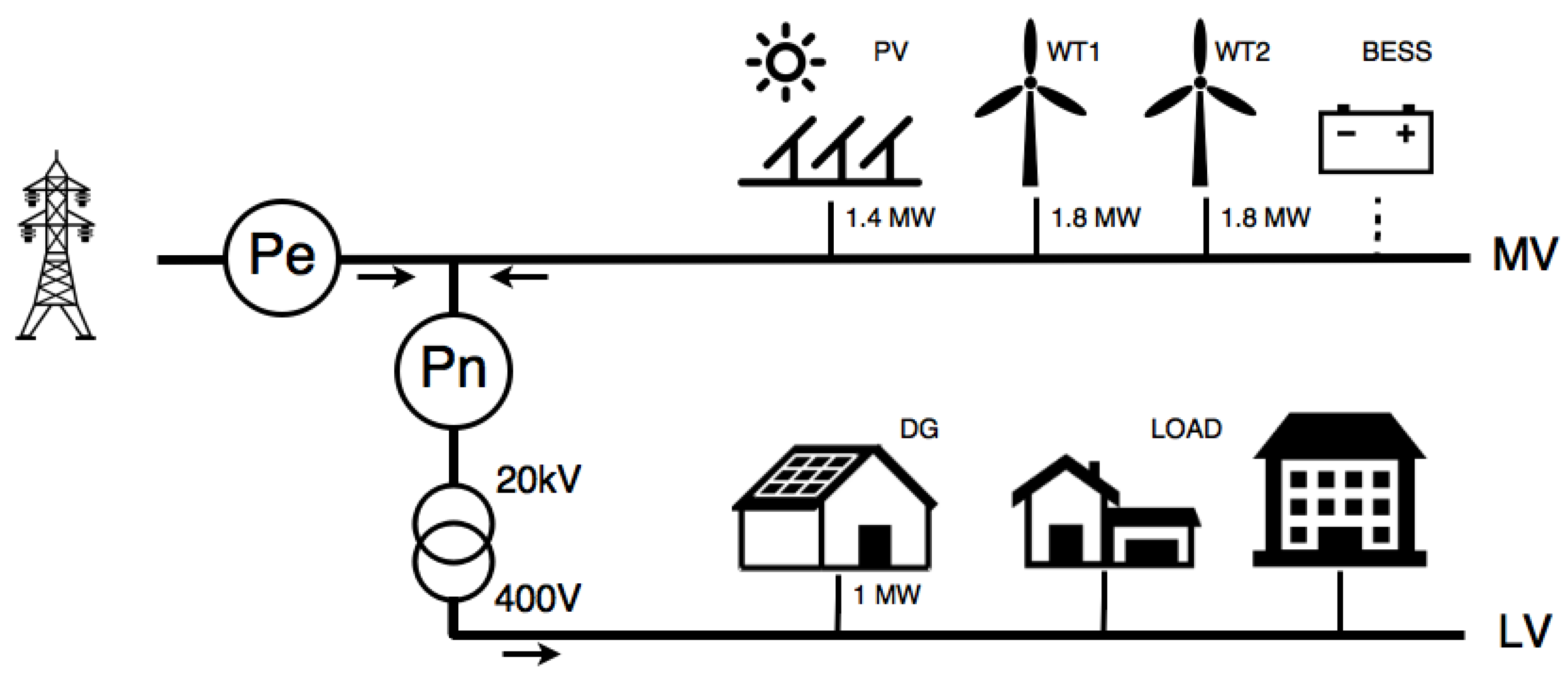
2.1. Borkum Grid
2.2. Weather Forecast
3. Method
3.1. Generated Power Forecast
3.2. Load Forecast
3.3. Power Exchange Forecast
4. Results and Discussion
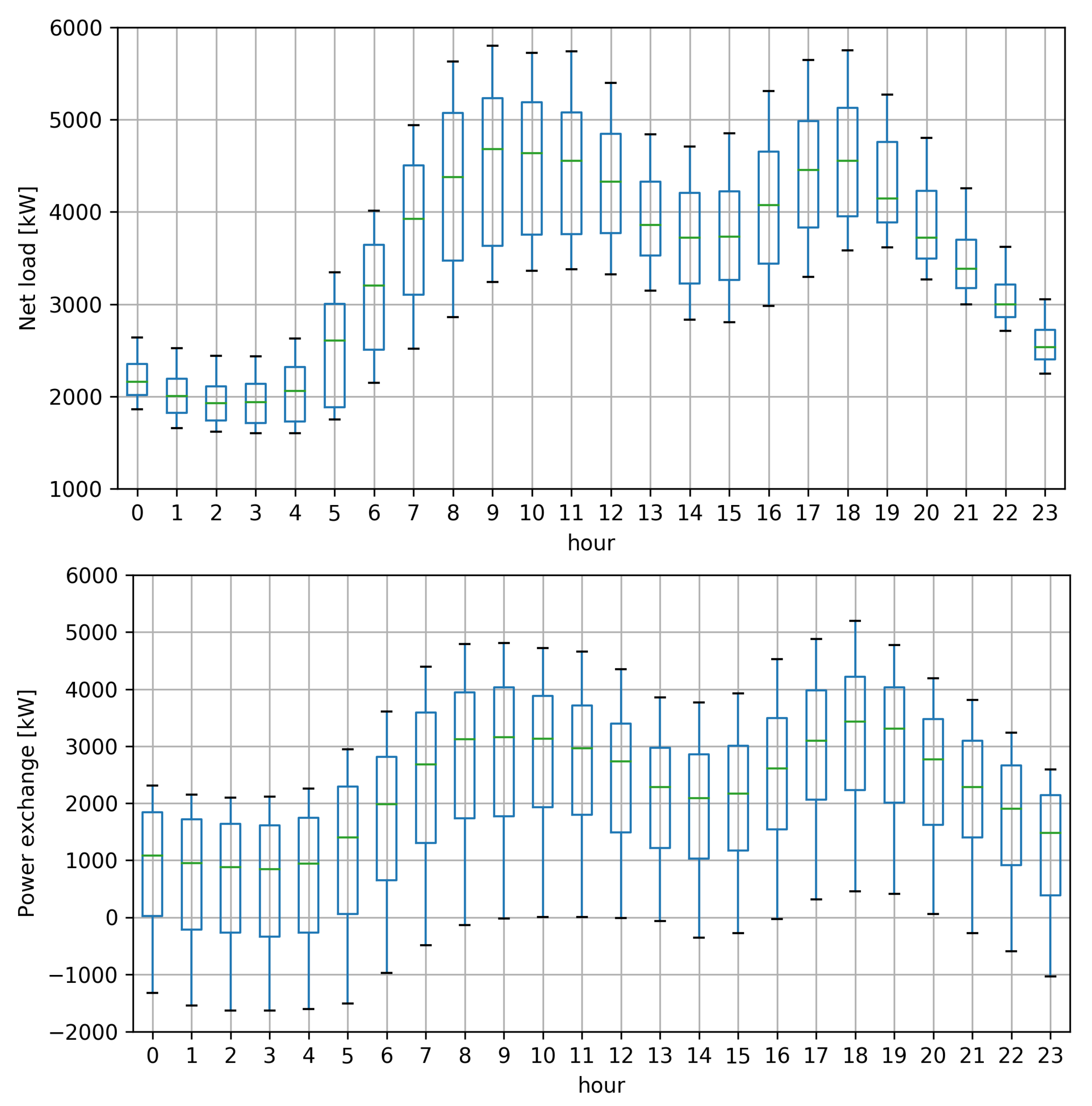
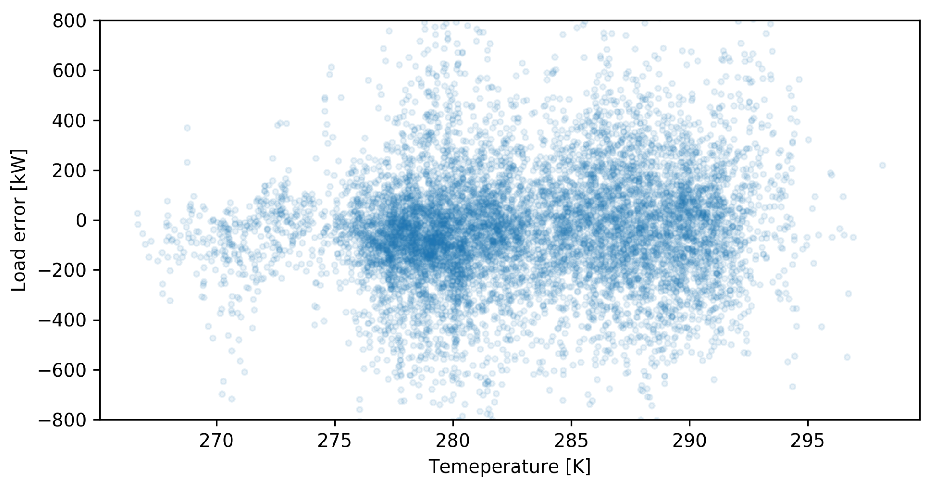
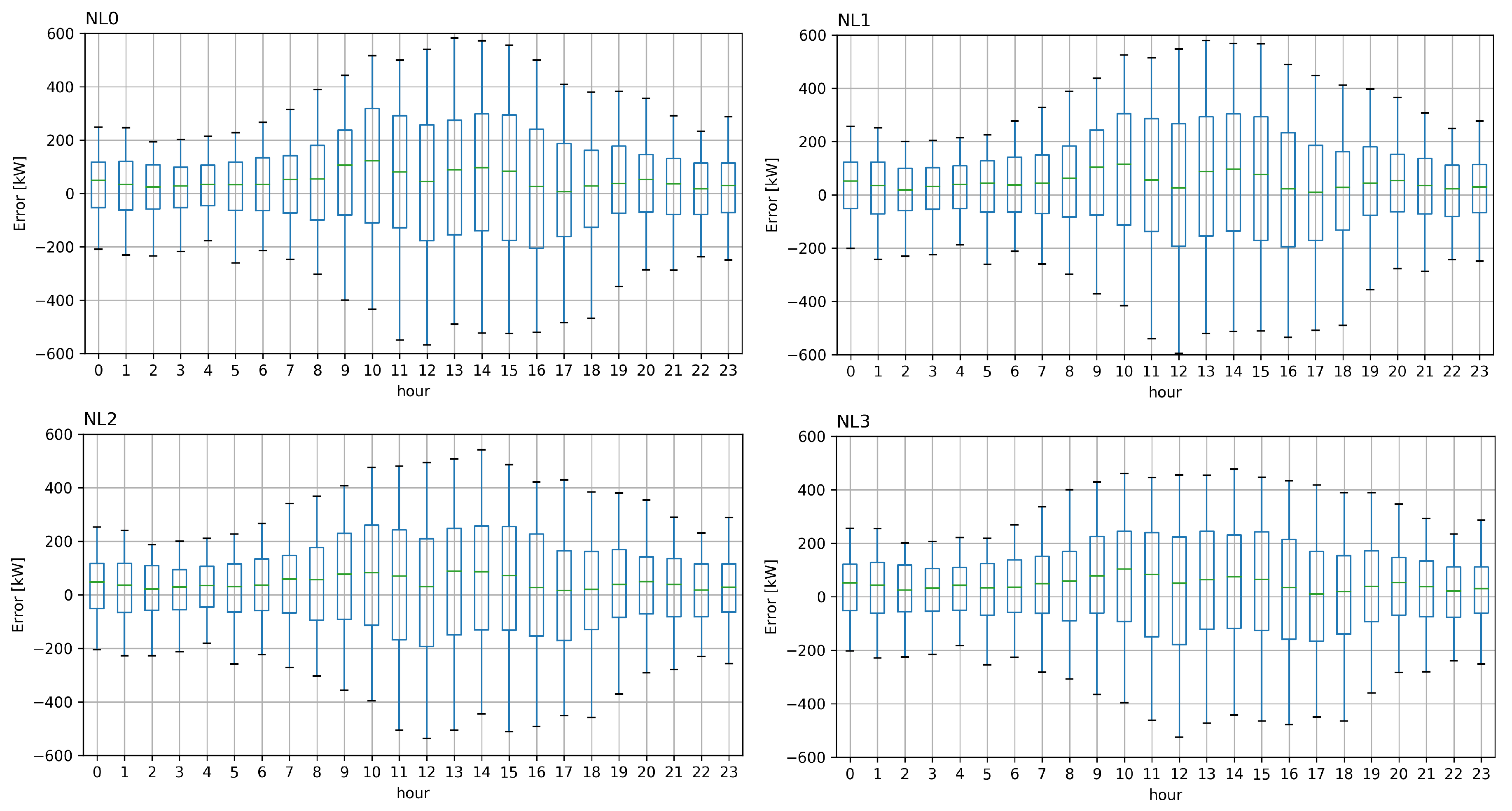
4.1. Load Forecast
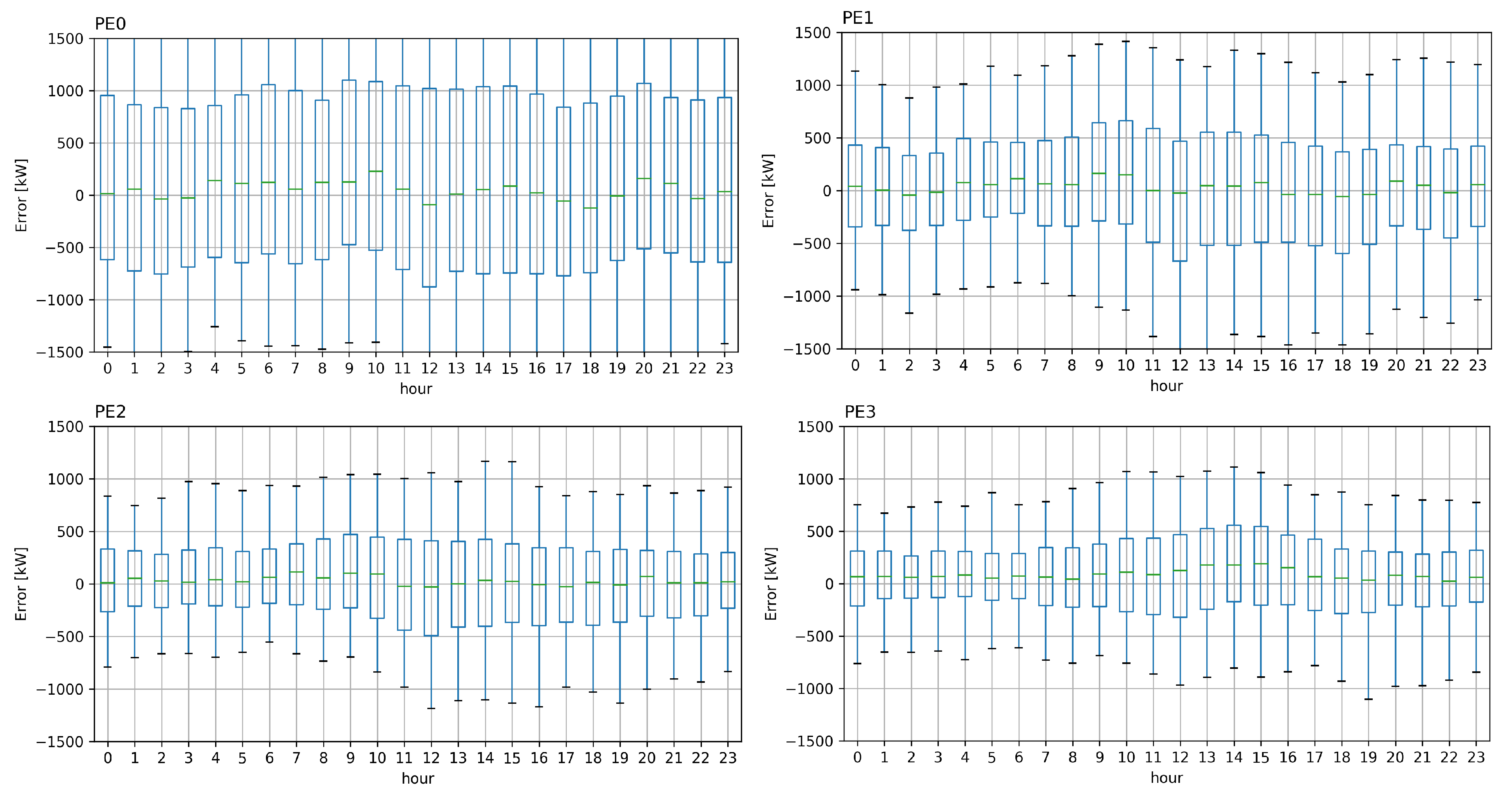
4.2. Power Exchange Forecast
5. Conclusions
Acknowledgments
Author Contributions
Conflicts of Interest
References
- Sepasi, S.; Reihani, E.; Howlader, A.M.; Roose, L.R.; Matsuura, M.M. Very short term load forecasting of a distribution system with high PV penetration. Renew. Energy 2017, 106, 142–148. [Google Scholar] [CrossRef]
- Zhao, H.; Wu, Q.; Hu, S.; Xu, H.; Rasmussen, C.N. Review of energy storage system for wind power integration support. Appl. Energy 2015, 137, 545–553. [Google Scholar] [CrossRef]
- Yuan, S.; Kocaman, A.S.; Modi, V. Benefits of forecasting and energy storage in isolated grids with large wind penetration—The case of Sao Vicente. Renew. Energy 2017, 105, 167–174. [Google Scholar] [CrossRef]
- Patra, S.; Kishor, N.; Mohanty, S.R.; Ray, P.K. Power quality assessment in 3-P grid connected PV system with single and dual stage circuits. Int. J. Electr. Power Energy Syst. 2016, 75, 275–288. [Google Scholar] [CrossRef]
- Kou, P.; Gao, F.; Guan, X. Stochastic predictive control of battery energy storage for wind farm dispatching: Using probabilistic wind power forecasts. Renew. Energy 2015, 80, 286–300. [Google Scholar] [CrossRef]
- Raza, M.Q.; Nadarajah, M.; Hung, D.Q.; Baharudin, Z. An intelligent hybrid short-term load forecasting model for smart power grids. Sustain. Cities Soc. 2017, 31, 264–275. [Google Scholar] [CrossRef]
- Sreekumar, S.; Verma, J.; Sujil, A.; Kumar, R. Comparative Analysis of Intelligently Tuned Support Vector Regression Models for Short Term Load Forecasting in Smart Grid Framework. Technol. Econ. Smart Grids Sustain. Energy 2017, 2, 1. [Google Scholar] [CrossRef]
- Feinberg, E.A.; Genethliou, D. Applied Mathematics for Restructured Electric Power Systems; Chapter-12, “Load Forecasting”; Springer: New York, NY, USA, 2005; pp. 269–285. [Google Scholar]
- Hahn, H.; Meyer-Nieberg, S.; Pickl, S. Electric load forecasting methods: Tools for decision making. Eur. J. Oper. Res. 2009, 199, 902–907. [Google Scholar] [CrossRef]
- Kyriakides, E.; Polycarpou, M. Short term electric load forecasting: A tutorial. Trends Neural Comput. 2007, 35, 391–418. [Google Scholar]
- Muñoz, A.; Sánchez-Úbeda, E.F.; Cruz, A.; Marín, J. Short-term forecasting in power systems: A guided tour. In Handbook of Power Systems II; Springer: New York, NY, USA, 2010; pp. 129–160. [Google Scholar]
- Singh, A.K.; Ibraheem; Khatoon, S.; Muazzam, M.; Chaturvedi, D.K. Load forecasting techniques and methodologies: A review. In Proceedings of the IEEE 2nd International Conference on Power, Control and Embedded Systems (ICPCES), Allahabad, India, 17–19 December 2012; pp. 1–10. [Google Scholar]
- Mirowski, P.; Chen, S.; Kam Ho, T.; Yu, C.N. Demand forecasting in smart grids. Bell Labs Tech. J. 2014, 18, 135–158. [Google Scholar] [CrossRef]
- Barak, S.; Sadegh, S.S. Forecasting energy consumption using ensemble ARIMA—ANFIS hybrid algorithm. Int. J. Electr. Power Energy Syst. 2016, 82, 92–104. [Google Scholar] [CrossRef]
- Hagan, M.T.; Behr, S.M. The time series approach to short term load forecasting. IEEE Trans. Power Syst. 1987, 2, 785–791. [Google Scholar] [CrossRef]
- Boroojeni, K.G.; Amini, M.H.; Bahrami, S.; Iyengar, S.; Sarwat, A.I.; Karabasoglu, O. A novel multi-time-scale modeling for electric power demand forecasting: From short-term to medium-term horizon. Electr. Power Syst. Res. 2017, 142, 58–73. [Google Scholar] [CrossRef]
- Singh, S.K.; Sinha, N.; Goswami, A.K.; Sinha, N. Several variants of Kalman Filter algorithm for power system harmonic estimation. Int. J. Electr. Power Energy Syst. 2016, 78, 793–800. [Google Scholar] [CrossRef]
- Taylor, J.W. Short-term electricity demand forecasting using double seasonal exponential smoothing. J. Oper. Res. Soc. 2003, 54, 799–805. [Google Scholar] [CrossRef]
- Bin, H.; Zu, Y.X.; Zhang, C. A Forecasting Method of Short-Term Electric Power Load Based on BP Neural Network. Appl. Mech. Mater. Trans. Tech. Publ. 2014, 538, 247–250. [Google Scholar] [CrossRef]
- Ghofrani, M.; Ghayekhloo, M.; Arabali, A.; Ghayekhloo, A. A hybrid short-term load forecasting with a new input selection framework. Energy 2015, 81, 777–786. [Google Scholar] [CrossRef]
- Men, Z.; Yee, E.; Lien, F.S.; Wen, D.; Chen, Y. Short-term wind speed and power forecasting using an ensemble of mixture density neural networks. Renew. Energy 2016, 87, 203–211. [Google Scholar] [CrossRef]
- Li, S.; Goel, L.; Wang, P. An ensemble approach for short-term load forecasting by extreme learning machine. Appl. Energy 2016, 170, 22–29. [Google Scholar] [CrossRef]
- Vaz, A.; Elsinga, B.; van Sark, W.; Brito, M. An artificial neural network to assess the impact of neighbouring photovoltaic systems in power forecasting in Utrecht, the Netherlands. Renew. Energy 2016, 85, 631–641. [Google Scholar] [CrossRef]
- Li, Y.; Wen, Z.; Cao, Y.; Tan, Y.; Sidorov, D.; Panasetsky, D. A combined forecasting approach with model self-adjustment for renewable generations and energy loads in smart community. Energy 2017, 129, 216–227. [Google Scholar] [CrossRef]
- Amarasinghe, K.; Marino, D.L.; Manic, M. Deep neural networks for energy load forecasting. In Proceedings of the IEEE 26th International Symposium on Industrial Electronics (ISIE), Edinburgh, UK, 19–21 June 2017; pp. 1483–1488. [Google Scholar]
- Vapnik, V.; Golowich, S.E.; Smola, A.J. Support vector method for function approximation, regression estimation and signal processing. In Proceedings of the 9th International Conference on Advances in Neural Information Processing Systems, Denver, CO, USA, 3–5 December 1996; pp. 281–287. [Google Scholar]
- Hong, W.C. Electric load forecasting by support vector model. Appl. Math. Model. 2009, 33, 2444–2454. [Google Scholar] [CrossRef]
- Humeau, S.; Wijaya, T.K.; Vasirani, M.; Aberer, K. Electricity load forecasting for residential customers: Exploiting aggregation and correlation between households. In Proceedings of the IEEE Sustainable Internet and ICT for Sustainability (SustainIT), Palermo, Italy, 30–31 October 2013; pp. 1–6. [Google Scholar]
- Chen, B.J.; Chang, M.W.; Lin, C.J. Load forecasting using support vector machines: A study on EUNITE competition 2001. IEEE Trans. Power Syst. 2004, 19, 1821–1830. [Google Scholar] [CrossRef]
- Niu, D.; Dai, S. A Short-Term Load Forecasting Model with a Modified Particle Swarm Optimization Algorithm and Least Squares Support Vector Machine Based on the Denoising Method of Empirical Mode Decomposition and Grey Relational Analysis. Energies 2017, 10, 408. [Google Scholar] [CrossRef]
- Marčiukaitis, M.; Žutautaitė, I.; Martišauskas, L.; Jokšas, B.; Gecevičius, G.; Sfetsos, A. Non-linear regression model for wind turbine power curve. Renew. Energy 2017, 113, 732–741. [Google Scholar] [CrossRef]
- Jung, J.; Broadwater, R.P. Current status and future advances for wind speed and power forecasting. Renew. Sustain. Energy Rev. 2014, 31, 762–777. [Google Scholar] [CrossRef]
- Antonanzas, J.; Osorio, N.; Escobar, R.; Urraca, R.; Martinez-de Pison, F.; Antonanzas-Torres, F. Review of photovoltaic power forecasting. Sol. Energy 2016, 136, 78–111. [Google Scholar] [CrossRef]
- Kaur, A.; Pedro, H.T.; Coimbra, C.F. Impact of onsite solar generation on system load demand forecast. Energy Convers. Manag. 2013, 75, 701–709. [Google Scholar] [CrossRef]
- Haupt, S.E.; Dettling, S.; Williams, J.K.; Pearson, J.; Jensen, T.; Brummet, T.; Kosovic, B.; Wiener, G.; McCandless, T.; Burghardt, C. Blending distributed photovoltaic and demand load forecasts. Sol. Energy 2017, 157, 542–551. [Google Scholar] [CrossRef]
- Reihani, E.; Sepasi, S.; Roose, L.R.; Matsuura, M. Energy management at the distribution grid using a Battery Energy Storage System (BESS). Int. J. Electr. Power Energy Syst. 2016, 77, 337–344. [Google Scholar] [CrossRef]
- Jin, L.; Cong, D.; Guangyi, L.; Jilai, Y. Short-term net feeder load forecasting of microgrid considering weather conditions. In Proceedings of the IEEE International Energy Conference (ENERGYCON), Dubrovnik, Croatia, 13–16 May 2014; pp. 1205–1209. [Google Scholar]
- Kaur, A.; Nonnenmacher, L.; Coimbra, C.F. Net load forecasting for high renewable energy penetration grids. Energy 2016, 114, 1073–1084. [Google Scholar] [CrossRef]
- Fonte, P.; Monteiro, C. Net load forecasting in presence of renewable power curtailment. In Proceedings of the IEEE 13th International Conference on the European Energy Market (EEM), Porto, Portugal, 6–9 June 2016; pp. 1–5. [Google Scholar]
- Shaker, H.; Zareipour, H.; Wood, D. Estimating power generation of invisible solar sites using publicly available data. IEEE Trans. Smart Grid 2016, 7, 2456–2465. [Google Scholar] [CrossRef]
- Zhang, X.; Grijalva, S. A Data-Driven Approach for Detection and Estimation of Residential PV Installations. IEEE Trans. Smart Grid 2016, 7, 2477–2485. [Google Scholar] [CrossRef]
- Wang, Y.; Zhang, N.; Chen, Q.; Kirschen, D.S.; Li, P.; Xia, Q. Data-Driven Probabilistic Net Load Forecasting with High Penetration of Invisible PV. IEEE Trans. Power Syst. 2017. [Google Scholar] [CrossRef]
- Persson, A. User Guide to ECMWF Forecast Products; Meteorological Bulletin 3; ECMWF: Reading, UK, 2001. [Google Scholar]
- Massidda, L.; Marrocu, M. Use of Multilinear Adaptive Regression Splines and numerical weather prediction to forecast the power output of a PV plant in Borkum, Germany. Sol. Energy 2017, 146, 141–149. [Google Scholar] [CrossRef]
- Marrocu, M.; Massidda, L. A simple and effective approach for the prediction of turbine power production from wind speed forecast. Energies 2017, 10, 1967. [Google Scholar] [CrossRef]
- Hor, C.L.; Watson, S.J.; Majithia, S. Analyzing the impact of weather variables on monthly electricity demand. IEEE Trans. Power Syst. 2005, 20, 2078–2085. [Google Scholar] [CrossRef]
- Drezga, I.; Rahman, S. Input variable selection for ANN-based short-term load forecasting. IEEE Trans. Power Syst. 1998, 13, 1238–1244. [Google Scholar] [CrossRef]
- Ruth, M.; Lin, A.C. Regional energy demand and adaptations to climate change: Methodology and application to the state of Maryland, USA. Energy Policy 2006, 34, 2820–2833. [Google Scholar] [CrossRef]


| Power Exchange | Net Load | |
|---|---|---|
| number | 105,216 | 105,216 |
| mean (kW) | 2029.5 | 3603.7 |
| std (kW) | 1600.7 | 1137.1 |
| min (kW) | 1446.2 | |
| max (kW) | 6651.2 | 6928.9 |
| Model | Variable | Technique | Features |
|---|---|---|---|
| PV | MARS | GHI, TCC | |
| WT | DM | WS100 | |
| MVF | Equation (2) | , | |
| NL0 | SVR | , , h, dow, doy, work, dst | |
| NL1 | SVR | , , , h, dow, doy, work, dst | |
| NL2 | SVR | , , , h, dow, doy, work, dst | |
| NL3 | SVR, Equations (3), (6) | , , , h, dow, doy, work, dst | |
| PE0 | SVR | , , h, dow, doy, work, dst | |
| PE1 | SVR | , , , , h, dow, doy, work, dst | |
| PE2 | SVR | , , , , , , h, dow, doy, work, dst | |
| PE3 | Equation (7) | , |
| Model | (-) | MAE (kW) | RMSE (kW) | nMAE (%) | nRMSE (%) | Q1 (kW) | Q3 (kW) |
|---|---|---|---|---|---|---|---|
| NL0 | 0.950 | 182.1 | 247.0 | 5.23 | 7.10 | 165.5 | |
| NL1 | 0.950 | 182.8 | 247.8 | 5.25 | 7.12 | 167.2 | |
| NL2 | 0.955 | 173.2 | 233.7 | 4.97 | 6.71 | 156.6 | |
| NL3 | 0.957 | 170.3 | 228.7 | 4.89 | 6.57 | 158.1 |
| Model | (-) | MAE (kW) | RMSE (kW) | nMAE (%) | nRMSE (%) | Q1 (kW) | Q3 (kW) |
|---|---|---|---|---|---|---|---|
| MVF | 0.820 | 336.5 | 482.4 | 22.16 | 31.76 | 188.7 | |
| PE0 | 0.375 | 971.4 | 1239.3 | 49.50 | 63.15 | 968.6 | |
| PE1 | 0.784 | 555.7 | 729.2 | 28.32 | 37.16 | 465.7 | |
| PE2 | 0.864 | 429.9 | 577.7 | 21.91 | 29.44 | 356.8 | |
| PE3 | 0.880 | 400.7 | 542.8 | 20.42 | 27.66 | 368.9 |
© 2017 by the authors. Licensee MDPI, Basel, Switzerland. This article is an open access article distributed under the terms and conditions of the Creative Commons Attribution (CC BY) license (http://creativecommons.org/licenses/by/4.0/).
Share and Cite
Massidda, L.; Marrocu, M. Decoupling Weather Influence from User Habits for an Optimal Electric Load Forecast System. Energies 2017, 10, 2171. https://doi.org/10.3390/en10122171
Massidda L, Marrocu M. Decoupling Weather Influence from User Habits for an Optimal Electric Load Forecast System. Energies. 2017; 10(12):2171. https://doi.org/10.3390/en10122171
Chicago/Turabian StyleMassidda, Luca, and Marino Marrocu. 2017. "Decoupling Weather Influence from User Habits for an Optimal Electric Load Forecast System" Energies 10, no. 12: 2171. https://doi.org/10.3390/en10122171
APA StyleMassidda, L., & Marrocu, M. (2017). Decoupling Weather Influence from User Habits for an Optimal Electric Load Forecast System. Energies, 10(12), 2171. https://doi.org/10.3390/en10122171