Article

Nuclear Power Learning and Deployment Rates; Disruption and Global Benefits Forgone

Centre for Applied Macroeconomic Analysis, Crawford School of Public Policy, Australian National University, Canberra, Australian Capital Territory 2601, Australia
Energies 2017, 10(12), 2169; https://doi.org/10.3390/en10122169
Submission received: 15 November 2017 / Revised: 10 December 2017 / Accepted: 12 December 2017 / Published: 18 December 2017
(This article belongs to the Section F: Electrical Engineering)

Abstract

:
This paper presents evidence of the disruption of a transition from fossil fuels to nuclear power, and finds the benefits forgone as a consequence are substantial. Learning rates are presented for nuclear power in seven countries, comprising 58% of all power reactors ever built globally. Learning rates and deployment rates changed in the late-1960s and 1970s from rapidly falling costs and accelerating deployment to rapidly rising costs and stalled deployment. Historical nuclear global capacity, electricity generation and overnight construction costs are compared with the counterfactual that pre-disruption learning and deployment rates had continued to 2015. Had the early rates continued, nuclear power could now be around 10% of its current cost. The additional nuclear power could have substituted for 69,000–186,000 TWh of coal and gas generation, thereby avoiding up to 9.5 million deaths and 174 Gt CO2 emissions. In 2015 alone, nuclear power could have replaced up to 100% of coal-generated and 76% of gas-generated electricity, thereby avoiding up to 540,000 deaths and 11 Gt CO2. Rapid progress was achieved in the past and could be again, with appropriate policies. Research is needed to identify impediments to progress, and policy is needed to remove them.

1. Introduction

Energy is the lifeblood of modern civilisation. Humans would still be hunter-gatherers if not for our ability to extract and use energy. Major advances in human wellbeing have been driven by transitions to cheaper and more plentiful energy. Examples include: the harnessing of fire, animals, wind and water power, and transitions from wood to coal, and from coal to oil and to gas [1,2,3,4]. A transition to cheaper, cleaner electricity globally would improve human wellbeing and reduce the environmental impacts of electricity generation [3,5,6,7,8].
People and businesses want cheap, reliable and secure energy. Globally, 1.2 billion people are still living without access to electricity [9]. According to the World Health Organisation (WHO) [8], “around 3 billion people cook and heat their homes using open fires and simple stoves burning biomass (wood, animal dung and crop waste) and coal”. WHO [7] estimated that 4.3 million deaths annually are attributable to indoor air pollution and 3.7 million to ambient (outdoor) air pollution. Gohlke et al. [6] found that increased electricity consumption per capita correlates with better health outcomes because of better access to clean water and sanitation, and reduced indoor and outdoor air pollution. They also found that access to a centralised power source is necessary to gain many of the benefits of clean power. Many of the deaths caused by indoor air pollution could be avoided if electricity replaced the burning of biomass and coal in homes, and many of the deaths attributable to outdoor air pollution could be avoided if clean technologies replaced fossil fuel for electricity generation.
Nuclear power produces comparatively little air or water pollution. Substituting nuclear for fossil fuel in electricity generation could prevent most of the deaths attributable to electricity generation. Cheap electricity increases productivity and economic growth, drives electrification for people without any electricity or with insufficient or unreliable electricity, and thereby more quickly raises living standards and human wellbeing. As the cost of electricity decreases, deployment rate increases. Transition takes place faster and the benefits are delivered sooner.
History is replete with examples of one technology replacing another [2,3]. Large infrastructure transitions have commonly taken around a century [10]. Examples are transitions to canals, railways, highways, oil and gas pipelines, telegraph, and electricity grids. Transitions typically follow an S-curve from 0 to 100% complete, with three phases: accelerating to about 20%, near-linear to about 80%, and decelerating to 100% [3,10]. Electricity grids reached 50% of world population in 1960 and 80% in 2010 [11].
The transition to nuclear power began in 1954 with the first reactor connected to the grid. Until the 1970s, it was envisaged that nuclear would emulate earlier energy transitions. For example, Wilson [12] projected that nuclear power would supply 14 to 21% of world primary energy by 2000. However, the transition to nuclear reached 4% by 1970, then stalled [3]. The deployment rate of nuclear capacity is currently less than in 1972; the transition has been stalled for 44 years.
The rate that technology transitions take place depends, in part, on the technologies being ‘fit-for-purpose’ and on the learning rates that occur during the transition period. To accelerate the transition to reliable, cheap, clean, safe and comparatively environmentally benign electricity generation, policies need to focus on ways to improve the learning rates and deployment rates of technologies that meet requirements. Historical learning rates provide insight into what rates may be achievable and what could be done to return to rapid rates.
The concept of learning rates, or cost experience curves [I], is widely used to quantify the rate at which costs reduce as experience is gained. Learning rate is the fractional reduction in cost per doubling of cumulative capacity or production. Rubin et al. [13] explain how to calculate learning rates, and summarise learning rates for selected electricity generation technologies. However, their paper has limited information on nuclear power learning rates, and none before 1972 or after 1996.
Lovering et al. [14] [II] provide a comprehensive analysis of nuclear power construction cost experience of early and recent reactors in seven countries; their analysis covers 58% of the reactors ever constructed for electricity generation, between 1954 and 2015. While there have been many studies of the cost escalation of nuclear power plants (e.g., [15,16], and others cited in Lovering et al. [14]), most are for the US and France only, and cover only periods since the 1970s. To the author’s knowledge, there are no comprehensive studies, other than Lovering et al. [14], that cover the full period of global commercial nuclear power reactor operation, nor any studies that provide the learning rates over the full period, and that highlight their reversal, which began in the late-1960s.
This study extends the literature by providing learning rates of nuclear power reactors for the seven countries analysed by Lovering et al. for the full period from 1954 through 2015. The aim is to answer two questions. What were the global benefits forgone as a consequence of the reversal of learning rates and the stalled deployment rates? What are the policy implications?
Using counterfactual analysis, Kharecha and Hansen [17] estimated that electricity generated by nuclear power avoided 1.84 million air-pollution-related deaths and 64 Gt of CO2 emissions between 1971 and 2009. The current analysis also uses a counterfactual approach. Lovering et al. data were re-analysed to calculate the historical learning rates and deployment rates of nuclear power, and to project the early rates to 2015. Evidence of disruption to the learning and deployment rates is presented and some of the benefits forgone are quantified. Estimates are presented for:
  • what the Overnight Construction Cost (OCC) [III],[IV] of nuclear power could have been in 2015 if the early learning and deployment rates had continued
  • the additional electricity that could have been generated by nuclear power if the early deployment rate trends had continued
  • the number of deaths and quantity of CO2 emissions that could thereby have been avoided.
The analysis finds that the benefits forgone because of the disruption, and the resulting stalled transition from fossil fuels to nuclear power, are substantial.
The purpose of this paper is to publish the evidence and the consequences of the disruption, and to suggest an approach to removing the impediments that are delaying progress. It does not explore the causes of the disruption and cost escalations thereafter; that would require extensive studies beyond the scope of this paper.
To summarise, this study provides learning rates for a full set of reactors in seven countries, covering builds from 1954 through to projects that had been completed by the end of 2015, covering 58% of all power reactors ever built globally. It also provides global deployment rates for that period. It estimates the extra electricity that could have been generated by nuclear power since 1980 and what OCC would have been in 2015 if the learning and deployment rates had not been disrupted. It compares the projections to the actuals to estimate forgone benefits of the disruption. It suggests an approach to removing the impediments that are retarding the transition to nuclear power.

2. Materials and Methods

This section explains the methods and assumptions used to:
  • calculate historical OCC learning rates
  • estimate the capacity of nuclear power that would have been constructed by 2015 if historical deployment rates had continued
  • estimate the OCC of nuclear power in 2015 by applying the pre-1970s learning rates to the capacities estimated from the projected deployment rates
  • estimate the quantity of extra electricity that could have been generated by nuclear power if the early deployment rates had continued to 2015; and the deaths and CO2 emissions that could thereby have been avoided.
Counterfactual analyses require simplifying yet tenable assumptions. As Kharecha and Hansen [17] explain for their counterfactual analysis of deaths and CO2 avoided by historical nuclear power deployment, “There are of course numerous complications involved in trying to design such a replacement scenario (e.g., evolving technological and socioeconomic conditions), and the … energy mix cannot be known with total accuracy and realism; thus, simplifying yet tenable assumptions are necessary and justified.” This study assumes, conservatively, that the historical electricity demand did not change (despite the reducing costs) and assumes that the additional electricity generated by nuclear power would have displaced equivalent coal and gas generation.
Costs are in 2010 US dollars as per Lovering et al. [14].

2.1. Learning Rates

The data of Lovering et al. [14] were re-analysed to calculate OCC learning rates. Figure 1 plots OCC ($/kW) against cumulative global capacity (GW) for the nuclear data points in Lovering’s Figure 13. There is a marked reversal in the slope of OCC against cumulative global capacity. Before cumulative global capacity reached around 32 GW, which occurred in 1967, OCC was decreasing as cumulative capacity increased (i.e., learning rates were positive). Then an abrupt change occurred; thereafter, OCC was increasing (i.e., learning rates were negative). The trendlines are fitted to the US data points before and after 32 GW to highlight the dramatic reversal.
Given this evidence for two phases, learning rates were calculated for two periods, that is, before and after the slope reversal, for each country. The reversal occurred at different times in different countries and regions. It occurred first in the US; there was a lag to Canada and Europe and a further lag to Asia. The reversal points selected were: 32 GW for US; 64 GW for Canada, France and Germany; 100 GW for Japan; and 128 GW for India; there is no reversal point for South Korea because it had no construction starts before 1972, so no pre-reversal data points.
The data points were plotted on log-log axes (base 2), trendlines fitted to the pre- and post-reversal periods for each country, and learning rates calculated for each trendline. Following Rubin et al. [13], learning rates were calculated by regressing OCC against cumulative global capacity using a power function. Learning rate is equal to 1–2b where b is the exponent of the fitted power function.

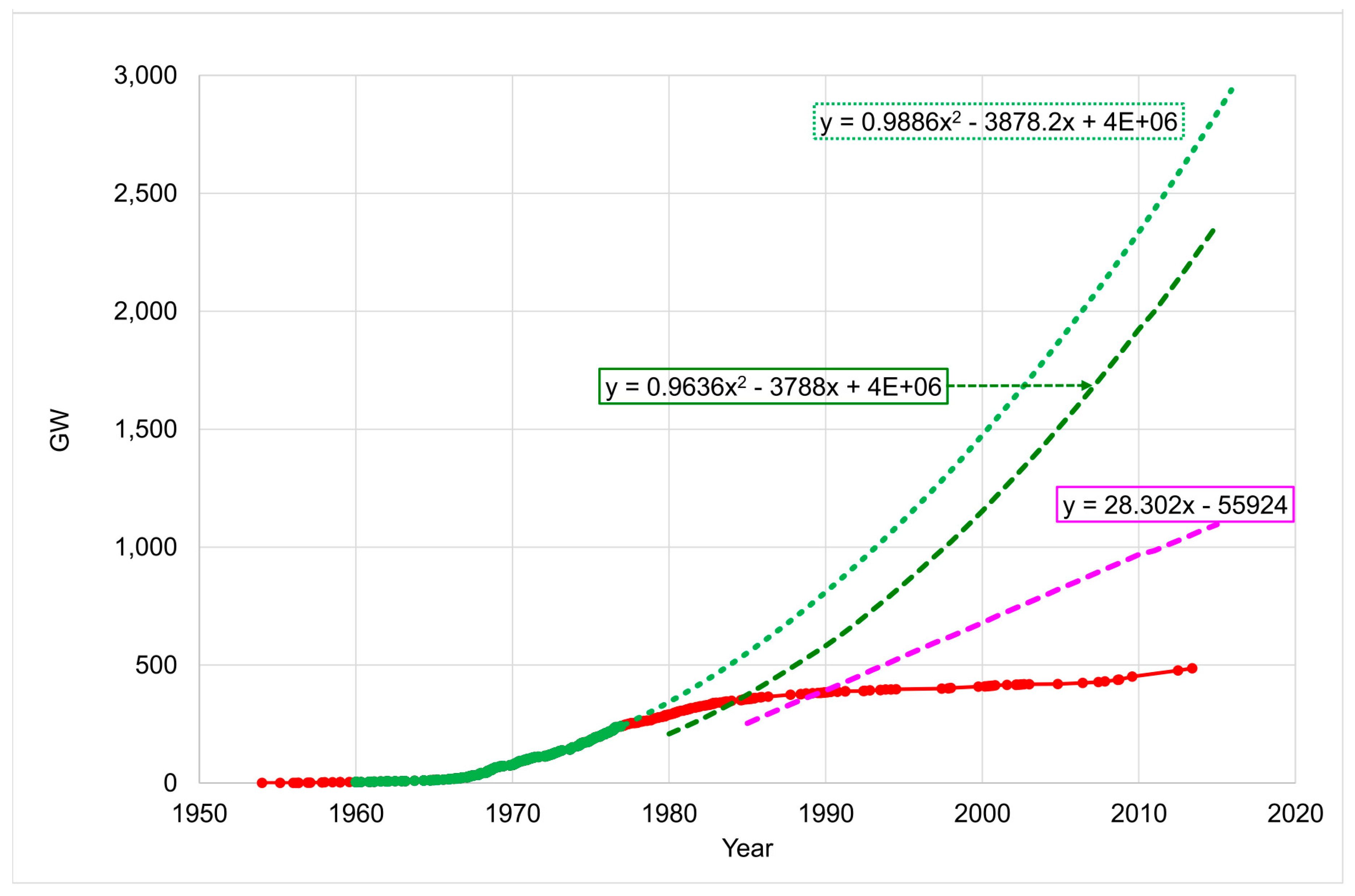
2.2. Deployment Rate Projections

To calculate the OCC of nuclear power in 2015 requires a projection of what the cumulative global capacity of construction starts would have been. Similarly, to calculate the extra electricity that would have been generated at the higher deployment rates, and the deaths and emissions that could have been avoided, requires a projection of what the global capacity of operating reactors would have been. This projection assumes that, if not for the disruption, the construction period would have been five years [V] and the capacity of power uprates and of reactors permanently shut down each year would have been unchanged from the actual. Three deployment rate scenarios were analysed: the actual historical rate and two projections of early historical rates:
Actual: This is the actual historical deployment from 1954 to 2015. The cumulative global capacity of construction starts was 486 GW in 2013 [14]; 11 GW was added in 2014 and 2015, making the total 497 GW in 2015. The actual global capacity in operation in 2015 was 383 GW [18] [VI].
Linear: The capacity of commercial operation starts peaked at 40 GW in 1985 and averaged 30 GW per year from 1984 to 1986 [18]. The capacity in commercial operation in 1985 was 253 GW [19]. The Linear scenario assumes that commercial operation starts continued at 30 GW per year from 1985 to 2015, and the capacity of power uprates and reactors permanently shutdown each year was as per the historical data. (See Appendix A for further explanation of the calculation method and data sources.)
Accelerating: From 1954 to 1976, the capacity of construction starts was accelerating, then slowed in 1976 (i.e., about 5 to 10 years after the reversal points, which was when OCC started to increase rapidly). If the OCC had continued to reduce at the pre-reversal learning rates, it was assumed the deployment rate also would have continued (all else being equal). A defensible assumption is that the rate continued at that prevailing from 1960 to 1976. A polynomial function was fitted to the data points for 1960 to 1976 and projected to 2015. The cumulative global capacity of commercial operation starts was estimated by subtracting five years (for the assumed average construction duration) from the cumulative global capacity of construction starts and subtracting the actual capacity of reactors permanently shut down (see Appendix A for further explanation).
The Linear and Accelerating scenarios are used to estimate the extra electricity that would have been supplied each year by nuclear power from 1985 to 2015 (for the Linear) and from 1980 to 2015 (for the Accelerating) scenarios.

2.3. Projected Overnight Construction Costs in 2015

OCC in 2015 was calculated for the three deployment rate scenarios by applying the pre-reversal learning rates to the 2015 actual capacity and to the two projections, i.e., by substituting the actual and projected capacity in 2015 in the trendline equations (shown in Figure 2 for each country).
The projected OCC in 2015 were compared with the actuals. IEA [20] published estimates (in 2013 USD) of actual OCC for nuclear power (as well as other technologies) for US, France, Japan and Korea. Here, these were adjusted to 2010 USD for consistency with Lovering et al. using the World Bank GDP deflator [21]. IEA [20] includes OCC for twenty two countries, but not for Canada, Germany and India, so $4000 was assumed for Canada, $5000 for Germany, and $2000 for India. These figures are close to OCC for US, France and Korea respectively, and are approximately consistent with the OCC of the last construction starts for those countries (Figure 2).

2.4. Extra Nuclear Electricity, Avoided Deaths and CO2

The number of deaths and the quantity of CO2 emissions that could have been avoided with the Linear and Accelerating scenarios were estimated. The extra nuclear electricity generated was estimated by factoring up the historical global annual nuclear net generation [22] in proportion to projected capacity divided by actual capacity [19]. (See Appendix A.)
To calculate the deaths and CO2 emissions that could have been avoided, it was assumed the extra electricity generated by nuclear substituted for coal generation in the Linear scenario and for coal and gas generation in the Accelerating scenario, with conversion factors [VII]:
  • Deaths: Coal = 60/TWh [VIII], Gas = 4/TWh (Wang [23]).
  • CO2 emissions: Coal = 1 Mt/TWh, Gas = 0.6 Mt/TWh (Kharecha and Hansen [17])
This study conservatively adopts the historical demand profile (despite the declining cost). Appendix A explains the calculations and data sources.

3. Results and Discussion
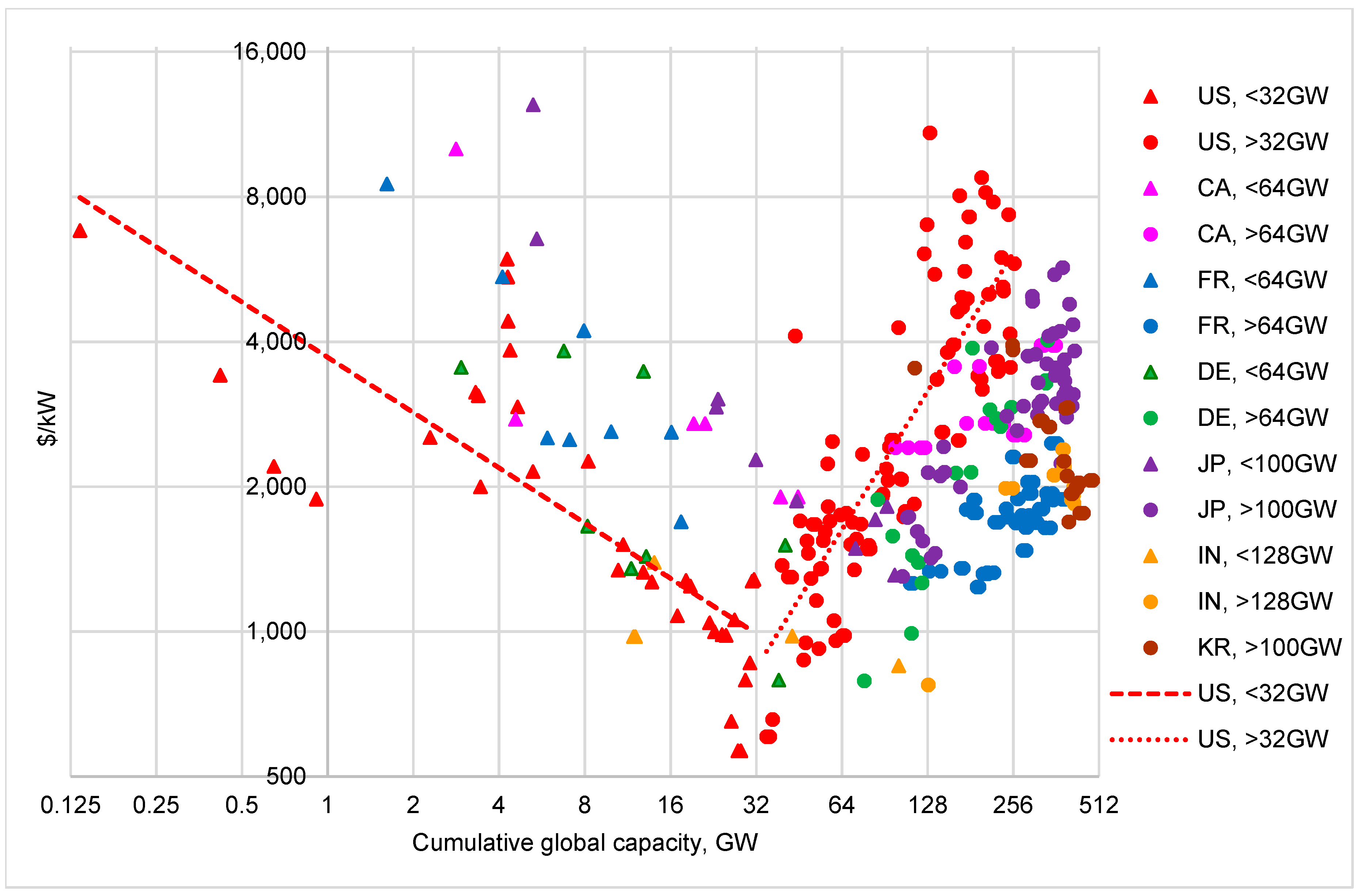
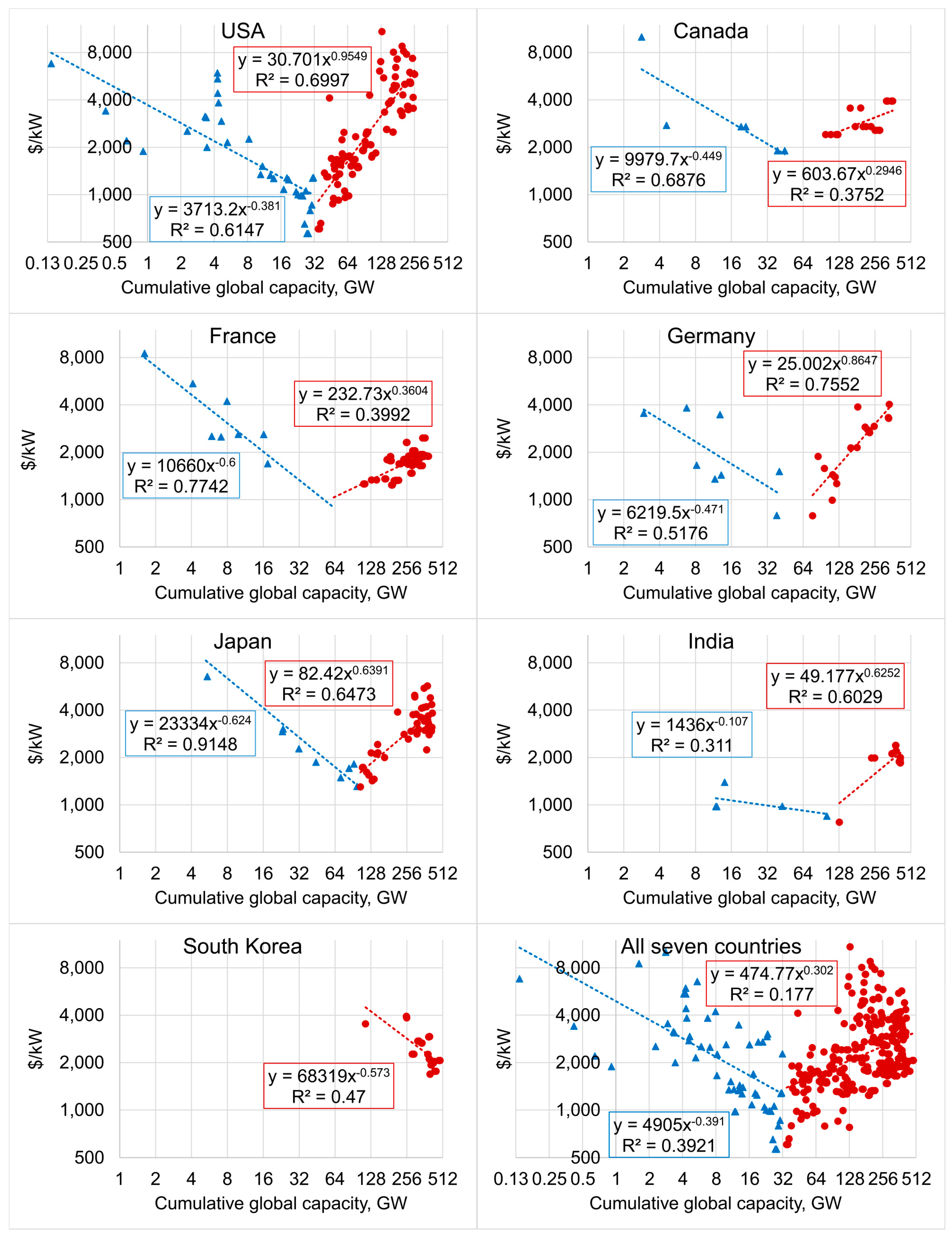
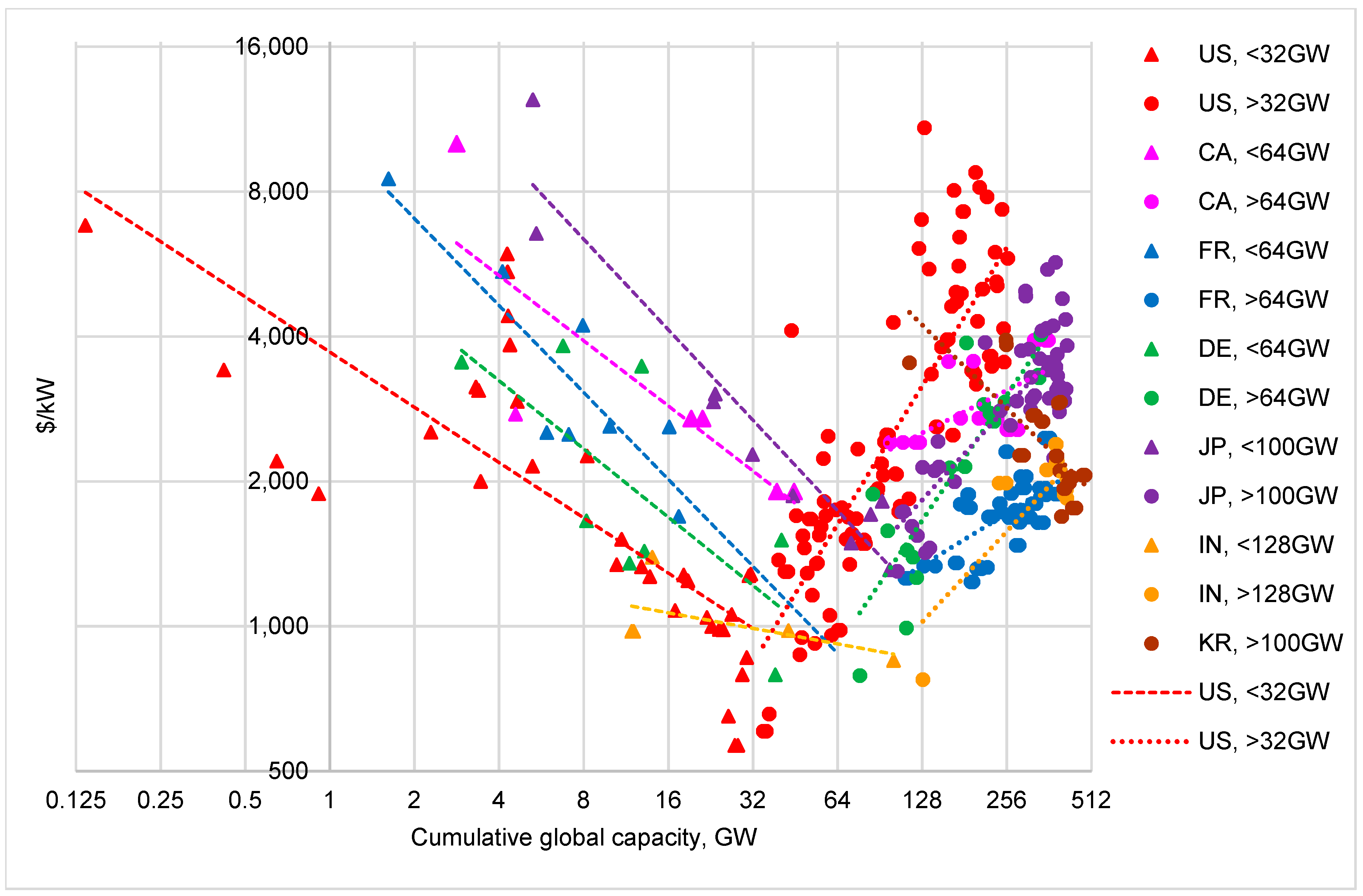
3.1. Learning Rates

Figure 2 has a chart for each of the seven countries and one for all seven combined; trendlines were fitted to the data points before and after the trend reversal points. The equation for each trendline is shown on the charts.
Figure 2. OCC (2010 US $/kW) plotted against cumulative global capacity (GW) of nuclear power reactors, based on construction start dates; regression lines fitted to points before and after trend reversals.
Energies 10 02169 g002
To compare trends for the seven countries, Figure 3 shows all the regression lines. Japan and France had the fastest pre-reversal learning rate; South Korea had a similar rate since it started building reactors in 1972, although it started from a high OCC after the reversal and initial rapid cost escalation in the other countries.
Table 1 lists the learning rates for both periods in each country for both the cumulative global and the cumulative country capacity. The sixth and seventh columns are the selected reversal point (cumulative global capacity of construction starts, and approximate year it occurred) for each country. The last column is the projected OCC at 497 GW cumulative global capacity if the pre-reversal learning rates had continued.
Learning rates are affected by the growth of cumulative capacity both globally and locally. Following Lovering et al., cumulative global capacity was used as the reference. Figure 4 plots the learning rates against the time span of the construction starts for each period in each country.
Table 1 and Figure 4 show that, before the reversal, OCC learning rates were 23% in the US, 27% to 35% in the other countries except India (where it was 7%), and 24% for all countries combined. At the reversal, learning rates changed abruptly and became negative (−94% in the US, −82% in Germany, −23 to −56% in the other countries, except in South Korea, and −23% for all seven countries); South Korea started building nuclear power plants after the initial rapid cost-escalation period, achieving a 33% learning rate since 1972. The fact that fast learning rates existed up to about 1970, and in South Korea since, suggests they could be achieved again [IX].
The US’s post-reversal learning rate was the worst of the seven countries. The reversal occurred one to five years later in the other countries and the real cost increase was not as severe as in the US. This suggests the US may have negatively influenced the development of nuclear power in all seven countries (and probably all countries). It also shows that technology learning and transition rates can change quickly and disrupt progress, in this case delaying progress for about half a century so far.

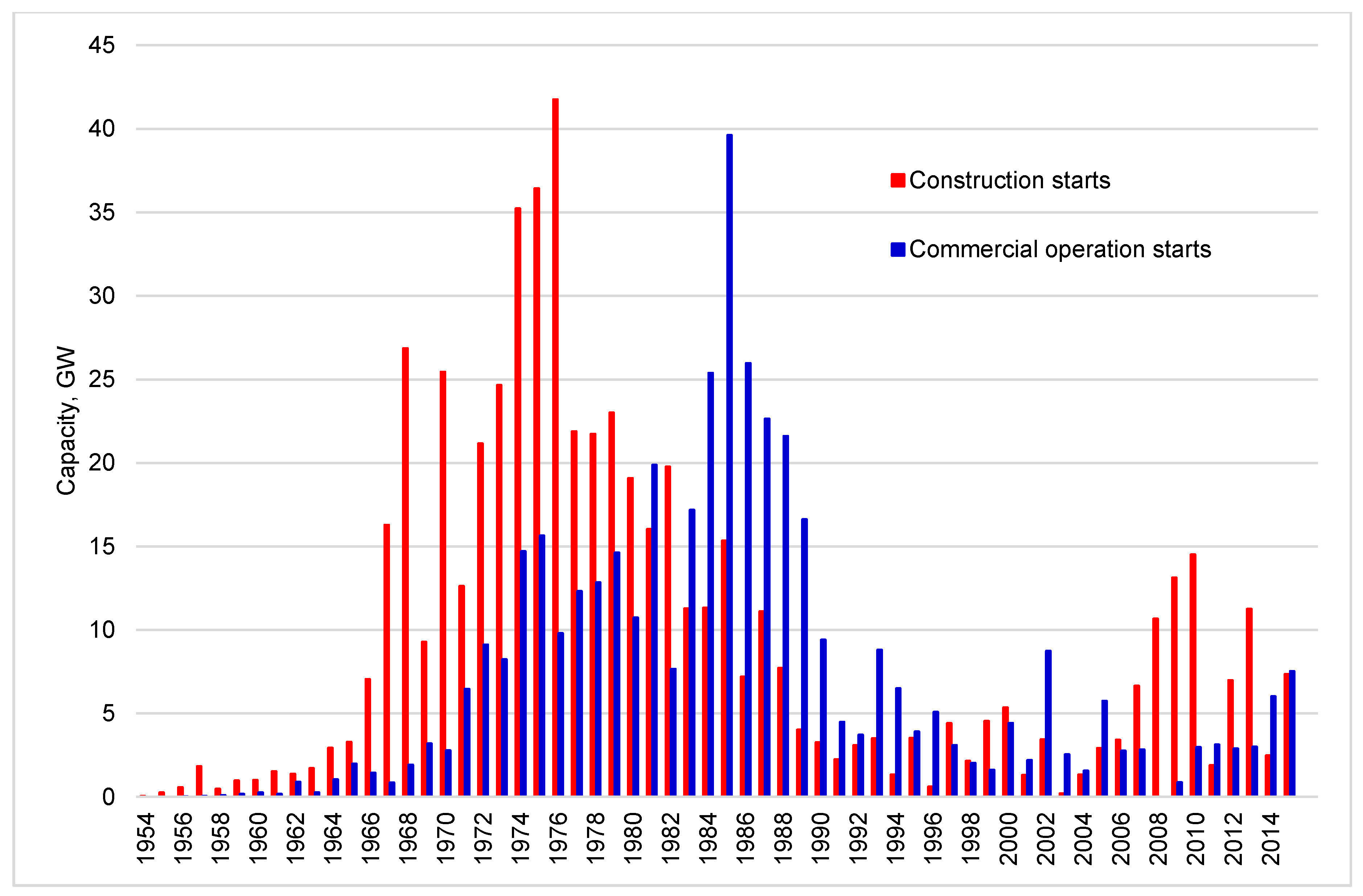
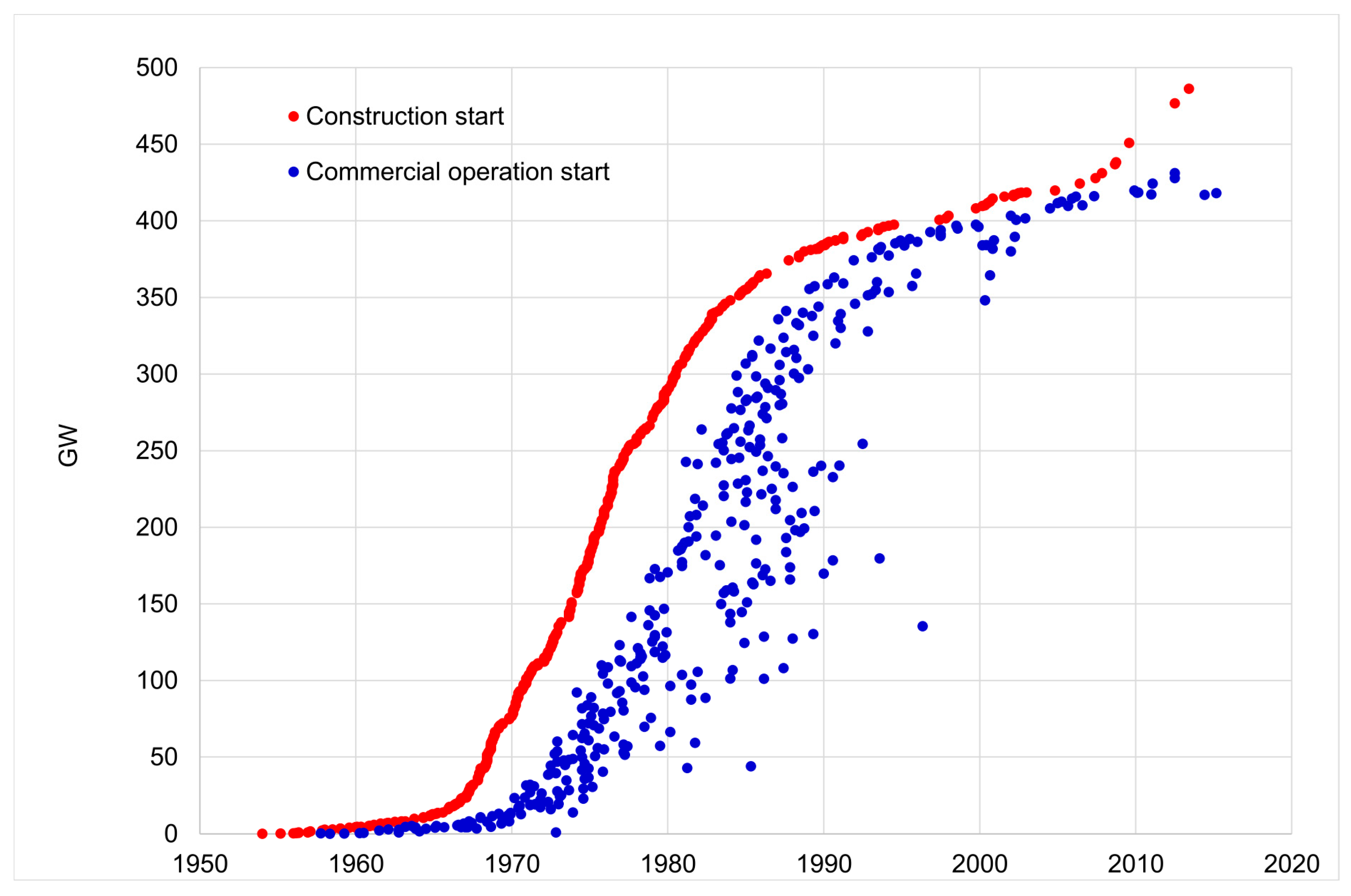
3.2. Deployment Rates and Projections to 2015

Figure 5 shows the annual global capacity of construction starts [X] and commercial operation starts from 1954 to 2015 [18]. The capacity of construction starts was accelerating until about 1970, peaked in 1976, then stalled. The annual capacity of commercial operation starts peaked in 1985, averaged 30 GW per year from 1984 to 1986, then declined rapidly and has not recovered. IAEA [24] shows grid connections peaked at 31 GW per year in 1984 and 1985 and declined rapidly thereafter.
Figure 6 shows cumulative global capacity of construction starts and commercial operations starts plotted against time (top panel), and projections of what they would have been in 2015 if the early deployment rates had continued (bottom panel).
Table 2 summarises the cumulative global capacity of actual and projected construction starts and the capacity in commercial operation at the end of 2015 for each scenario.
The Linear and Accelerating projections of cumulative global capacity by 2015 in Table 2 represent scenarios calculated on the basis of the stated deployment rate assumptions. The increases in projected cumulative global capacity by 2015 compared with Actual are large. It is useful to compare these scenarios with projections made in the 1970s. For example, the Accelerating deployment rate projects a global nuclear capacity of 1152 GW by 2000. The Workshop on Alternative Energy Strategies (WAES) [12], projected global nuclear capacity in 2000 at between 913 GW and 1722 GW [XI]. So the present projection is quite consistent with the outlook of 40 years ago.

3.3. Projected Overnight Construction Costs in 2015

Table 3 lists the projected OCC in 2015 and the percentage reduction from the actual OCC [20] for the six countries that were constructing reactors before the learning rate reversals. Actual OCC for Canada, Germany and India are approximate, as noted in Section 2.3.
If the pre-reversal learning rates had continued, with the Actual deployment unchanged, until 2015 when cumulative global capacity of construction starts was 497 GW, the OCC of nuclear power would be 5 to 15% of what it was in 2015 (except in India); for example, the OCC would be $349/kW in the US, $257/kW in France, and $484/kW in Japan (Table 3). These are much lower than the OCC of fossil fuel and other alternative electricity generation technologies [20].
If the pre-reversal learning rates and the Linear and Accelerating deployment rates had continued, the OCC would be approximately 2% to 10% of what it was in 2015 (except in India where it would be 31 to 33%) (Table 3).
These are striking cost reductions that, to be achieved, would have required pre-reversal learning rates and deployment rates to continue. If the rapid learning and deployment rates that prevailed pre-reversal could be achieved again, nuclear power would become much cheaper than fossil fuel technologies in the future. Some may regard this as too optimistic. However, there is no apparent physical or technical reason why they could not have continued and cannot prevail again. They have prevailed in South Korea over the past 40 years (Figure 4), and there are examples in other complex technologies and industries of cost reductions at similar rates that persisted over the past 50 years at the same time as the OCC of nuclear power was increasing rapidly [XII].

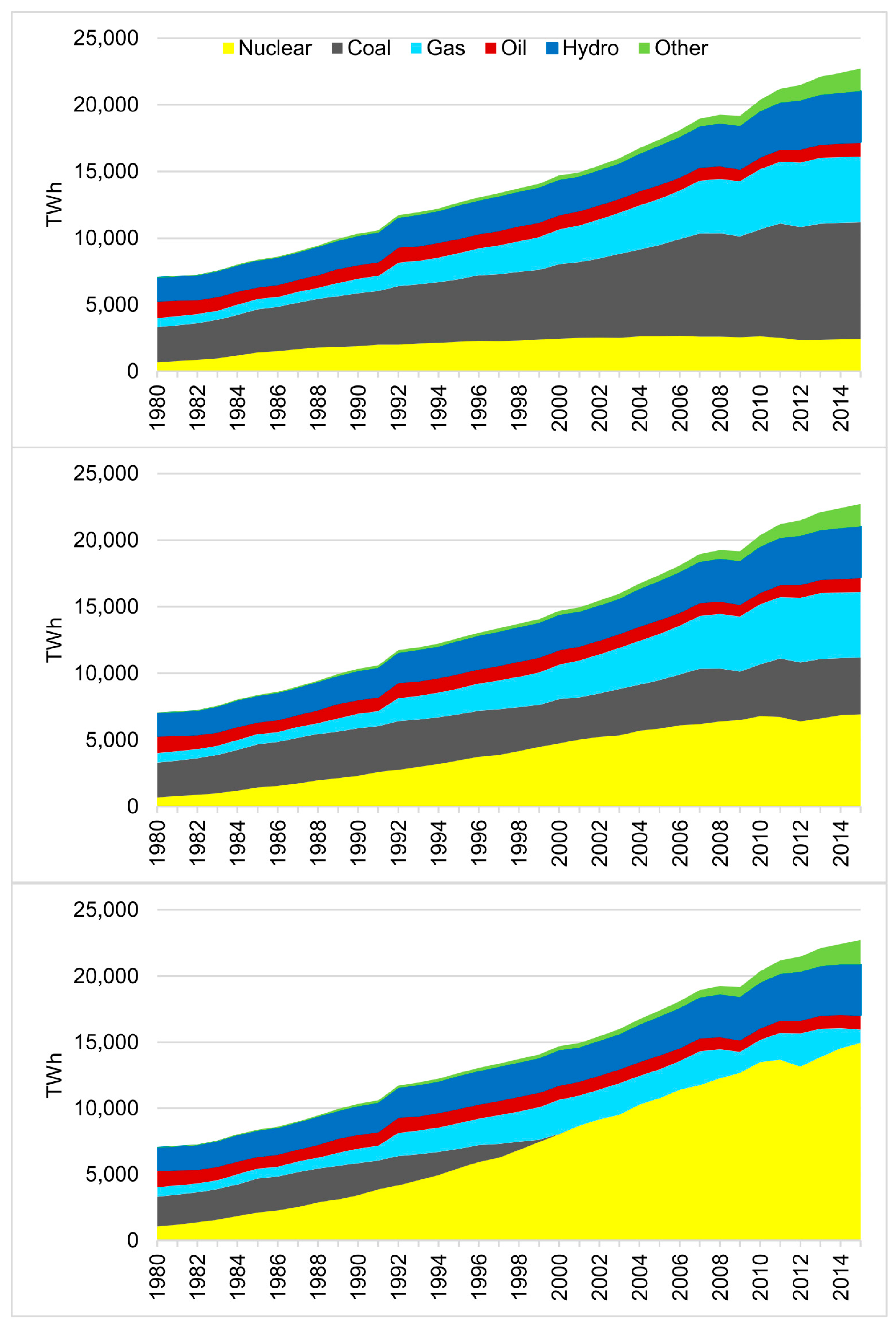
3.4. Extra Nuclear Electricity, Avoided Deaths and CO2

Figure 7 shows the annual electricity generated by fuel type for the three deployment rate scenarios: Actual, Linear and Accelerating.
Table 4 shows that, at the Linear deployment rate, the extra nuclear generation from 1985 to 2015 could have substituted for 69,000 TWh of mostly coal-generated electricity globally and avoided approximately 4.5 million deaths (from outdoor air pollution and all other causes in the respective energy chains, but not including deaths that could have been avoided by increasing access to clean water and sanitation services) and 69 Gt CO2 emissions.
At the Accelerating rate, the extra nuclear generation could have exceeded the actual generation from coal by year 2000 (assuming electricity demand did not change). If the extra nuclear generated electricity had substituted for coal and gas generation, about 9.5 million deaths and 174 Gt CO2 may have been avoided.
In 2015 alone, if the extra nuclear generation had replaced coal and gas generation, and electricity demand was unchanged, nuclear could have:
  • substituted for 49% of coal-generated electricity, thus avoiding 273,000 deaths and 4.5 Gt CO2 emissions (Linear scenario)
  • substituted for 100% of coal- and 76% of gas-generated electricity, thus avoiding 540,000 deaths and 11 Gt CO2 emissions (Accelerating scenario) [XIV].

3.5. Other Benefits Forgone

If the pre-reversal learning rates had continued, OCC, and consequently the cost of electricity, would undoubtedly have declined. Arguably this would have led to other benefits not estimated in this analysis, such as increased productivity, faster economic growth, improved standard of living, and better health and education outcomes.
The declining cost of electricity would probably have caused increasing demand and consumption. Substitution of electricity for fossil fuels for heat and transport may have proceeded faster. With declining costs and increasing demand, electricity grids may have expanded faster with more people being connected. Alstone et al. [11] charts the world population and the number of people who were connected to an electricity grid for the period 1830 to 2013. If grid connections had continued to accelerate at the rate that prevailed between 1950 and 1975, many of the 1.2 billion people who were not grid-connected in 2015 could have been.
With increased consumption, electricity could have substituted for some combustion of fuels by the 3 billion people who cook and heat their homes using open fires and simple stoves burning wood, animal dung, crop waste and coal, thereby reducing the 4.3 million deaths per year attributable to indoor air pollution [7]. And clean water and sanitation systems could have been provided to more people, reducing deaths from contaminated water [6].
The benefits forgone may have been substantially greater than estimated in the present counterfactual analyses. World energy consumption slowed in the 1970s [3] and GDP growth rate slowed too [25]. If the transition from fossil fuels to nuclear power had not been disrupted, world GDP growth may not have slowed as much. The global economy could have been significantly different from what it is now.

3.6. Policy Implications

Policies that increase the real cost of energy would be damaging economically, and are unlikely to be politically sustainable and, therefore, unlikely to succeed in the long term. To reduce the emissions that are detrimental to health and the environment, countries will need access to low-emissions technologies that are cheaper than high-emissions technologies. In this case, carbon pricing and command-and-control policies, such as incentives for low emissions and penalties for high emissions technologies, would not be required.
Cheap electricity increases productivity and economic growth, drives faster electrification for the people without access to electricity or with insufficient and/or unreliable electricity, and thus more quickly lifts the world’s population to higher living standards. As electricity costs decrease, the deployment rate increases and capacity doublings occur faster. Consequently, costs reduce faster; i.e., we progress more quickly down the learning curve [XV] [26]. Technology transition takes place faster and the benefits are delivered sooner.
These benefits could be achieved in the future if the impediments that disrupted the transition to nuclear power are removed. While this paper does not attempt to discuss the causes of the disruption and cost escalations thereafter, many others have (e.g., Cohen [15], Grubler [16], and Lovering et al. [14] cites a number of studies). A likely root-cause of many of the causes discussed in the literature was the growing concern about the safety of nuclear power, fanned by the anti-nuclear protest movement, which began in the mid-1960s (Daubert and Moran [27]; Wyatt [28]), and the ongoing political, legislative and regulatory responses to the concerns.
The fact that rapid learning and deployment rates prevailed in the past suggests they could be achieved again. To achieve them, it is suggested four steps are needed:
  • First, recognise that the disruption to the transition occurred and the impediments to progress continue to this day.
  • Second, recognise the consequences of the disruption for the global economy, human wellbeing and the environment, and the ongoing delays to progress.
  • Third, identify the root causes of the disruption and cost escalations since, and the solution options.
  • Fourth, implement policies to remove impediments that are retarding the transition.
The benefits forgone cannot be recovered, but future benefits can be increased by amending the policies that caused the cost increases and slowed the deployment of nuclear power. Human wellbeing could improve faster if the impediments that are slowing the development and deployment of nuclear power are removed.

4. Conclusions

From 1954 to the late-1960s, learning rates of nuclear power OCC were positive (i.e., OCC decreased as capacity increased). In the late-1960s, learning rates turned negative (i.e., OCC increased as capacity increased) and have remained negative ever since in all the seven countries analysed, except South Korea.
The disruption to learning rates was followed by stalled deployment rates.
If the pre-1970s learning rates had continued, and assuming the actual deployment did not change, OCC of nuclear power in 2015 could have been around 5 to 15% of what it actually was.
If both the pre-1970s learning rates and the Linear or Accelerating deployment rates had continued, OCC in 2015 could have been around 2 to 10% of actual.
If deployment had continued to add 30 GW to global capacity per year since 1985, 69,000 TWh of extra nuclear electricity could have been generated. Assuming this replaced coal-fired electricity generation, 4.2 million deaths and 69 Gt CO2 may have been avoided.
If deployment had continued from 1976 at the Accelerating rate that prevailed from 1960 to 1976, 186,000 TWh of extra nuclear electricity could have been generated. Assuming this extra nuclear generation replaced coal- and gas-powered electricity generation, 9.5 million deaths and 174 Gt CO2 may have been avoided.
In 2015 alone, assuming electricity demand was unchanged, nuclear could have replaced between 49% of coal-powered generation (at the Linear deployment rate) and 100% of coal-powered plus 76% of gas-powered generation (at the Accelerating deployment rate), thereby avoiding between 273,000 and 540,000 deaths and between 4.5 and 11 Gt CO2.
The policy implications are substantial. Benefits would be available in the future by returning to the pre-disruption learning and deployment rates. To achieve this requires a recognition of the disruption and its consequences, identification of its causes, and amelioration of the impediments that are slowing progress.

Acknowledgments

The author would like to thank Dr Tom Biegler, Dr Yiyong Cai, Alan Cummine, Emeritus Professor John Lloyd, Jiri Mandula, Dr Ian Nalder, Graham Palmer, Peter Townsend, Dr Eric Vance and Richard Webb for their reviews and editing of drafts of this paper.

Conflicts of Interest

The author declares no conflict of interest.

Abbreviations

CO2Carbon dioxide
OCCOvernight Construction Cost
EIAEnergy Information Administration
GDPGross Domestic Product
GEAGlobal Energy Assessment
IAEAInternational Atomic Energy Agency
IEAInternational Energy Agency
WAESWorkshop on Alternative Energy Strategies
WHOWorld Health Organisation
Gtgigatonne
GWgigawatt
GWhgigawatt hour
MWhmegawatt hour
TWhterawatt hour

Appendix

Appendix A. Calculation of Extra Nuclear Electricity Generated, Deaths Avoided, CO2 Avoided

Appendix A.1. Calculate Extra Nuclear Electricity Generated

The methods and data sources used are described below:
Historical actual nuclear electricity generated (TWh) per year, 1980–2015. Data source: EIA [22].
Historical actual global capacity (GW) of nuclear power plants in commercial operation each year, 1980–2015. Data source: EIA [19].
Projected global capacity (GW) of nuclear power plants in operation each year, 1980–2015. (The data sources and methods are different for the Linear and Accelerating projections of nuclear capacity.)
  • Linear projection: Add 30 GW per year from 1985 to 2015 to the 253 GW global capacity in operation in 1985 [19] and subtract the capacity of reactors permanently shut down since 1985 [29].
  • Accelerating projection: The cumulative global capacity of commercial operation starts is assumed to be equal to the cumulative global capacity of construction starts five years prior minus the cumulative global capacity of reactors permanently shut down. Therefore, the cumulative global capacity of commercial operation starts for a given year is calculated by subtracting five years from construction start date in the equation for the Accelerating projection and subtracting the total capacity of permanent shutdowns to date; that is:
    0.9886 × (CS − 5)2 − 3878.2 × (CS − 5) + 3,803,469 − PS
    where CS means construction start date (at the end of the year, e.g., for 2015, enter 2015.99), and PS means total capacity of reactors permanently shut down to date.
    Projected nuclear electricity generated per year (TWh):
  • TWh (projected) = TWh (actual) × [GW (projected) ÷ GW (actual)]
  • (This assumes the average capacity factor of the additional plants would have been the same as for the existing plants in each year.)
Extra nuclear electricity generated per year (TWh):
  • Extra TWh = TWh (projected) − TWh (actual)

Appendix A.2. Calculate Deaths Avoided and CO2 Avoided

The methods and data sources are described below:
Linear: Assumes extra nuclear generation substituted for electricity generated by coal. To calculate deaths avoided, multiply extra nuclear generation (TWh) by 60/TWh (Wang [23]). To calculate Mt CO2 avoided, multiply extra nuclear generation (TWh) by 1 Mt/TWh (Kharecha and Hansen [17]).
Accelerating: For the Accelerating deployment rate scenario, the extra nuclear generation exceeded the total electricity generated by coal by the year 2000. For simplicity, it is assumed that extra nuclear substituted for coal until all coal was replaced, then the remaining extra nuclear substituted for gas generation.
Under these assumptions, in 2015, extra nuclear generation would have substituted for 100% of electricity generated by coal and 76% of electricity generated by gas [XVI].
To calculate deaths avoided, multiply extra nuclear generation (TWh) substituting for coal by 60/TWh and substituting for gas by 4/TWh (Wang [23]).
To calculate Mt CO2 avoided, multiply extra nuclear generation (TWh) substituting for coal by 1 Mt/TWh and substituting for gas by 0.6 Mt/TWh (Kharecha and Hansen [17]).
The electricity generated by coal and gas each year from 1980 to 2014 was sourced from The Shift Project Data Portal, Historical Electricity Generation Statistics [30]. Data for 2015 is not yet published; the trend from 2013 to 2014 was projected to 2015.

Appendix B. Notes

[I]
Learning curve’ and ‘learning rate’ are used throughout this paper because they are more widely used and recognised than the arguably more appropriate term ‘experience curve’.
[II]
Lovering’s analysis has been critiqued by Koomey et al. [31] and Gilbert et al. [32]. Lovering et al. [33] responded with clarifications and additional information that are relevant for this paper.
[III]
Lovering et al. [14] define Overnight Construction Cost (OCC) as: “The metric OCC includes the costs of the direct engineering, procurement, and construction (EPC) services that the vendors and the architect-engineer team are contracted to provide, as well as the indirect owner’s costs, which include land, site preparation, project management, training, contingencies, and commissioning costs. The OCC excludes financing charges known as Interest During Construction.”
[IV]
Lovering et al. [14], explained why they used construction start dates rather than completion dates:
“In contrast to other studies that assess historical cost trends by the reactor’s date of commercial operation (Koomey and Hultman [34] and Grubler [16]), this study uses reactor construction start dates from the IAEA PRIS database, defined as the first foundation concrete pour. Because construction durations have been exceptionally long, up to 10–20 years at the extremes, the state of technology and the reactor designs are not representative of the date of eventual completion, but rather, more representative of the date of the start of construction. Using construction start dates to analyze the nuclear power experience allows for a focus on the cost characteristics of the “best available technology” at the time of deployment, consistent with the technological learning literature.”
[V]
The average construction duration of the early nuclear power reactors built globally (i.e., all countries) was: 3.5 years for the first three, 4.0 years for the first ten, 4.4 years for the first twenty, 5 years for the first thirty, and 5.4 years for the first eighty [18]. The first completed US power reactor was constructed and sending power to the grid in 1.8 years [29,35]. That was 60 years ago.
It’s useful to compare how construction duration decreased in other large, complex systems as more were built. Fifty Casablanca Class aircraft carriers were built and commissioned for the US Navy between November 1942 and July 1944. The duration was reduced from a maximum of 277 days to 101 days [36]. This represents a learning rate for build duration of 22% for all fifty, and 34% for the last thirty-eight.
[VI]
The 114 GW difference between cumulative global capacity of construction starts and of operating reactors is because 67 GW were under construction, with the remainder a combination of power uprates and permanent shutdowns.
[VII]
These factors may be underestimates. Assuming the cost of nuclear plants was declining at the pre-reversal learning rates, and no changes to electricity demand profiles, few new coal plants would have been built; therefore, the coal plants that would have been displaced by nuclear would have been older plants of mostly 1950s, 1960s and early 1970s designs. These plants, comprising both black and brown coal, would have had relatively low thermal efficiencies, high emissions intensities of about 0.9 to 1.5 t CO2/MWh and higher levels of pollution harmful to health. Furthermore, the proportion of nuclear replacing fossil fuels in non-OECD countries would have been accelerating, so the global averages for CO2 emissions-intensity, pollution and deaths per TWh would have been higher than the figures quoted above, which are based mostly on the recent periods. The deaths avoided may be underestimated because the accelerating rate of deployment would imply more people would have gained access to electricity; this could have substantially reduced deaths as a result of greater access to clean water and sanitation services and less indoor pollution from burning biofuels and coal for heating and cooking.
[VIII]
This note explains why the factor 60 Deaths/TWh, sourced from Wang, 2012 [23], was used for the counterfactual analyses of deaths avoided.
60 Deaths/TWh = “coal electricity—world average” (60) minus nuclear (0.09) (Wang, 2012) [23]. Brook et al. [37], use factors sourced from Wang (2011) [38] and modified (Brook, [39]). Conca and Wright [40] quote global average factors in deaths/TWh of 161 for coal, 4 for gas, and 0.04 for nuclear, sourced from Wang (2008) [41]. Kharecha and Hansen [17] use Markandya and Wilkinson [42] factors for the EU average, not the global average; they include an estimated mortality rate for China of 77/TWh, but do not give a global average. Cropper et al. [43] estimate the mortality rate for India at 99/TWh for three pollutants only (PM2.5, SO2, NOx) but do not include life cycle analysis, such as accident fatalities. Hirschberg et al. [44] do not present results for global average deaths/TWh. Following Wang [23], this analysis uses 60 deaths/TWh global average. However, this is an estimate for recent years. The rates have reduced significantly over the period 1985–2015. Therefore, the 60 deaths/TWh rate may be too low for the global average over the period, in which case the estimated number of deaths that could have been avoided may be an underestimate.
[IX]
Discussion of the causes of disruption and the cost escalations thereafter is beyond the scope of this paper. However, one cause that has been recognised is real cost increases that applied generally, for example, add-on environmental requirements and materials and labour cost increases (McNerney et al. [45]). However, these are not the root causes. The root causes are what caused the add-on environmental controls, and the materials and labour cost increases.
Lovering et al. [14] explain that other electricity generation technologies, such as coal, also experienced increasing costs and negative learning rates since the 1970s, and suggest some possible causes. McNerney et al. [45] shows the learning rate for coal in the US was 12% from 1902 to 2006 (Learning rate = 1 − PR (Progress Ratio)). However, the learning rate from 1968 to 2006 was negative, coinciding with the period of negative learning rates of nuclear in the US (c.f. Lovering et al. [14], Figure 14). The cost of US coal plants increased by a factor of less than 2 during this period, whereas, the cost of US nuclear power reactors increased by a factor of around 7 for construction starts between 1968 and 1978 (the last construction start that went into commercial operation before the end of 2015). Arguably, the cost increases for environmental controls were justifiable for coal but not for nuclear. The nuclear learning rates have not been adjusted to remove the factors that also apply to other technologies.
[X]
The IAEA data plotted in Figure 5 include all power reactors that started construction (584 GW), whereas Lovering et al. data (total 497 GW to 2015, including 11 GW added in 2014–2015) exclude those that did not enter commercial operation and demonstration reactor types that did not become commercial.
[XI]
WAES [12] said: “Uncertainties surround all our estimates of demand and supply to 2000. Because different countries may choose different nuclear policies, the range of uncertainty in our nuclear projection is greater than for other fuels. On the other hand, extended delays on nuclear programs in various countries could hold nuclear power to the levels projected for 1985, which are based on commitments and construction already under way in most cases. On the other hand, a new awareness of the imminence of a deeper and continuing energy shortfall arising from reduced oil supplies might lead to a public re-appraisal of the risks and benefits of nuclear energy and a decision to accept the risks. All that we can do in this report is to show the scale of the contribution nuclear could make in 2000 and describe the issues in the public debate which will influence each country’s political decision on nuclear risks.”
[XII]
Some readers may question the credibility of the projections of OCC in 2015. This is a counterfactual analysis of what the consequences would have been if the pre-disruption learning and deployment rates had continued. There is no apparent physical or technical reason why these rates could not have persisted. Actual learning rates may have been faster or slower than the pre-disruption rates depending on various socio-economic factors. It is beyond the scope of this paper to speculate on what global economic conditions, electricity demand, public opinion, politics, policy, regulatory responses and a multitude of other influencing factors may or may not have occurred over the past half century if the root causes of the disruption had not occurred. However, consider the following. A defensible assumption is that if the high level of public support for nuclear power that existed in the 1950s and early 1960s [12,27,28] had continued, the early learning rates may have continued and, therefore, the accelerating global deployment rate may have continued. With cheaper electricity, global electricity consumption may have been higher, thus causing faster development and deployment. In that case, we could have greatly improved designs by now—small, flexible and more advanced than anything we might envisage, with better safety, performance and cost effectiveness.
Rapid learning rates persisted since the 1960s for other technologies and industries, where public support remained high. The aviation industry provides an example of technology and safety improvements, and cost reductions, achieved over the same period in another complex system with high public concern about safety. From 1960 to 2013, US aviation passenger-miles increased by a factor of 19 [46], while aviation passenger safety (reduction in fatalities per passenger-mile) increased by a factor of 1051 [47], a learning rate of 87% for passenger safety. The learning rate for the cost of US commercial airline passenger travel during this period was 27% [46,48]. Similarly, the learning rate for solar PV (with persistent strong public support, favourable regulatory environments and high financial incentives) has remained high at 10 to 47% according to Rubin et al. (Figure 8) [13]. Cherp et al. [49] compare energy transitions of wind, solar and nuclear power in Germany and Japan since the 1970s and find their progress depends on the level of public support, political goals and policies of each country.
[XIII]
This figure does not include the deaths that could have been avoided by increasing access to clean water and sanitation services and by reducing indoor air pollution as the declining cost and accelerating deployment of nuclear power enabled electricity to substitute for coal, oil and biofuels (wood, dung and crop residues) used for cooking, heating and lighting.
[XIV]
With the Accelerating scenario, nuclear would have generated 66% of global electricity in 2015 (a lesser proportion if global electricity demand had grown faster). Is this a plausible scenario? France provides an example of what was achieved over the period despite the disruption to learning rates. Nuclear was generating 75% of France’s electricity by 1989 and generated 77% of its electricity between 1989 and 2015 [30].
[XV]
“A focus on learning rates suggests two general categories of policy options. The first includes policies to speed progress down the learning curve, i.e., to speed the rate at which experience is accumulated in order that costs drop more quickly. The second category includes policies to steepen the learning curve by increasing the learning rate.” (Rogner et al. [26]).
[XVI]
Replacing 100% of coal- and 76% of gas-generation globally between 1975 and 2015 is recognised as an unlikely scenario. More likely is that, if the pre-reversal learning rates had continued so costs reduced as projected, demand for electricity would have increased. Electrification could have increased, including to some of the 1.2 billion people who are currently without it. Electricity could have substituted for other fuels, such as for some gas for heat and some oil for transport. Consequently, as demand increased, the extra nuclear generation would have replaced a lesser proportion of coal and gas generation. Therefore, less CO2 would have been avoided. However, perhaps more deaths may have been avoided because of the reduction in deaths from indoor air pollution as electrification expanded into lower-income regions and the reduction of mortality and morbidity as supplies of clean water and sanitation services expanded to people without them.

References

  1. Goldemberg, J. Energy, Technology, Development. AMBIO 1992, 21, 14–17. [Google Scholar]
  2. Smil, V. World History and Energy. In Encyclopedia of Energy, 1st ed.; Elsevier Inc.: Amsterdam, The Netherlands, 2004; Volume 6, pp. 549–561. [Google Scholar]
  3. Smil, V. Energy Transitions: History, Requirements, Prospects; Praeger: Santa Barbara, CA, USA, 2010; p. 178. [Google Scholar]
  4. Wilson, C.; Grubler, A. Lessons from the History of Technology and Global Change for the Emerging Clean Technology Cluster; International Institute of Applied Systems Analysis (IIASA): Laxenburg, Austria, 2011. [Google Scholar]
  5. Global Energy Assessment (GEA). Global Energy Assessment—Toward a Sustainable Future; Cambridge University Press: Cambridge, UK; The International Institute for Applied Systems Analysis: Laxenburg, Austria, 2012. [Google Scholar]
  6. Gohlke, J.M.; Thomas, R.; Woodward, A.; Campbell-Lendrum, D.; Prüss-Üstün, A.; Hales, S.; Portier, C.J. Estimating the global public health implications of electricity and coal consumption. Environ. Health Perspect. 2011, 119, 821. [Google Scholar] [CrossRef] [PubMed]
  7. WHO. Ambient and Household Air Pollution and Health. Available online: http://www.who.int/phe/health_topics/outdoorair/databases/en/ (accessed on 16 September 2017).
  8. WHO. Household Air Pollution and Health. Available online: http://www.who.int/mediacentre/factsheets/fs292/en/ (accessed on 16 September 2017).
  9. International Energy Agency (IEA). World Energy Outlook—Energy Access Database; IEA: Paris, France, 2016. [Google Scholar]
  10. Grübler, A. Technology and Global Change. Chapter 2. In Technology and Global Change; Cambridge University Press: Cambridge, UK, 2003. [Google Scholar]
  11. Alstone, P.; Gershenson, D.; Kammen, D.M. Decentralized energy systems for clean electricity access. Nat. Clim. Chang. 2015, 5, 305–314. [Google Scholar] [CrossRef]
  12. Wilson, C.L. Energy: Global Prospects 1985–000, Report of the Workshop on Alternative Energy Strategies (WAES); McGraw-Hill Book Company: Boston, MA, USA, 1977; p. 291. [Google Scholar]
  13. Rubin, E.S.; Azevedo, I.M.L.; Jaramillo, P.; Yeh, S. A review of learning rates for electricity supply technologies. Energy Policy 2015, 86, 198–218. [Google Scholar] [CrossRef]
  14. Lovering, J.R.; Yip, A.; Nordhaus, T. Historical construction costs of global nuclear power reactors. Energy Policy 2016, 91, 371–382. [Google Scholar] [CrossRef]
  15. Cohen, B. Costs of Nuclear Power Plants–What Went Wrong? In Nuclear Energy Option; Plenum Press: New York, NY, USA, 1990. [Google Scholar]
  16. Grubler, A. The costs of the French nuclear scale-up: A case of negative learning by doing. Energy Policy 2010, 38, 5174–5188. [Google Scholar] [CrossRef]
  17. Kharecha, P.A.; Hansen, J.E. Prevented mortality and greenhouse gas emissions from historical and projected nuclear power. Environ. Sci. Technol. 2013, 47, 4889–4895. [Google Scholar] [CrossRef] [PubMed]
  18. International Atomic Energy Agency (IAEA). Nuclear Power Reactors in the World; IAEA-RDS-2/36; IAEA: Vienna, Austria, 2016; ISBN 978-92-0-103716-9. ISSN 1011-2642. [Google Scholar]
  19. Energy Information Administration (EIA). International Energy Statistics, Nuclear Electricity Installed Capacity (Million Kilowatts), 1980–2015. Available online: http://www.eia.gov/cfapps/ipdbproject/iedindex3.cfm?tid=2&pid=27&aid=7&cid=regions&syid=1980&eyid=2013&unit=MK (accessed on 6 September 2017).
  20. International Energy Agency (IEA). Projected Costs of Generating Electricity—2015 Edition; NEA No. 7057; IEA: Paris, France; NEA: Paris, France, 2015; p. 215. [Google Scholar]
  21. World Bank. GDP Deflator. Available online: https://data.worldbank.org/indicator/NY.GDP.DEFL.ZS?locations=US&page=1 (accessed on 16 September 2017).
  22. Energy Information Administration (EIA). International Energy Statistics, Nuclear Electricity Net Generation, (Billion Kilowatts-hours), 1980–2015. Available online: http://www.eia.gov/cfapps/ipdbproject/iedindex3.cfm?tid=2&pid=27&aid=12&cid=regions&syid=1980&eyid=2013&unit=BKWH (accessed on 6 September 2017).
  23. Wang, B. Deaths by Energy Source in Forbes. Available online: https://www.nextbigfuture.com/2012/06/deaths-by-energy-source-in-forbes.html (accessed on 16 September 2017).
  24. IAEA. Technology Roadmap—Nuclear Energy. 2015 Edition; IEA: Paris, France; NEA: Paris, France, 2015; p. 112. [Google Scholar]
  25. World Bank. GDP Growth (Annual %). Available online: http://data.worldbank.org/indicator/NY.GDP.MKTP.KD.ZG?view=chart (accessed on 16 September 2017).
  26. Rogner, H.-H.; Mcdonald, A.; Riahi, K. Long-term performance targets for nuclear energy. Part 2: Markets and learning rates. Int. J. Glob. Energy Issues 2008, 30, 77–101. [Google Scholar] [CrossRef]
  27. Daubert, V.; Moran, S.E. Origins, Goals, and Tactics of the U.S. Anti-Nuclear Protest Movement; Rand Corporation: Santa Monica, CA, USA, 1985. [Google Scholar]
  28. Wyatt, A. The Nuclear Challenge: Understanding the Debate; Canadian Nuclear Association: Toronto, ON, Canada, 1978; p. 224. [Google Scholar]
  29. International Atomic Energy Agency (IAEA). Power Reactor Information System; IAEA: Vienna, Austria, 2016. [Google Scholar]
  30. The Shift Project Data Portal. Historical Electricity Generation Statistics. Available online: http://www.tsp-data-portal.org/Historical-Electricity-Generation-Statistics#tspQvChart (accessed on 28 September 2017).
  31. Koomey, J.; Hultman, N.E.; Grubler, A. A reply to “Historical construction costs of global nuclear power reactors”. Energy Policy 2017, 102, 640–643. [Google Scholar] [CrossRef] [Green Version]
  32. Gilbert, A.; Sovacool, B.K.; Johnstone, P.; Stirling, A. Cost overruns and financial risk in the construction of nuclear power reactors: A critical appraisal. Energy Policy 2017, 102, 644–649. [Google Scholar] [CrossRef]
  33. Lovering, J.R.; Nordhaus, T.; Yip, A. Apples and oranges: Comparing nuclear construction costs across nations, time periods, and technologies. Energy Policy 2017, 102, 4. [Google Scholar] [CrossRef]
  34. Koomey, J.; Hultman, N.E. A reactor-level analysis of busbar costs for US nuclear plants, 1970–2005. Energy Policy 2007, 35, 5630–5642. [Google Scholar] [CrossRef]
  35. American Society of Mechanical Engineers. The Vallecitos Boiling Water Reactor. Available online: http://www.asme.org/getmedia/3663519d-0882-4b7e-ab6c-f036b080cfdd/128-vallecitos-boiling-water-reactor-1957.aspx (accessed on 19 September 2017).
  36. Naval History. USS Casablanca Class Aircraft Carrier. Available online: http://navalhistory.flixco.info/H/93745x263540/259869/c0.htm (accessed on 19 September 2017).
  37. Brook, B.W.; Alonso, A.; Meneley, D.A.; Misak, J.; Blees, T.; van Erp, J.B. Why nuclear energy is sustainable and has to be part of the energy mix. Sustain. Mater. Technol. 2014, 1–2, 8–16. [Google Scholar] [CrossRef]
  38. Wang, B. Deaths per TWh by Energy Source. Available online: https://www.nextbigfuture.com/2011/03/deaths-per-twh-by-energy-source.html (accessed on 16 September 2017).
  39. Brook, B.; University of Tasmania, Tasmania, Australia; Lang, P.; Australian National University, Canberra, Australia. Personal communication, 2016.
  40. Conca, J.L.; Wright, J. The Cost of Energy—Ethics and Economics. In Waste Management 2010; Waste Management Symposia: Phoenix, AZ, USA, 2010; Volume 10494, pp. 1–13. [Google Scholar]
  41. Wang, B. Deaths per TWh for all Energy Sources. Available online: https://www.nextbigfuture.com/2008/03/deaths-per-twh-for-all-energy-sources.html (accessed on 16 September 2017).
  42. Markandya, A.; Wilkinson, P. Electricity generation and health. Lancet 2007, 370, 979–990. [Google Scholar] [CrossRef]
  43. Cropper, M.L.; Gamkhar, S.; Malik, K.; Limonov, A.; Partridge, I. The Health Effects of Coal Electricity Generation in India. SSRN 2012, 12–25. [Google Scholar] [CrossRef]
  44. Hirschberg, S.; Bauer, C.; Burgherr, P.; Cazzoli, E.; Heck, T.; Spada, M.; Treyer, K. Health effects of technologies for power generation: Contributions from normal operation, severe accidents and terrorist threat. Reliab. Eng. Syst. Saf. 2016, 145, 373–387. [Google Scholar] [CrossRef]
  45. McNerney, J.; Doyne Farmer, J.; Trancik, J.E. Historical costs of coal-fired electricity and implications for the future. Energy Policy 2011, 39, 3042–3054. [Google Scholar] [CrossRef]
  46. Bureau of Transportation Statistics. National Transportation Statistics. Chapter 1. The Transportation System. Tables 1–40: U.S. Passenger-Miles (Millions) (Updated April 2017). Available online: https://www.rita.dot.gov/bts/sites/rita.dot.gov.bts/files/publications/national_transportation_statistics/html/table_01_40.html (accessed on 16 September 2017).
  47. Bureau of Transportation Statistics. National Transportation Statistics. Chapter 2. Transportation Safety. Tables 2–9: U.S. Air Carrier Safety Data (Updated April 2016). Available online: https://www.rita.dot.gov/bts/sites/rita.dot.gov.bts/files/publications/national_transportation_statistics/html/table_02_09.html (accessed on 16 September 2017).
  48. Bureau of Transportation Statistics. National Transportation Statistics. Chapter 3. Transportation and the Economy. Tables 3–20: Average Passenger Revenue per Passenger-Mile (Updated April 2017). Available online: https://www.rita.dot.gov/bts/sites/rita.dot.gov.bts/files/publications/national_transportation_statistics/html/table_03_20.html (accessed on 16 September 2017).
  49. Cherp, A.; Vinichenko, V.; Jewell, J.; Suzuki, M.; Antal, M. Comparing electricity transitions: A historical analysis of nuclear, wind and solar power in Germany and Japan. Energy Policy 2017, 101, 612–628. [Google Scholar] [CrossRef] [Green Version]
Figure 1. Overnight construction cost (in 2010 US $/kW) plotted against cumulative global capacity (GW), based on construction start dates, of nuclear power reactors for seven countries, including regression lines for US before and after 32 GW cumulative global capacity.
Energies 10 02169 g001
Figure 3. Regression lines for seven countries: OCC plotted against cumulative global capacity of construction starts.
Energies 10 02169 g003
Figure 4. Learning rates pre- and post-reversal points vs. time span of construction starts.
Energies 10 02169 g004
Figure 5. Annual global capacity of construction starts and commercial operation starts, 1954–2015.
Energies 10 02169 g005
Figure 6. (Top) Cumulative global capacity of construction starts and of commercial operation starts (sorted by construction start date); (Bottom) Cumulative global capacity of construction starts (red and green data points); accelerating projection of 1960–1976 data points (dotted green line); Linear and Accelerating projections of capacity in commercial operation (dashed pink and green lines).
Energies 10 02169 g006aEnergies 10 02169 g006b
Figure 7. Electricity generated by fuel type by the Actual (top); and by the projected capacity in Linear (middle) and Accelerating (bottom) deployment scenarios (TWh).
Energies 10 02169 g007
Table 1. Learning rates for pre-reversal and post-reversal, selected reversal point and projected overnight construction cost at 497 GW cumulative global capacity of construction starts.
CountryPre-ReversalPost-ReversalReversal PointProjected OCC
GlobalCountryGlobalCountryGWYearat 497 GW
US23%24%−94%−102%321967$349
CA27%19%−23%−20%641968$614
FR34%28%−28%−10%641968$257
DE28%16%−82%−62%641968$334
JP35%23%−56%−35%1001970$485
IN7%2%−54%−8%1281972$739
KRN/AN/A33%12%N/AN/AN/A
All24%N/A−23%N/A321967$433
Table 2. Actual and projected cumulative global capacity of construction starts and global capacity in commercial operation in 2015 for the three scenarios.
Deployment Rate ScenarioConstruction Starts (GW)Commercial Operation (GW)
Actual497383
Linear12461096
Accelerating29412366
Table 3. Projected 2015 OCC by country for the three deployment rate scenarios at the projected pre-reversal learning rates. Actual OCC [20] for comparison. Percentage change of projected OCC compared with actual OCC.
USCAFRDEJPINAll
Learning rate for projections23%27%34%28%35%7%24%
Overnight Capital Cost (2010 US$)
Deployment rate scenarios
Actual349614257334485739433
Linear246407148217273670302
Accelerating17727789145160611216
Actual OCC3881400047975000367620004022
OCC Change from 2015 Actual
Deployment rate scenarios
Actual9%15%5%7%13%37%11%
Linear6%10%3%4%7%33%8%
Accelerating5%7%2%3%4%31%5%
Shaded cells are approximate (see text).
Table 4. The extra electricity that could have been generated by nuclear power, and the consequent deaths and CO2 emissions that could have been avoided with the Linear and Accelerating deployment rate scenarios [XIII].
Benefits ForgoneUnitsLinear (1985–2015)Accelerating (1976–2015)
Extra electricity suppliedTWh69,315186,067
Premature deaths avoidedmillion4.29.5
CO2 emissions avoidedGt69174

