A Kriging Model Based Optimization of Active Distribution Networks Considering Loss Reduction and Voltage Profile Improvement


Abstract
:1. Introduction
- (1)
- The optimal operation and schedule model of ADN is proposed considering multiple controllable resources such as battery storage, DGs, etc. The objectives include reducing the power losses and improving the voltage profile.
- (2)
- The Kriging model is used to approximate the complex active distribution network, speeding up the solving process.
- (3)
- The Kriging model based optimization method named ISO-MI is proposed to solve the optimization problem, which improves the solving efficiency.
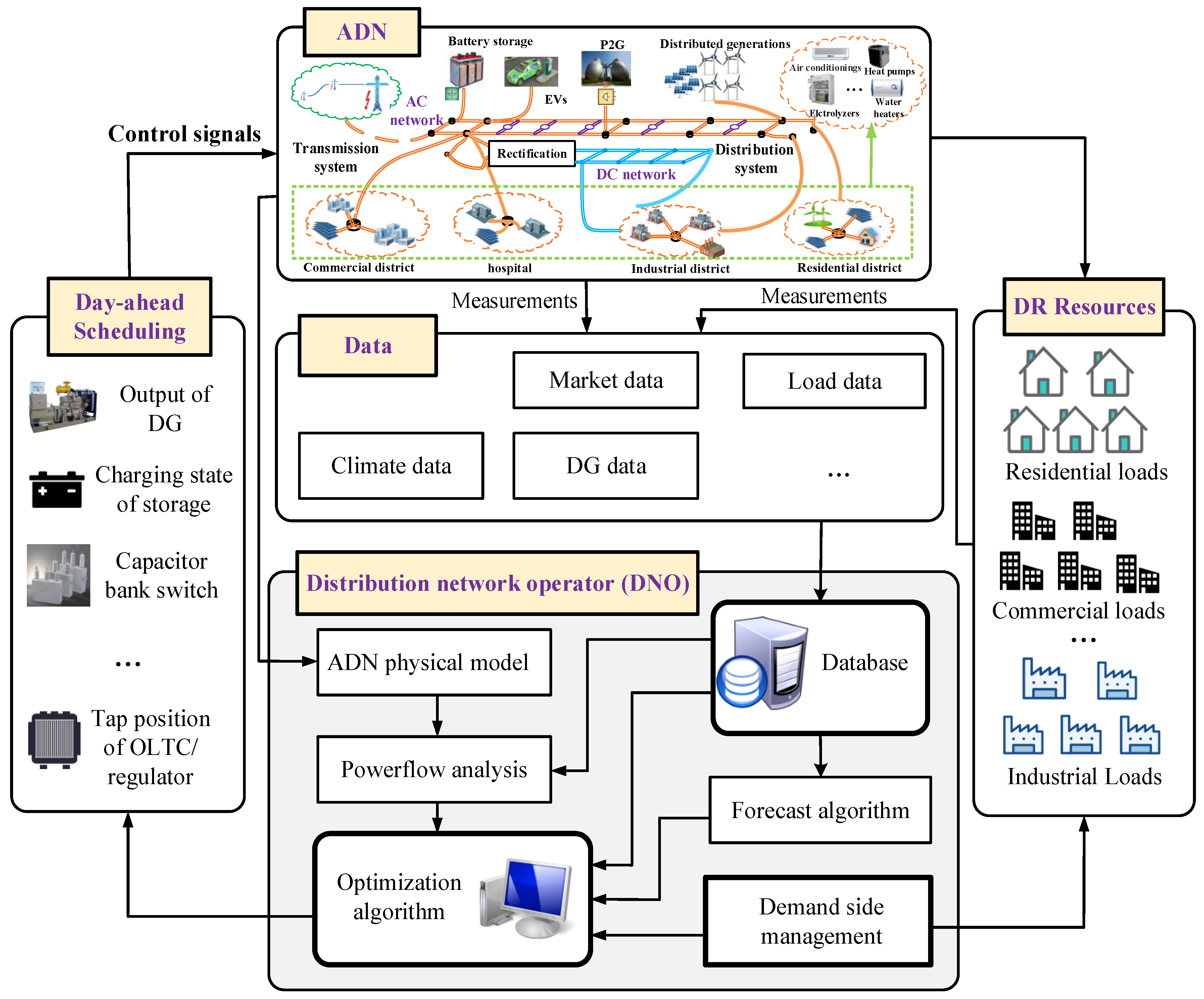
2. Problem Formulation
2.1. Objective Function
2.2. Constraints
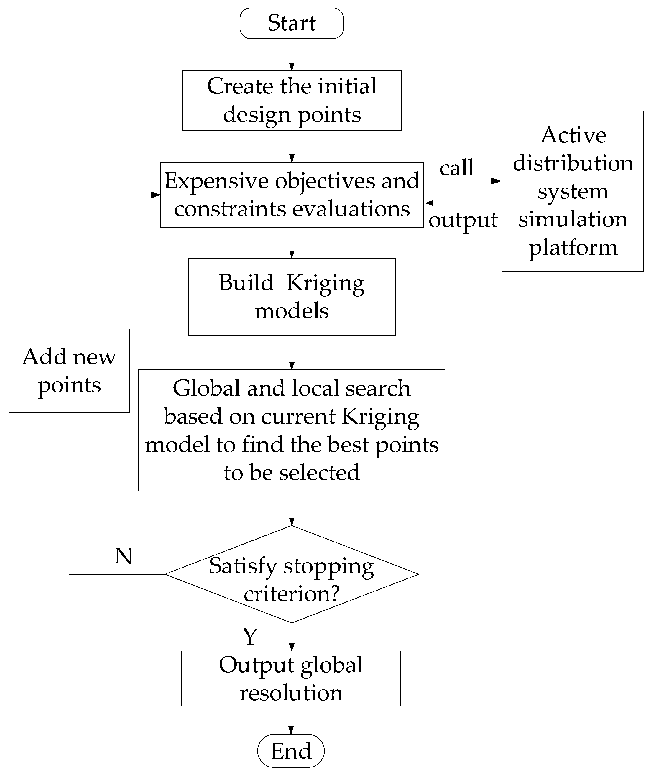
3. Model Solution
3.1. Kriging Model
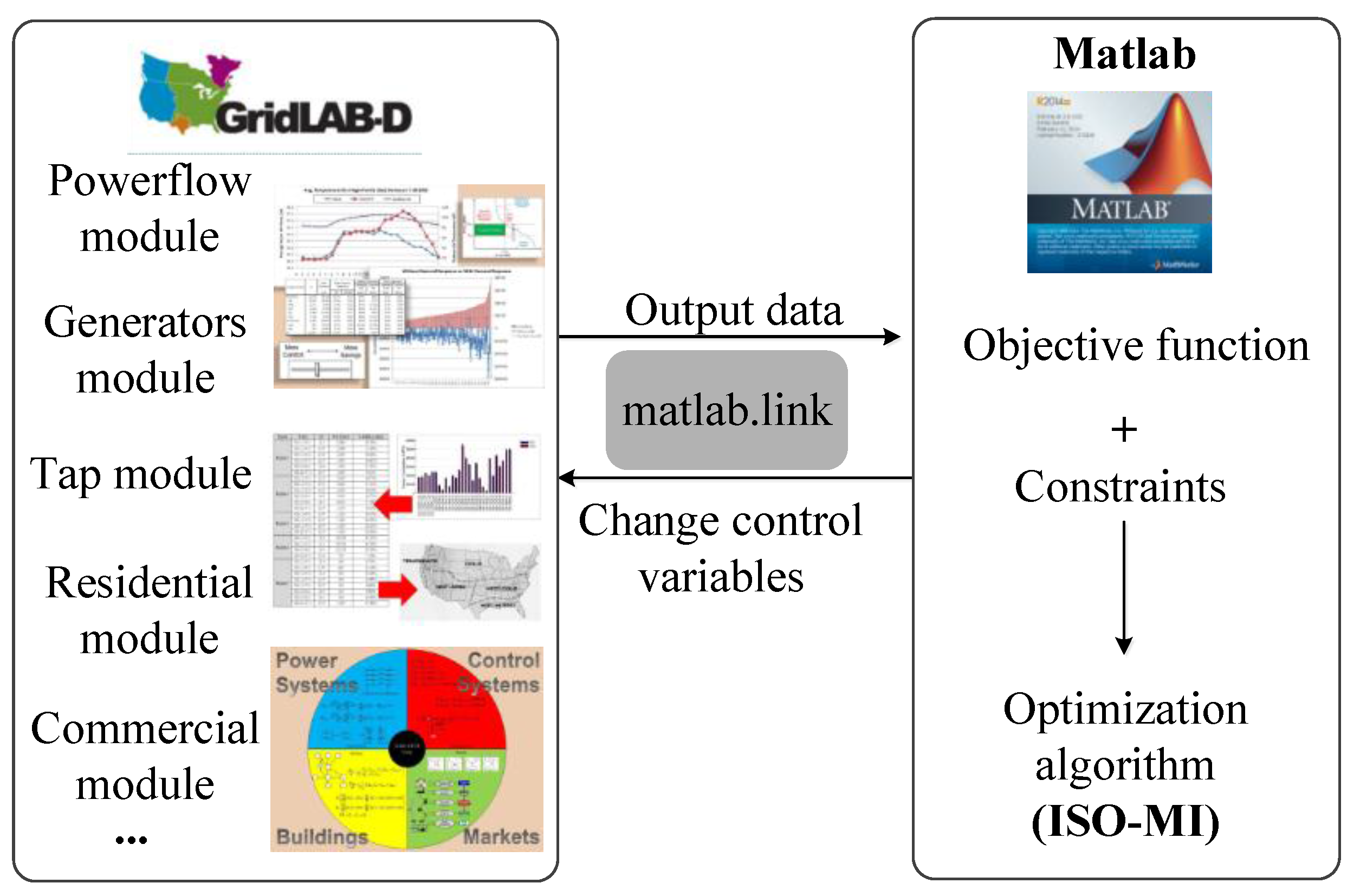
3.2. Kriging Model Based Optimization
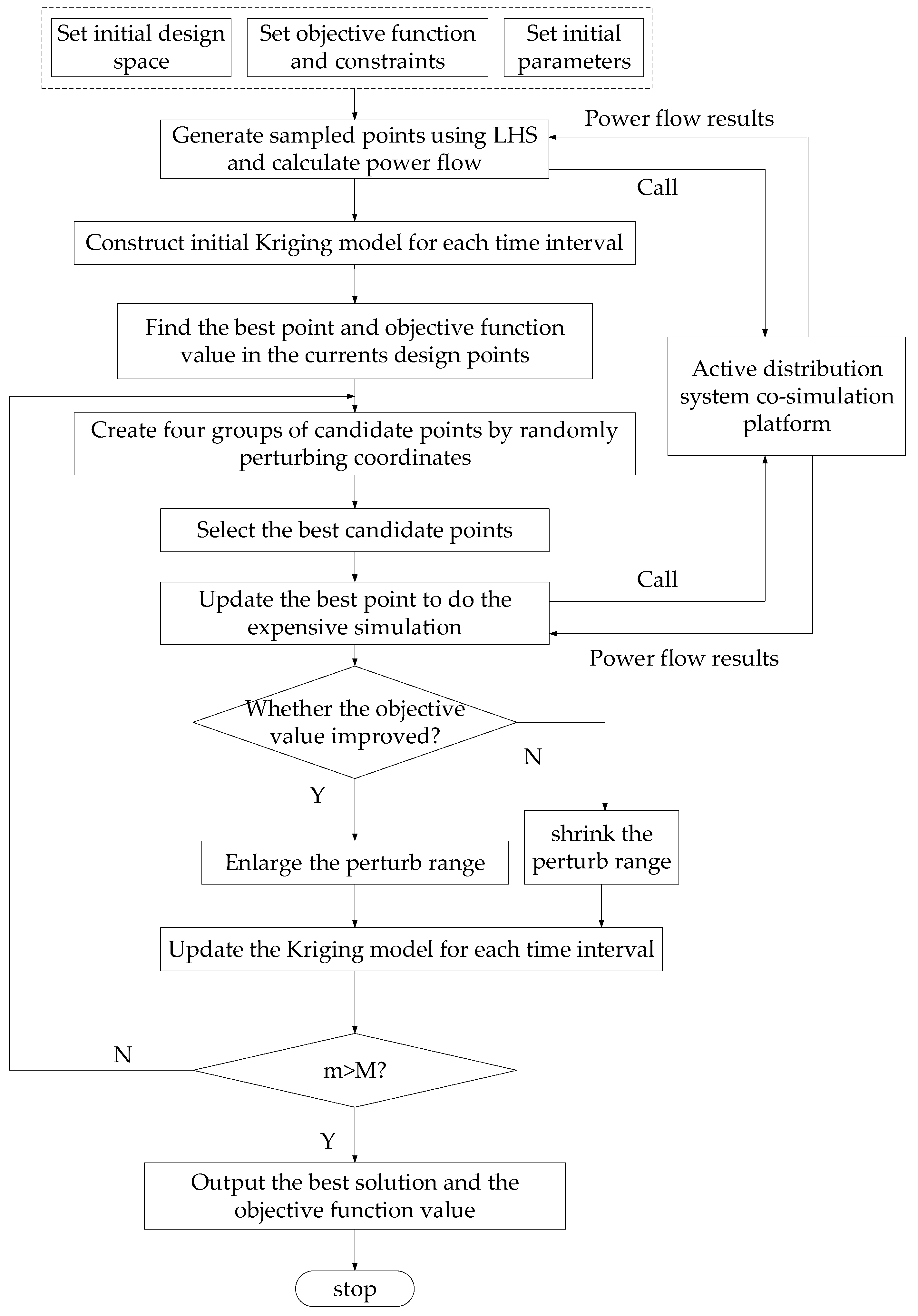
3.3. Improved Surrogate Optimization-Mixed-Integer Algorithm
- (1)
- Group 1: Uniformly and randomly perturb the continuous coordinates of at the range of , , where i is the index of points and ;
- (2)
- Group 2: Uniformly and randomly perturb the discrete coordinates of at the range of , ;
- (3)
- Group 3: Uniformly and randomly perturb all coordinates of at the range of , and round the discrete coordinates to the closet integers;
- (4)
- Group 4: Select candidate points in the whole design space using LHS.
- (1)
- Calculate the objective function using the initial Kriging model and current new Kriging model of candidate points in four groups and compute the objective function score and of all points, where and are the normalized objective functions. Their value can be calculated by Euclidean distance in n dimensional space.
- (2)
- Compute the distance score of all design points.
- (3)
- Compute the weighted score , where denotes the objective function F in this paper, and select the point with minimum score to add it into design points set and do the expensive function evaluation, again.
4. Simulation and Case Studies
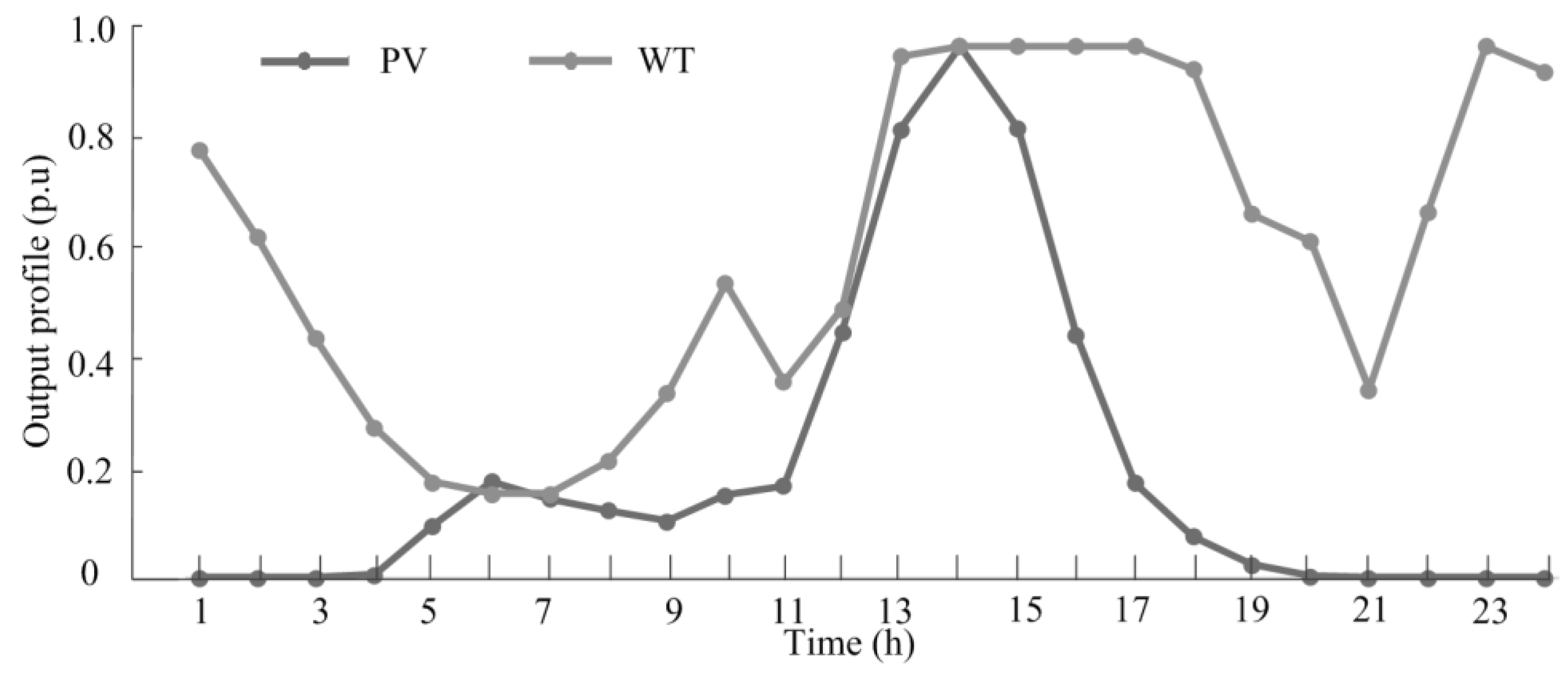
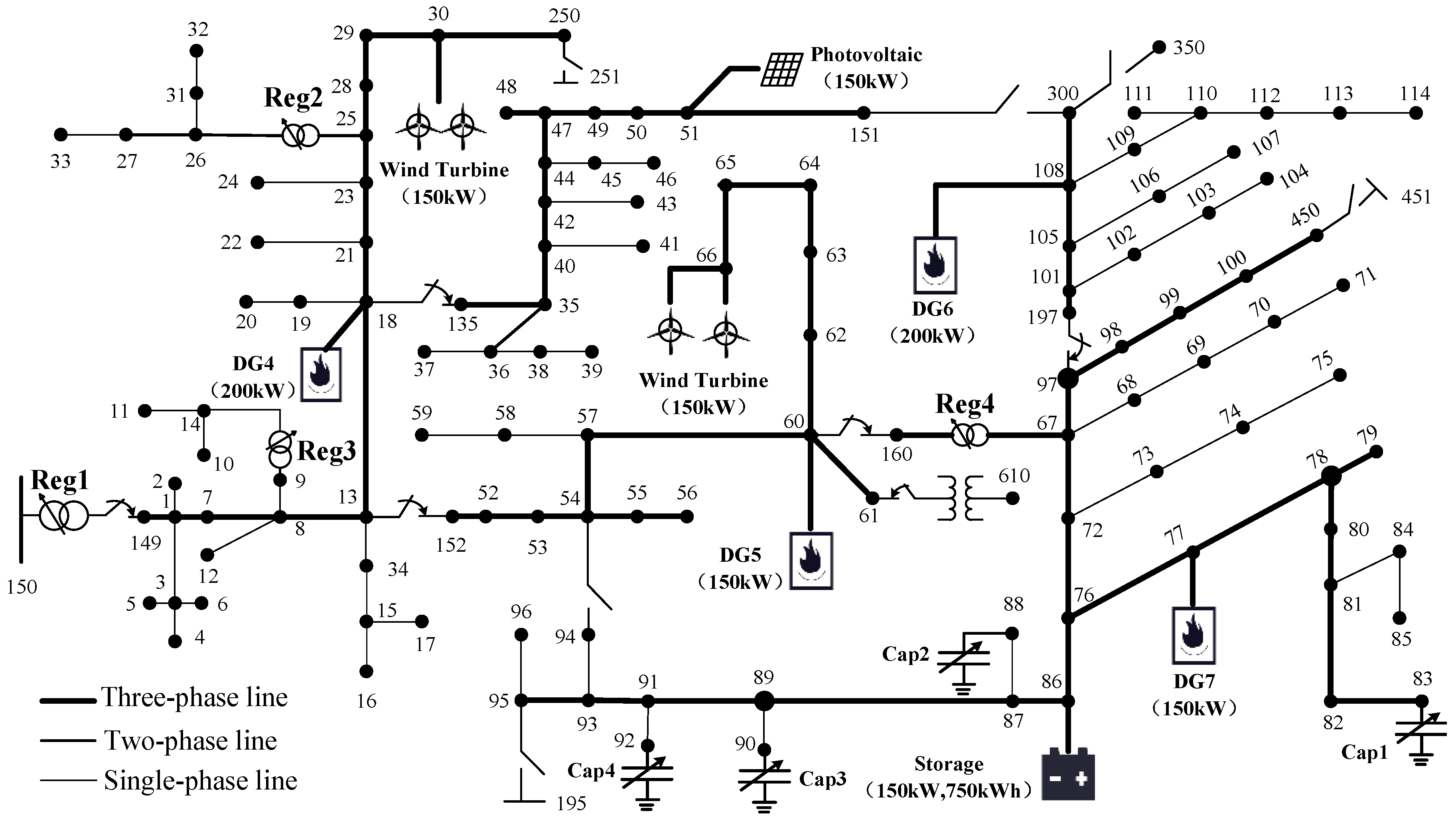
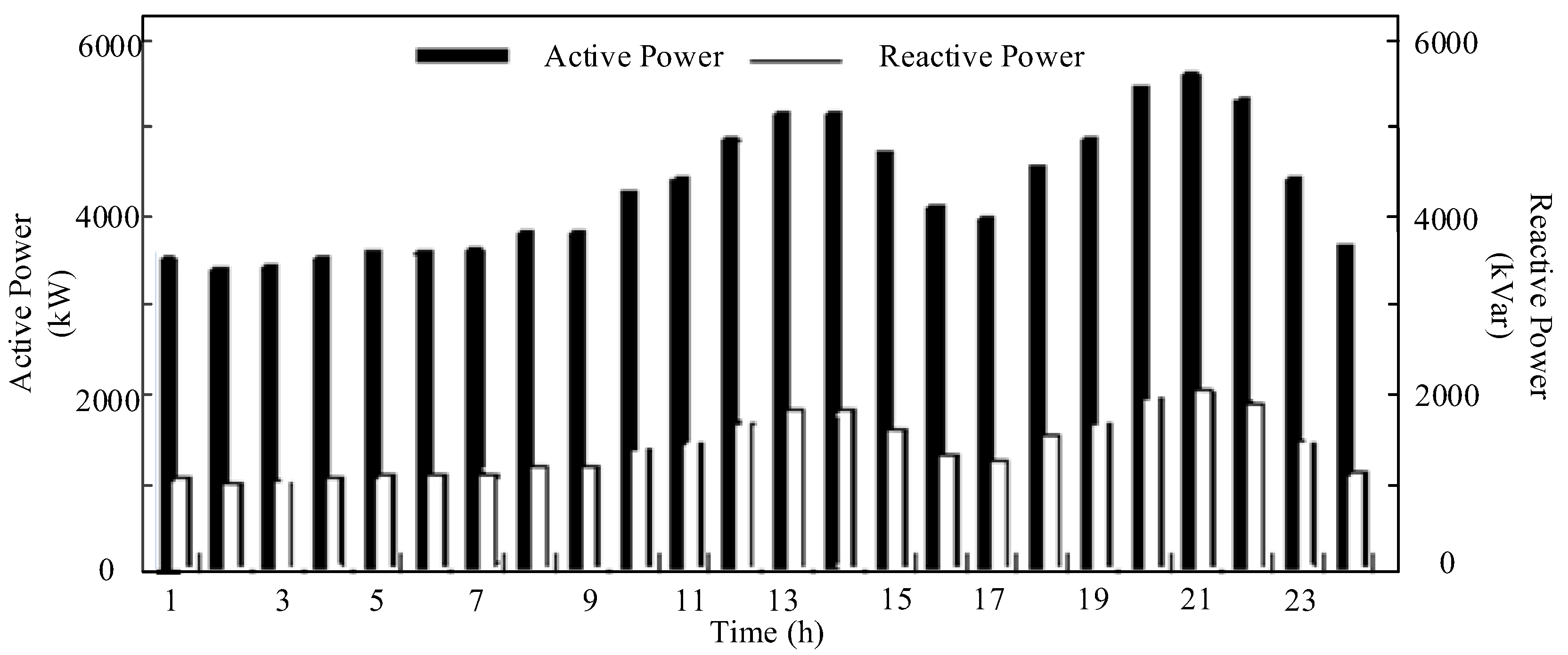
4.1. Test System Specification
4.2. Accuracy of Kriging Model in Distribution System
- (1)
- Root Mean Square Error (RMSE):
- (2)
- Relative Maximum Absolute Error (RMAX):
- (3)
- Relative Average Absolute Error (RAAE):
- (4)
- R-Square:
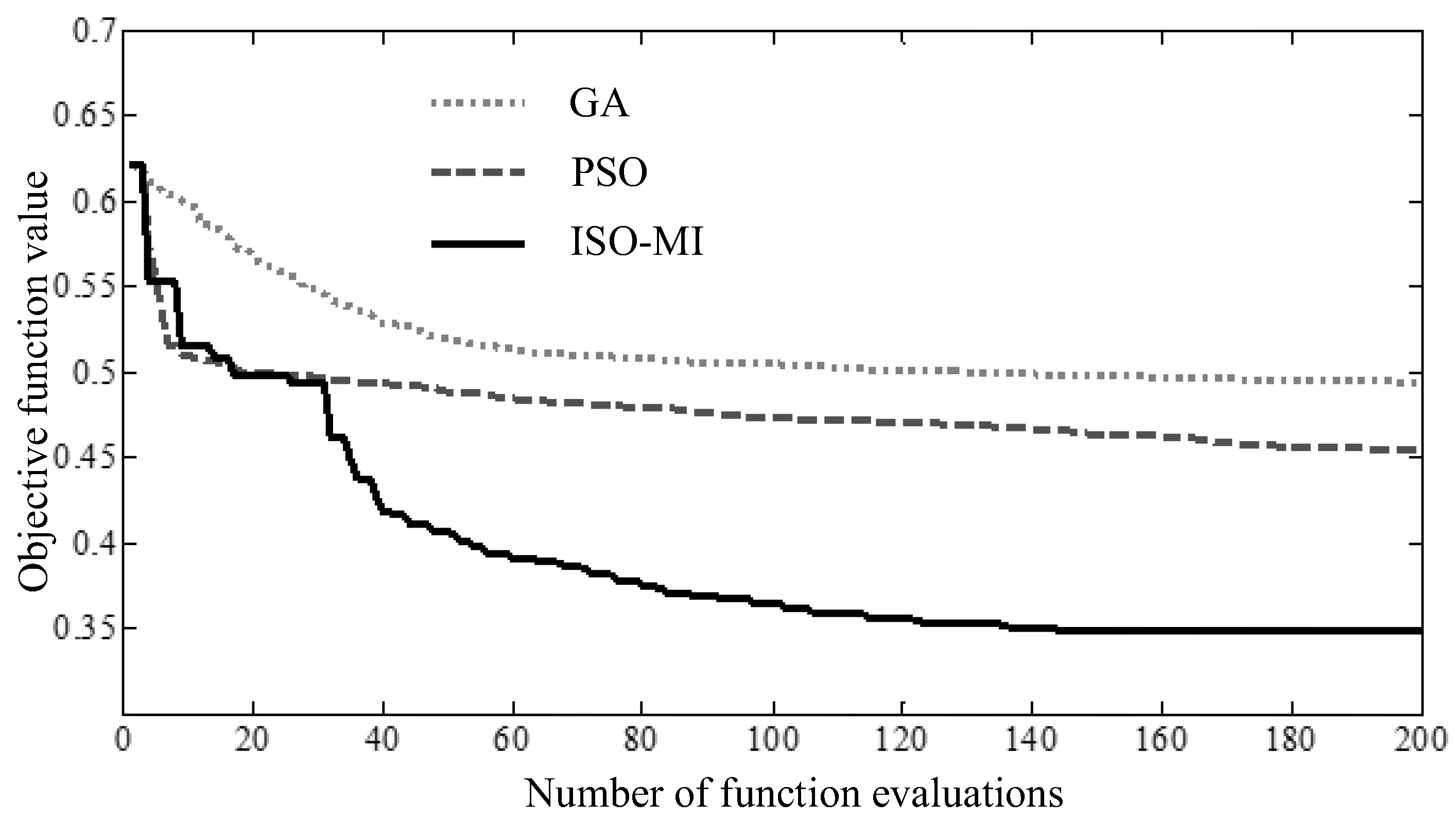
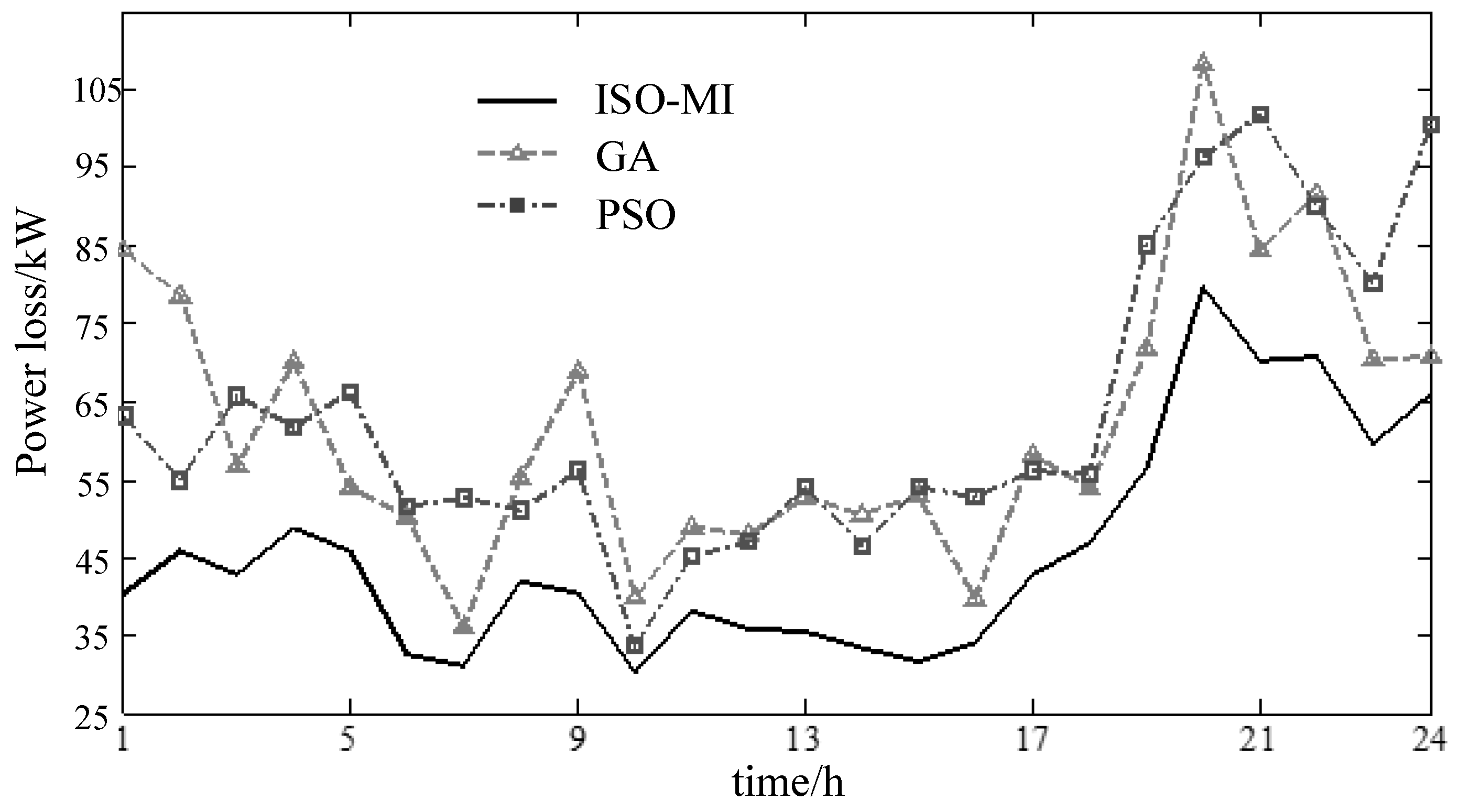
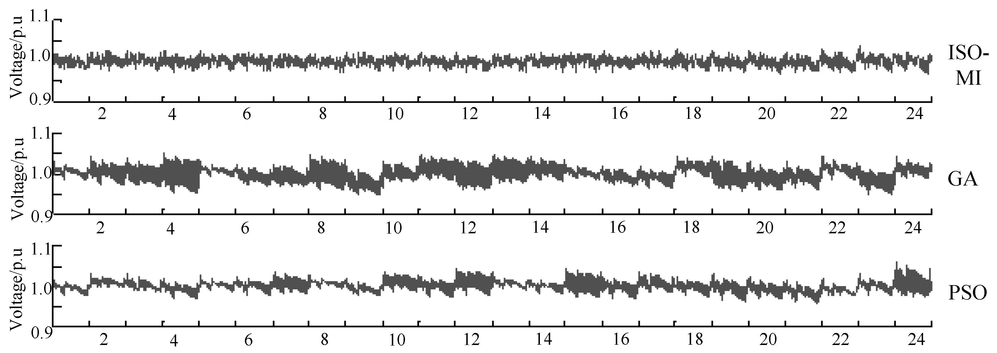
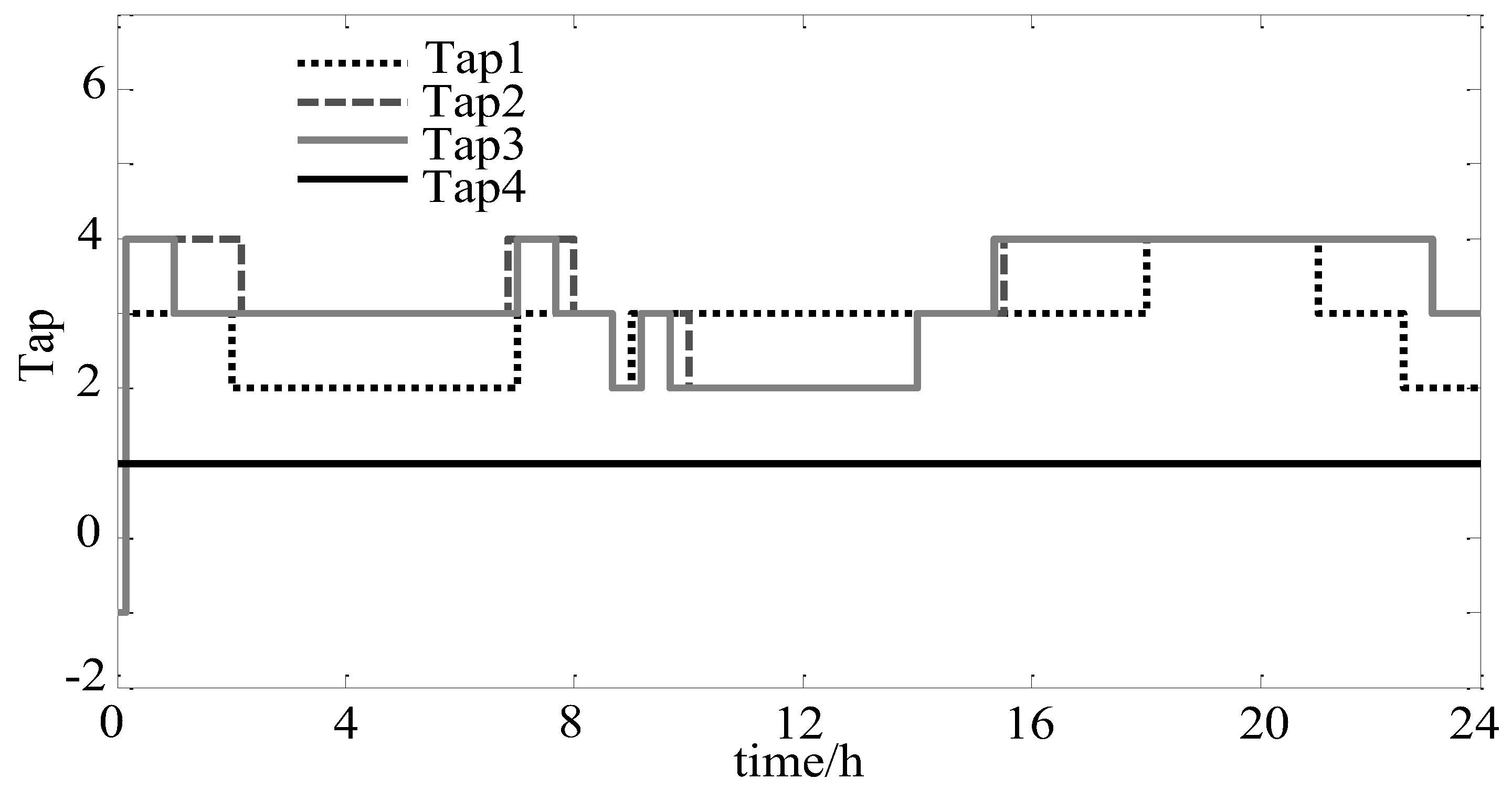
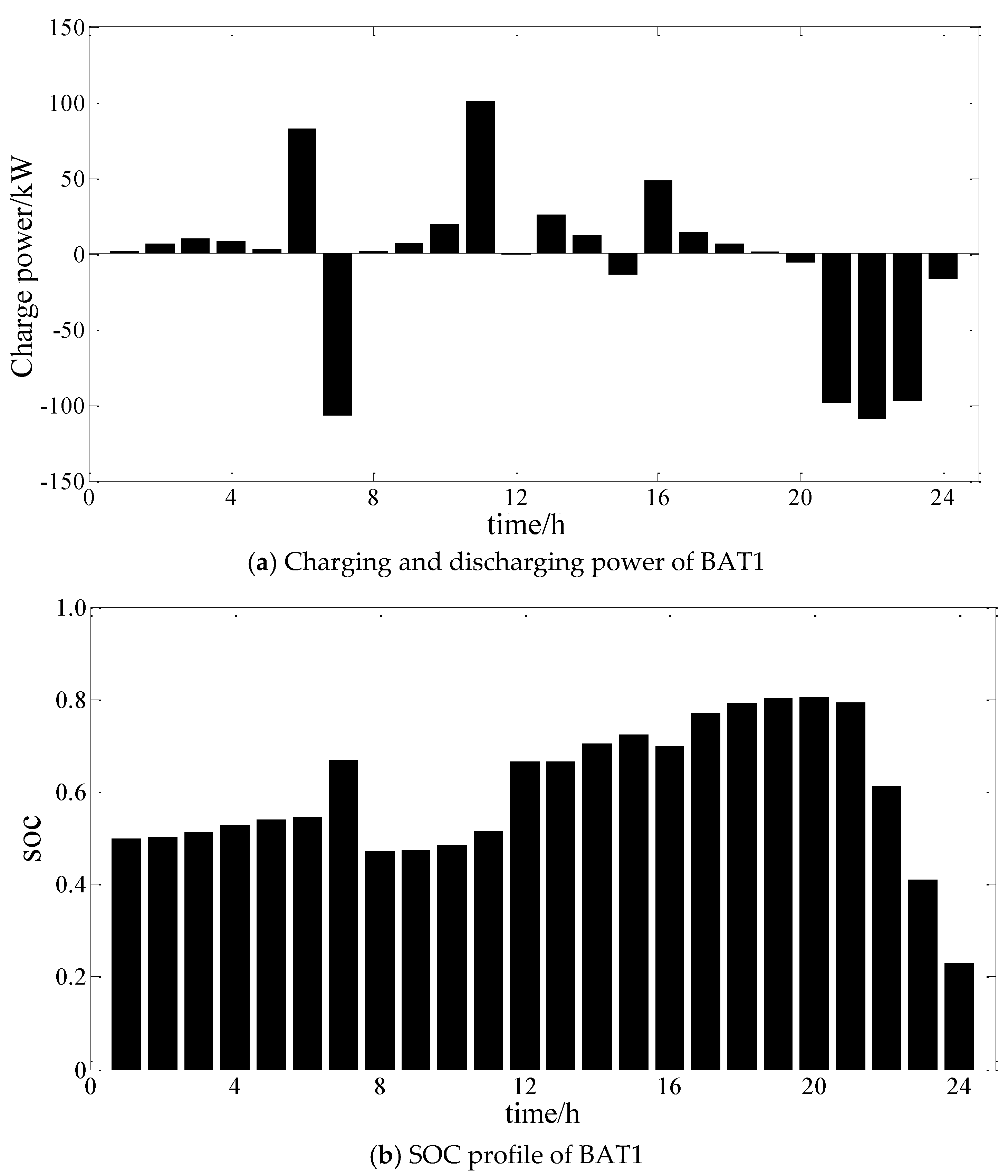
4.3. Solving Efficiency of ISO-MI
5. Conclusions
Acknowledgments
Author Contributions
Conflicts of Interest
References
- Atwa, Y.M.; El-Saadany, E.F.; Salama, M.M.A. Optimal renewable resources mix for distribution system energy loss minimization. IEEE Trans. Power Syst. 2010, 25, 360–370. [Google Scholar] [CrossRef]
- Huang, A.Q.; Crow, M.L.; Heydt, G.T. The future renewable electric energy delivery and management (FREEDM) system: The energy internet. Proc. IEEE 2011, 99, 133–148. [Google Scholar] [CrossRef]
- Zhao, B.; Wang, C.; Zhou, J.; Zhao, J.; Yang, Y.; Yu, J. Present and Future Development Trend of Active Distribution Network. Autom. Electr. Power Syst. 2014, 38, 125–135. [Google Scholar]
- Yi, Y.; Liu, D.; Yu, W.; Chen, F.; Pan, F. Technology and Its Trends of Active Distribution Network. Autom. Electr. Power Syst. 2012, 36, 10–16. [Google Scholar]
- Farhangi, H. The path of the smart grid. IEEE Power Energy Mag. 2010, 8, 18–28. [Google Scholar] [CrossRef]
- Senjyu, T.; Miyazato, Y.; Yona, A. Optimal distribution voltage control and coordination with distributed generation. IEEE Trans. Power Deliv. 2008, 23, 1236–1242. [Google Scholar] [CrossRef]
- Manbachi, M.; Farhangi, H.; Palizban, A. A novel Volt-VAR Optimization engine for smart distribution networks utilizing Vehicle to Grid dispatch. Int. J. Electr. Power Energy Syst. 2016, 74, 238–251. [Google Scholar] [CrossRef]
- Ahmadi, H.; Martí, J.R.; Dommel, H.W. A framework for volt-VAR optimization in distribution systems. IEEE Trans. Smart Grid 2015, 6, 1473–1483. [Google Scholar] [CrossRef]
- Padilha-Feltrin, A.; Quijano Rodezno, D.A.; Sanches Mantovani, J.R. Volt-VAR Multiobjective Optimization to Peak-Load Relief and Energy Efficiency in Distribution Networks. IEEE Trans. Power Deliv. 2015, 30, 618–626. [Google Scholar] [CrossRef]
- Manbachi, M.; Sadu, A.; Farhangi, H. Impact of EV penetration on Volt-VAR optimization of distribution networks using real-time co-simulation monitoring platform. Appl. Energy 2016, 169, 28–39. [Google Scholar] [CrossRef]
- Niknam, T.; Firouzi, B.B.; Ostadi, A. A new fuzzy adaptive particle swarm optimization for daily Volt/Var control in distribution networks considering distributed generators. Appl. Energy 2010, 87, 1919–1928. [Google Scholar] [CrossRef]
- Sousa, T.; Morais, H.; Soares, J.; Vale, Z. Day-ahead resource scheduling in smart grids considering Vehicle-to-Grid and network constraints. Appl. Energy 2012, 96, 183–193. [Google Scholar] [CrossRef]
- Wu, H.; Liu, X.; Ding, M. Dynamic economic dispatch of a microgrid: Mathematical models and solution algorithm. Int. J. Electr. Power Energy Syst. 2014, 63, 336–346. [Google Scholar] [CrossRef]
- Ippolito, M.G.; Silvestre, M.L.D.; Sanseverino, E.R. Multi-objective optimized management of electrical energy storage systems in an islanded network with renewable energy sources under different design scenarios. Energy 2014, 64, 648–662. [Google Scholar] [CrossRef]
- Di Silvestre, M.L.; La Cascia, D.; Sanseverino, E.R. Improving the energy efficiency of an islanded distribution network using classical and innovative computation methods. Utilities Policy 2016, 40, 58–66. [Google Scholar] [CrossRef]
- Wu, H.; Shahidehpour, M.; Alabdulwahab, A. Demand response exchange in the stochastic day-ahead scheduling with variable renewable generation. IEEE Trans. Sustain. Energy 2015, 6, 516–525. [Google Scholar] [CrossRef]
- Mazidi, M.; Monsef, H.; Siano, P. Robust day-ahead scheduling of smart distribution networks considering demand response programs. Appl. Energy 2016, 178, 929–942. [Google Scholar] [CrossRef]
- Rao, R.S.; Ravindra, K.; Satish, K. Power loss minimization in distribution system using network reconfiguration in the presence of distributed generation. IEEE Trans. Power Syst. 2013, 28, 317–325. [Google Scholar] [CrossRef]
- Kayal, P.; Chanda, C.K. Placement of wind and solar based DGs in distribution system for power loss minimization and voltage stability improvement. Int. J. Electr. Power Energy Syst. 2013, 53, 795–809. [Google Scholar] [CrossRef]
- Estevam, C.R.N.; Rider, M.J.; Amorim, E. Reactive power dispatch and planning using a non-linear branch-and-bound algorithm. IET Gener. Transm. Distrib. 2010, 4, 963–973. [Google Scholar] [CrossRef]
- Khodr, H.M.; Martinez-Crespo, J.; Matos, M.A. Distribution systems reconfiguration based on OPF using Benders decomposition. IEEE Trans. Power Deliv. 2009, 24, 2166–2176. [Google Scholar] [CrossRef]
- Ghasemi, A.; Mortazavi, S.S.; Mashhour, E. Hourly demand response and battery energy storage for imbalance reduction of smart distribution company embedded with electric vehicles and wind farms. Renew. Energy 2016, 85, 124–136. [Google Scholar] [CrossRef]
- Wang, X.; Palazoglu, A.; El-Farra, N.H. Operational optimization and demand response of hybrid renewable energy systems. Appl. Energy 2015, 143, 324–335. [Google Scholar] [CrossRef]
- Manbachi, M.; Farhangi, H.; Palizban, A. Smart grid adaptive energy conservation and optimization engine utilizing particle swarm optimization and fuzzification. Appl. Energy 2016, 174, 69–79. [Google Scholar] [CrossRef]
- Niknam, T.; Mojarrad, H.D.; Meymand, H.Z. A new honey bee mating optimization algorithm for non-smooth economic dispatch. Fuel Energy Abstr. 2011, 36, 896–908. [Google Scholar] [CrossRef]
- Christakou, K.; Paolone, M.; Abur, A. Voltage Control in Active Distribution Networks under Uncertainty in the System Model: A Robust Optimization Approach. IEEE Trans. Smart Grid 2017. [CrossRef]
- Zhao, J.; Xu, L.; Lin, C.; Wei, W. Three-phase Unbalanced Reactive Power Optimization for Distribution Systems with a Large Number of Single Phase Solar Generators. Autom. Electr. Power Syst. 2016, 40, 13–18. [Google Scholar]
- Wand, X.; Lv, Z.; Yang, Z. Dynamic dispatching for microgrid with storage battery charging-discharging times constraint based on improved GA. J. Guangxi Univ. (Nat. Sci. Ed.) 2017, 42, 560–570. [Google Scholar]
- Yang, Y.; Pei, W.; Deng, W.; Shen, Z.; Qi, Z.; Zhou, M. Day-Ahead Scheduling Optimization for Microgrid with Battery Life Model. Trans. China Electrotech. Soc. 2015. [CrossRef]
- Booker, A.J.; Dennis, J.E.; Frank, P.D. A rigorous framework for optimization of expensive functions by surrogates. Struct. Multidiscip. Optim. 1998, 17, 1–13. [Google Scholar] [CrossRef]
- Davis, E.; Ierapetritou, M. A kriging based method for the solution of mixed-integer nonlinear programs containing black-box functions. J. Glob. Optim. 2009, 43, 191–205. [Google Scholar] [CrossRef]
- Kim, B.S.; Lee, Y.B.; Choi, D.H. Comparison study on the accuracy of metamodeling technique for non-convex functions. J. Mech. Sci. Technol. 2009, 23, 1175–1181. [Google Scholar] [CrossRef]
- Simpson, T.W.; Poplinski, J.D.; Koch, P.N. Metamodels for computer-based engineering design: Survey and recommendations. Eng. Comput. 2001, 17, 129–150. [Google Scholar] [CrossRef]
- Xuan, Y.; Xiang, J.H.; Zhang, W.H.; Zhang, Y.L. Gradient-based Kriging approximate model and its application research to optimization design. Chin. Sci. Tech. Sci. 2009, 52, 1117–1124. [Google Scholar] [CrossRef]
- Simpson, T.W.; Mauery, T.M.; Korte, J.J. Kriging models for global approximation in simulation-based multidisciplinary design optimization. AIAA J. 2015, 39, 2233–2241. [Google Scholar] [CrossRef]
- Lophaven, S.N.; Nielsen, H.B.; Sondergaard, J. DACE: A Matlab Kriging Toolbox, Version 2.0; Technical Report; IMM Technical University of Denmark: Lyngby, Denmark, 2002. [Google Scholar]
- Younis, A.A.H. Space Exploration and Region Elimination Global Optimization Algorithms for Multidisciplinary Design Optimization. Available online: http://dspace.library.uvic.ca/bitstream/handle/1828/3325/Adel%20Younis_%20PhD%20Dissertation_Mechanical%20Engineering_%202010-8.pdf?sequence=1&isAllowed=y (accessed on 15 December 2017).
- Petelet, M.; Iooss, B.; Asserin, O.; Loredo, A. Latin hypercube sampling with inequality constraints. AStA Adv. Stat. Anal. 2010, 94, 325–339. [Google Scholar] [CrossRef]
- Müller, J. MISO: Mixed-integer surrogate optimization framework. Optim. Eng. 2016, 17, 177–203. [Google Scholar] [CrossRef]
- Müller, J.; Shoemaker, C.A.; Piché, R. SO-MI: A surrogate model algorithm for computationally expensive nonlinear mixed-integer black-box global optimization problems. Comput. Oper. Res. 2013, 40, 1383–1400. [Google Scholar] [CrossRef]
- Regis, R.G.; Shoemaker, C.A. Combining radial basis function surrogates and dynamic coordinate search in high-dimensional expensive black-box optimization. Eng. Optim. 2012, 45, 1–27. [Google Scholar] [CrossRef]
- Chassin, D.P.; Fuller, J.C.; Djilali, N. GridLAB-D: An agent-based simulation framework for smart grids. J. Appl. Math. 2014, 2014, 492320. [Google Scholar] [CrossRef]
- Chassin, D.P.; Schneider, K.; Gerkensmeyer, C. GridLAB-D: An open-source power system modeling and simulation environment. In Proceedings of the IEEE Transmission and Distribution Conference and Exposition, Chicago, IL, USA, 21–24 April 2008; pp. 1–5. [Google Scholar]
- Tang, J.; Wang, D.; Wang, X.; Jia, H.; Wang, C.; Huang, R.; Yangd, Z.; Fan, M. Study on day-ahead optimal economic operation of active distribution networks based on Kriging model assisted particle swarm optimization with constraint handling techniques. Appl. Energy 2017, 204, 143–162. [Google Scholar] [CrossRef]
- Distribution System Analysis Subcommittee. Available online: http://ewh.ieee.org/soc/pes/dsacom/testfeeders/ (accessed on 15 December 2017).
- Bokhari, A.; Alkan, A.; Dogan, R.; Diaz-Aguiló, M.; de León, F.; Czarkowski, D.; Zabar, Z.; Birenbaum, L.; Noel, A.; Uosef, R.E. Experimental Determination of the ZIP Coefficients for Modern Residential, Commercial, and Industrial Loads. IEEE Trans. Power Deliv. 2014, 29, 1372–1381. [Google Scholar] [CrossRef]
- Dyn, N.; Levin, D.; Rippa, S. Numerical Procedures for Surface Fitting of Scattered Data by Radial Basis Functions. SIAM J. Sci. Stat. Comput. 1986, 7, 639–659. [Google Scholar] [CrossRef]
- Jin, R.; Chen, W.; Simpson, T. Comparative studies of metamodeling techniques under multiple modeling criteria. In Proceedings of the 8th Symposium on Multidisciplinary Analysis and Optimization (AIAA), Long Beach, CA, USA, 6–8 September 2000. [Google Scholar]


| Name | Installed Location | Phases | Tap Range | Voltage Regulation Range | Maximum Operating Times |
|---|---|---|---|---|---|
| Reg1 | 150–149 | A-B-C | [−16, +16] | [0.95, 1.05] | 10 |
| Reg1 | 25–26 | A-C | [−16, +16] | [0.95, 1.05] | 10 |
| Reg1 | 9–14 | A | [−16, +16] | [0.95, 1.05] | 10 |
| Reg1 | 160–67 | A-B-C | [−16, +16] | [0.95, 1.05] | 10 |
| Name | Installed Location | Installed Capacity (kVar) | Maximum Operating Times | ||
|---|---|---|---|---|---|
| Phase A | Phase B | Phase C | |||
| Cap1 | 83 | 100 | 100 | 100 | 10 |
| Cap2 | 88 | 50 | 0 | 0 | 10 |
| Cap3 | 90 | 0 | 50 | 0 | 10 |
| Cap4 | 92 | 0 | 0 | 50 | 10 |
| Name | Installed Location | Type | Rated Power (kW) | Power Factor |
|---|---|---|---|---|
| DG1 | 66 | WT | 150 | 0.9 |
| DG1 | 51 | PV | 100 | 0.9 |
| DG1 | 30 | MT | 150 | 0.9 |
| DG1 | 18 | MT | 200 | 0.9–1.0 |
| DG1 | 60 | MT | 150 | 0.9–1.0 |
| DG1 | 108 | MT | 200 | 0.9–1.0 |
| DG1 | 77 | MT | 150 | 0.9–1.0 |
| ZIP Coefficients | Z | I | P |
|---|---|---|---|
| Active load | 0.418 | 0.135 | 0.447 |
| Reactive load | 0.515 | 0.023 | 0.462 |
| Name | Installed Location | Power (kW) | Capacity (kWh) | Efficiency | |
|---|---|---|---|---|---|
| Charging | Discharging | ||||
| BAT1 | 86 | [–150, 150] | 750 | 0.9 | 0.9 |
| N | 50 | 100 | 200 | |
|---|---|---|---|---|
| Index | ||||
| Voltage fluctuation | RMSE | 9.4 × 10⁻⁵ | 9.0 × 10⁻⁵ | 9.1 × 10⁻⁵ |
| RMAE | 7.5 × 10⁻⁴ | 7.2 × 10⁻⁴ | 6.2 × 10⁻⁴ | |
| RAAE | 6.3 × 10⁻⁵ | 5.9 × 10⁻⁵ | 5.2 × 10⁻⁵ | |
| R2 | 1.0000 | 1.0000 | 1.0000 | |
| Power loss | RMSE | 2.3 × 10⁻³ | 1.9 × 10⁻³ | 1.3 × 10⁻³ |
| RMAE | 3.4 × 10⁻³ | 2.5 × 10⁻³ | 1.9 × 10⁻³ | |
| RAAE | 1.1 × 10⁻³ | 0.9 × 10⁻³ | 0.7 × 10⁻³ | |
| R2 | 0.9954 | 0.9973 | 0.9988 | |
© 2017 by the authors. Licensee MDPI, Basel, Switzerland. This article is an open access article distributed under the terms and conditions of the Creative Commons Attribution (CC BY) license (http://creativecommons.org/licenses/by/4.0/).
Share and Cite
Wang, D.; Hu, Q.; Tang, J.; Jia, H.; Li, Y.; Gao, S.; Fan, M. A Kriging Model Based Optimization of Active Distribution Networks Considering Loss Reduction and Voltage Profile Improvement. Energies 2017, 10, 2162. https://doi.org/10.3390/en10122162
Wang D, Hu Q, Tang J, Jia H, Li Y, Gao S, Fan M. A Kriging Model Based Optimization of Active Distribution Networks Considering Loss Reduction and Voltage Profile Improvement. Energies. 2017; 10(12):2162. https://doi.org/10.3390/en10122162
Chicago/Turabian StyleWang, Dan, Qing’e Hu, Jia Tang, Hongjie Jia, Yun Li, Shuang Gao, and Menghua Fan. 2017. "A Kriging Model Based Optimization of Active Distribution Networks Considering Loss Reduction and Voltage Profile Improvement" Energies 10, no. 12: 2162. https://doi.org/10.3390/en10122162
APA StyleWang, D., Hu, Q., Tang, J., Jia, H., Li, Y., Gao, S., & Fan, M. (2017). A Kriging Model Based Optimization of Active Distribution Networks Considering Loss Reduction and Voltage Profile Improvement. Energies, 10(12), 2162. https://doi.org/10.3390/en10122162