Article

Stochastic Dynamic AC Optimal Power Flow Based on a Multivariate Short-Term Wind Power Scenario Forecasting Model

1
Energy Management System, ABB Enterprise Software, Sugar Land, TX 77478, USA
2
Electrical Engineering, Konkuk University, Seoul 05029, Korea
3
Department of Electrical & Computer Engineering , Baylor University, Waco, TX 76798, USA
*
Author to whom correspondence should be addressed.
Energies 2017, 10(12), 2138; https://doi.org/10.3390/en10122138
Submission received: 21 November 2017 / Revised: 9 December 2017 / Accepted: 11 December 2017 / Published: 15 December 2017
(This article belongs to the Section F: Electrical Engineering)

Abstract

:
The deterministic methods generally used to solve DC optimal power flow (OPF) do not fully capture the uncertainty information in wind power, and thus their solutions could be suboptimal. However, the stochastic dynamic AC OPF problem can be used to find an optimal solution by fully capturing the uncertainty information of wind power. That uncertainty information of future wind power can be well represented by the short-term future wind power scenarios that are forecasted using the generalized dynamic factor model (GDFM)—a novel multivariate statistical wind power forecasting model. Furthermore, the GDFM can accurately represent the spatial and temporal correlations among wind farms through the multivariate stochastic process. Fully capturing the uncertainty information in the spatially and temporally correlated GDFM scenarios can lead to a better AC OPF solution under a high penetration level of wind power. Since the GDFM is a factor analysis based model, the computational time can also be reduced. In order to further reduce the computational time, a modified artificial bee colony (ABC) algorithm is used to solve the AC OPF problem based on the GDFM forecasting scenarios. Using the modified ABC algorithm based on the GDFM forecasting scenarios has resulted in better AC OPF’ solutions on an IEEE 118-bus system at every hour for 24 h.

1. Introduction

With the increasing penetration level of wind power, challenges from the variability and uncertainty, more precisely from the stochasticity of wind power [1,2], of wind power to power system reliability have been reported by researchers and system operators [3]. One way to mitigate the effect of variability and uncertainty of wind power on the optimal power flow (OPF) is to solve the stochastic dynamic ACOPF problem by considering many possible wind power forecasting scenarios, which are generally synthesized using Monte Carlo simulation [4]. However, this approach has certain drawbacks, such as a high computational burden and the difficulty of generating accurate scenarios. Recently, as new wind power scenario forecasting techniques and fast stochastic optimization algorithms have been developed, researchers and system operators have studied the stochastic dynamic AC OPF [5].
Wind power forecasting has two major approaches in terms of output: point forecasting and probabilistic forecasting. Point forecasting gives a single future wind power output. On the contrary, probabilistic forecasting gives a conditional distribution of future wind power output [6], so that system operators and traders can utilize a much broader set of information. The wind power distribution can be represented as quantiles, interval forecasts, probability density functions (PDFs) and scenarios.
Extensive research on probabilistic wind power forecasting has been conducted [7]. Monteiro et al. in [8] gave a comprehensive review of methodologies for probabilistic wind power forecasting, which includes physical models, statistical models, and combined models. A traditional, physical time-series model, such as the autoregressive model (AR), captures the temporal correlation in wind. This model predicts the distribution of future wind power as a linear combination of previous and current data and white noise errors [9]. A statistical space-time model was proposed in [10]. It considered the terrain, wind direction and wind speed as the input data.
However, few of the previously mentioned works have focused on the stochastic process with multiple wind farms even though the spatial correlation among wind farms has played an important role for the reliability of the power system. For example, wind farms that have a positive spatial correlation and share the same transmission lines might congest the transmission lines, and the transmission congestion could curtail the electricity supply [11].
A model that can consider the spatial and temporal correlation among variables is called a spatio-temporal model. Among many spatio-temporal models, the generalized dynamic factor model (GDFM) was used to generate wind power and load scenarios for transmission expansion planning [12]. The GDFM can address the spatial and temporal correlation among wind farms in nearby areas where wind power is affected by similar weather conditions, transmission lines and movements over time.
In this work, we extend this previous GDFM to forecast the short-term probabilistic wind power and represent the distribution of wind power forecasts as multiple wind power scenarios. The future wind power forecasting scenarios for 24 h are forecasted to solve the stochastic dynamic AC OPF problem.
The forecasted wind power scenarios can be used in stochastic optimization. The advantage of stochastic optimization based on the forecasted wind power scenarios is that system operators can find the optimal expected benefits by fully capturing the uncertainty information of wind power. Scenario-based stochastic programming and chance-constrained methods are common approaches for stochastic optimization with wind power. For instance, Wang et al. [13] proposed a stochastic security unit commitment by integrating the intermittency of wind power to generate the scenarios using Monte Carlo (MC) simulation. The computational cost is very high because the MC simulation does not consider the correlations among scenarios, and therefore an extensive number of scenarios needs to be generated in order to fully represent combinations of various wind farms.
In this study, instead of the simplified DC OPF model, we then implement the AC OPF model in the stochastic optimization in order to find more accurate solutions. The solutions include real power outputs, reactive power outputs, bus voltages and bus angles. Furthermore, the dynamic OPF is an extended OPF dispatching optimal power flows over multiple time periods. Here, we propose the stochastic dynamic AC OPF to calculate the optimal dispatch by incorporating the variability and uncertainty of wind power based on wind power forecasting scenarios over 24 h and considering the correlation among scenarios. The GDFM is able to maintain the spatial and temporal correlation among scenarios. On the contrary, the MC simulation generates uncorrelated random forecast scenarios based on the predefined multivariate probability density function (PDF).
The stochastic dynamic AC OPF is a mixed-integer, nonlinear programming (MINLP) problem with high non-linearity and non-convexity, which requires a robust and feasible methodology. Unfortunately, traditional mathematical tools are very inefficient or even impossible for solving the problem without a necessary simplification of the OPF. However, the static AC OPF can be efficiently solved using heuristic methods, such as a genetic algorithm and particle swarm optimization, without simplifying the system [14]. Nevertheless, the computational cost of heuristic methods is normally high. In this work, therefore, we introduce an improved heuristic method, the artificial bee colony (ABC), in order to estimate the dynamic AC OPF to reduce computational cost. In brief, the contributions of this paper are as follows.
  • We simultaneously forecast future wind power scenarios of multiple wind farms through the GDFM.
  • We forecast the future wind power scenarios as the input to the stochastic OPF to reduce the computational cost by utilizing the common characteristics of correlated scenarios.
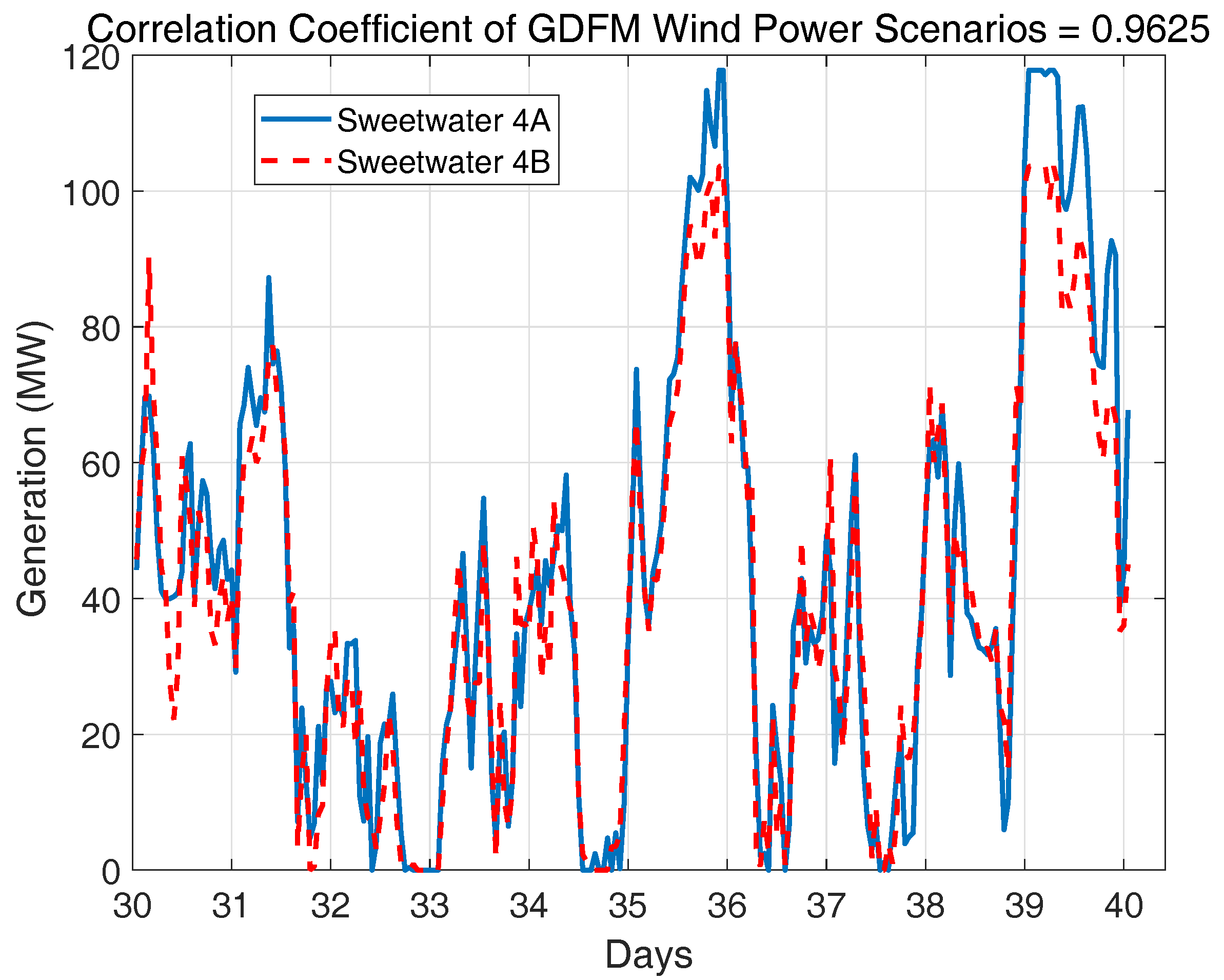
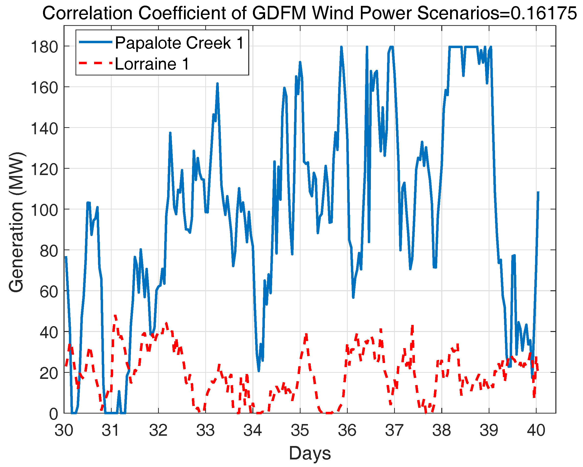
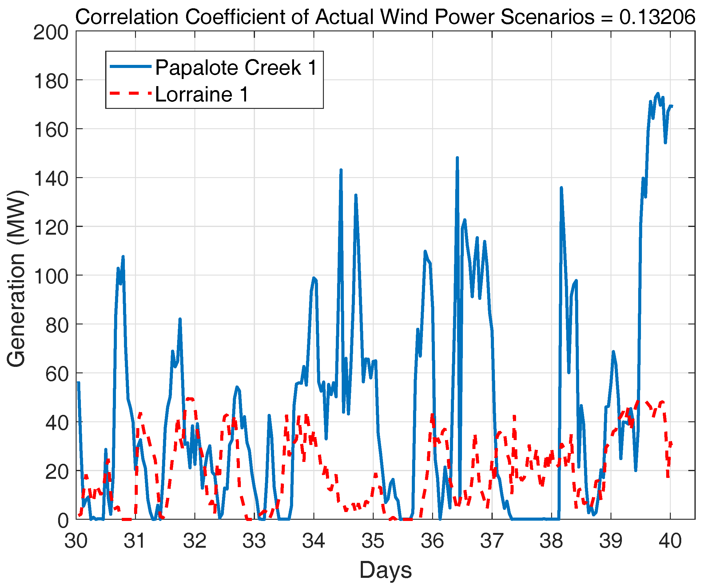
  • The forecasted future scenarios through the GDFM can represent the spatial and temporal correlations among wind power and can fully capture the uncertainty information of the wind power.
  • We modify the ABC algorithm to quickly find the optimal solution of the stochastic dynamic AC OPF problem.
The structure of the paper is as follows. The GDFM is introduced and verified in Section 2. Section 3 first starts with the traditional OPF, and then the formulation of the stochastic dynamic AC OPF is explained. The original ABC is first introduced in Section 4, followed by the modified ABC for the stochastic dynamic AC OPF. Section 5 shows two case studies with numerical results and analyses based on the IEEE 30-bus test system. Finally, Section 6 describes the implications and concludes the paper.

2. Generalized Dynamic Factor Model

The GDFM utilizes the factor analysis (FA) to reduce the data dimension by representing data in terms of the common latent variables, called factors, so that the computational burden of the multivariate time-series analysis can be reduced significantly. Then, the observed variables are modelled as linear combinations of the latent factors. Finally, the observed variables are represented by the product of factor loadings and dynamic factors [15]. The stochastic correlation structure is inherited in the factor loadings [16]. Furthermore, since the dynamic factors are driven by uncorrelated white noise signals, the GDFM can generate arbitrary numbers of forecasting scenarios by varying the dynamic factors.
The advantages of the GDFM are as follows: (1) the FA is used to overcome the “curse of dimensionality”, which happens when we model the high dimensional time series through the vector autoregressive model; (2) the co-movement between time series is used to overcome the curse of dimensionality, so that all scenarios in the GDFM share the spatial and temporal correlation and statistical characteristics that the actual wind power outputs have; and (3) arbitrary numbers of wind power scenarios can be generated from white noise signals.

2.1. Derivation of the GDFM

The factor analysis model, which is known as the static factor model, has been applied widely in forecasting energy, electricity load and economic indices. For wind power forecasting, those latent variables can be wind speed, air density or wind direction. However, the factor analysis model does not consider the temporal correlation when modelling the latent variables (factors) [17]. On the contrary, the dynamic model, which evolved from the static factor model, can consider the spatial and temporal correlations. In this study, the spatial correlation is measured among various wind farms. Here, “dynamic” means there are time lags in the factor loadings.
The first assumption in the GDFM is that the residuals of the observed wind power matrix X N × T can be decomposed into two components: the common component χ N × T and the idiosyncratic component ξ N × T [18]. The residual of wind power can be obtained by subtracting the seasonality from the observed wind power. The variable N is the number of wind farms, and T is the number of observation periods. The common component represents the portion of wind power that is driven by the latent variables, such as air stream or wind flows, so that nearby wind farms will have similar common components. The idiosyncratic component represents the remaining portion of wind power that could be an instant and unpredictable movement or measurement error of each wind power output, so that each wind farm has a different idiosyncratic component.
The column vector X t = x 1 t , x 2 t , , x N t represents the wind power of N wind farms at time t, where t = 1 , , T . Therefore, the column vector X t at time t can be decomposed as:
X t = χ t + ξ t ,
where χ t N is the common component, and ξ t N is the idiosyncratic component at time t. According to this definition, we also assume that χ and ξ are uncorrelated as:
E [ χ j ξ k T ] = 0 ,
where j , k = 1 , , T .
The second assumption is that χ t is assumed to be driven by the process of Q ( Q < N ) latent variables ϕ Q × T , which is called the dynamic factor. The common component is loaded into each wind power output through the factor loading, which is an N × Q matrix polynomial of M lags. Therefore, the χ t N can be decomposed into the multiplication of the dynamic factor and factor loading A ( L ) as:
χ t = A ( L ) ϕ t = A 0 ϕ t + + A M ϕ t M ,
where the L is the delay operator, and A m N × T . Furthermore, A ( L ) is the polynomial matrix, and it is defined as:
A ( L ) = A 0 L 0 + + A M L M ,
where L i is the delay operator. The multiplication between L i and ϕ t means that the ϕ t is delayed by i, i.e., ϕ t i . Since Q < N , the χ t is rank deficient.
The third assumption is that the dynamic factors ϕ t are in a time-series structure; thus, the vector autoregressive (VAR) model can be used to model ϕ t :
ϕ t = C 1 ϕ t 1 + + C R ϕ t R + ε t .
This can be rearranged into:
ε t = C ( L ) = C 0 ϕ t C R ϕ t R ,
where ε t is the column vector of uncorrelated white noise ε t Q × T , C 0 is identity, R is the order of the model, and C ( L ) Q × Q × ( R + 1 ) is a coefficient matrix. Another way to look at Equation (6) is that ϕ t is driven by ε t , however, the ε t has the same spatial correlation as in the actual residual data, while the goal here is to formulate a series of uncorrelated noise to drive ϕ t so that many scenarios can be synthesized. Guided by this idea, we extract the correlation structure from ε with the Cholesky decomposition [11]:
ε t = H δ t ,
where δ t Q × T is called the dynamic shocks. These shocks are a series of spatially and temporally uncorrelated white Gaussian noise with a mean of zero and a variance of one. In addition, the H is the Q × Q matrix that preserves the correlation structure. Finally, by combining Equations (3) and (5)–(7), the dynamic factor is represented as:
χ t = A ( L ) C ( L ) 1 H δ t ,
which leads to the comprehensive form of the GDFM. Then the question of how to estimate A ( L ) and C ( L ) arises naturally, and the procedure is discussed below.

2.2. Estimation of the GDFM

The estimation of the GDFM starts from estimating the Fourier transform of the covariance matrix of X . At each frequency f m , we can split Σ X ( f m ) N × N × F into Σ χ ( f m ) N × N × F , which is the Fourier transform of the covariance matrix of the χ , and Σ ξ ( f m ) N × N × F , which is the Fourier transform of the covariance matrix of ξ . The variable F represents the number of frequencies.
This splitting process can be described through the eigenvalue decomposition as:
Σ X ( f m ) = G χ ( f m ) Ω χ ( f m ) G χ ( f m ) T + G ξ ( f m ) Ω ξ ( f m ) G ξ ( f m ) T ,
where Ω χ ( f m ) Q × Q × F is the diagonal matrix whose diagonals are the top largest Q eigenvalues of Σ X ( f m ) , and G χ ( f m ) N × Q × F is the corresponding eigenvectors associated with Ω χ ( f m ) . The Ω ξ ( f m ) ( N Q ) × ( N Q ) × F is the diagonal matrix whose diagonals are remaining N Q eigenvalues of Σ X ( f m ) , and G ξ ( f m ) N × ( N Q ) × F is the corresponding eigenvectors associated with Ω ξ ( f m ) . Therefore, in (9) the eigenvalues and eigenvectors of Σ X ( f m ) are spliced into the largest Q eigenvalues and their corresponding eigenvectors, and the remaining eigenvalues and their corresponding eigenvectors. Then, by calculating the inverse Fourier transform of each frequency response, χ and ξ in (1) are estimated. This process is called the dynamic principal component analysis (DPCA). Since the only data we can observe is the wind power output data, it is reasonable to assume that dynamic factors can be obtained through filter B ( L ) Q × N × M as:
ϕ t = B ( L ) X t .
In order to forecast wind power scenarios, we estimate the A ( L ) and B ( L ) . Rearranging (1), (3) and (10), ξ t can be written as:
ξ t = X t A ( L ) B ( L ) X t .
The goal is to find the proper values of A ( L ) and B ( L ) to minimize the sum of the variance of ξ t for all t. In other words, we want to minimize the diagonal terms of the covariance matrix of ξ t :
Γ ξ = E X A ( L ) B ( L ) X X A ( L ) B ( L ) X T ,
where Γ ξ is the covariance matrix of ξ , and T is the transpose operator. The next step is to minimize the trace of Γ ξ . The ξ is estimated by splitting the eigenvalues in (9).
Therefore, the solutions for this problem are obtained through the DPCA and Courant-Fisher Theorem [19]. The A ( L ) corresponds to the G χ ( L ) N × Q × F , which are the corresponding eigenvectors associated with the top largest Q eigenvalues of Γ t χ at all lags. Furthermore, the B ( L ) corresponds to ( G χ ( L ) ) T Q × N × F , which are the corresponding eigenvectors associated with the remaining eigenvectors of Γ t ξ . According to (3) and (10), the χ t can be estimated through:
χ t = G χ ( L ) G χ ( L ) T X t .
Again, according to (10), since B ( L ) equals G χ ( L ) T , the ϕ t is estimated through:
ϕ t = G χ ( L ) T X t .
The next step is to synthesize χ t as a function of δ t . In other words, C ( L ) needs to be estimated. For the given VAR process as shown in (5), the coefficients can be estimated through the Yule-Walker Equation [20].
Until now, we define the GDFM and introduce the way to estimate the parameters in the GDFM from the observation data. In the next subsection, we explain the way to forecast the future wind power by using the GDFM.

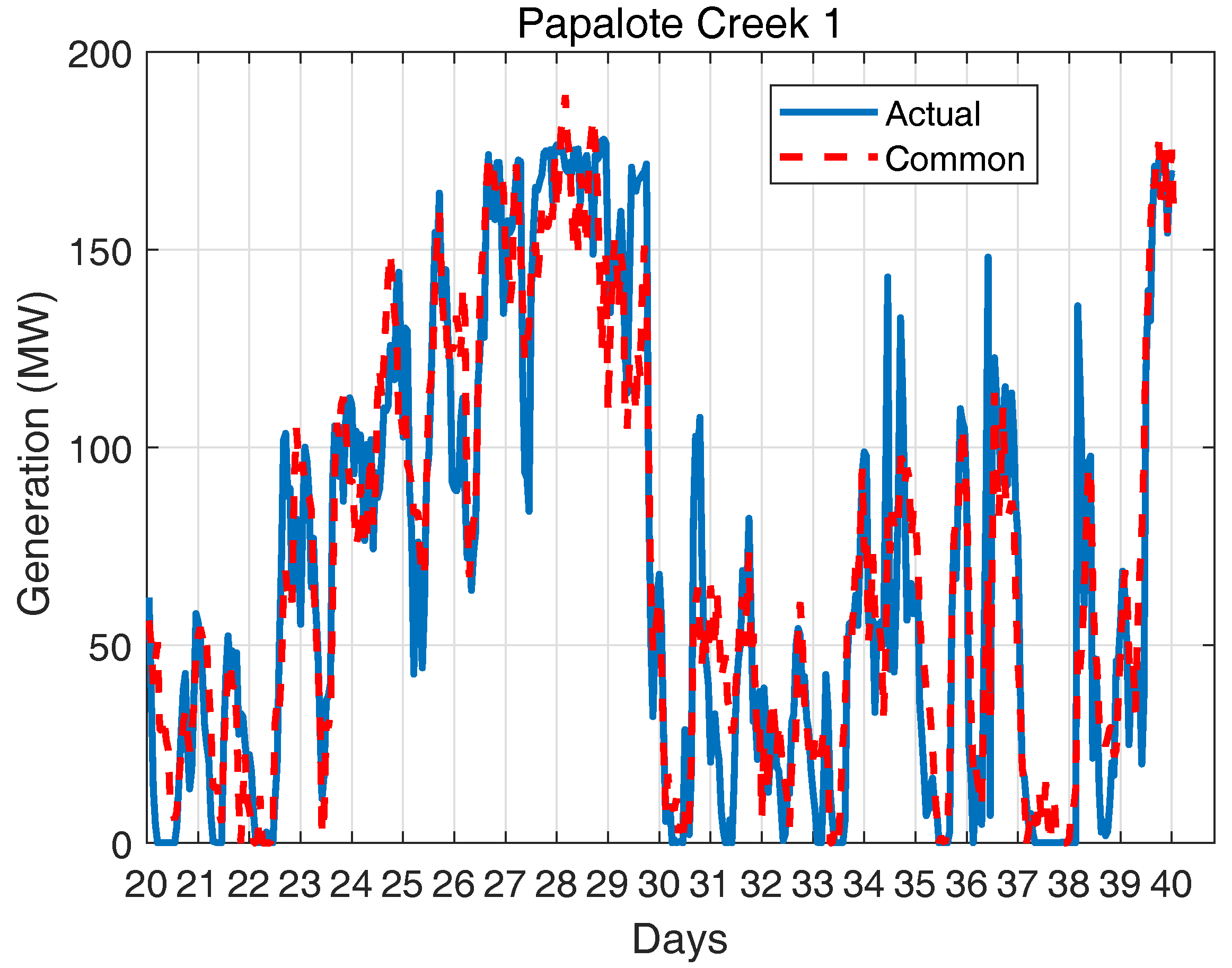
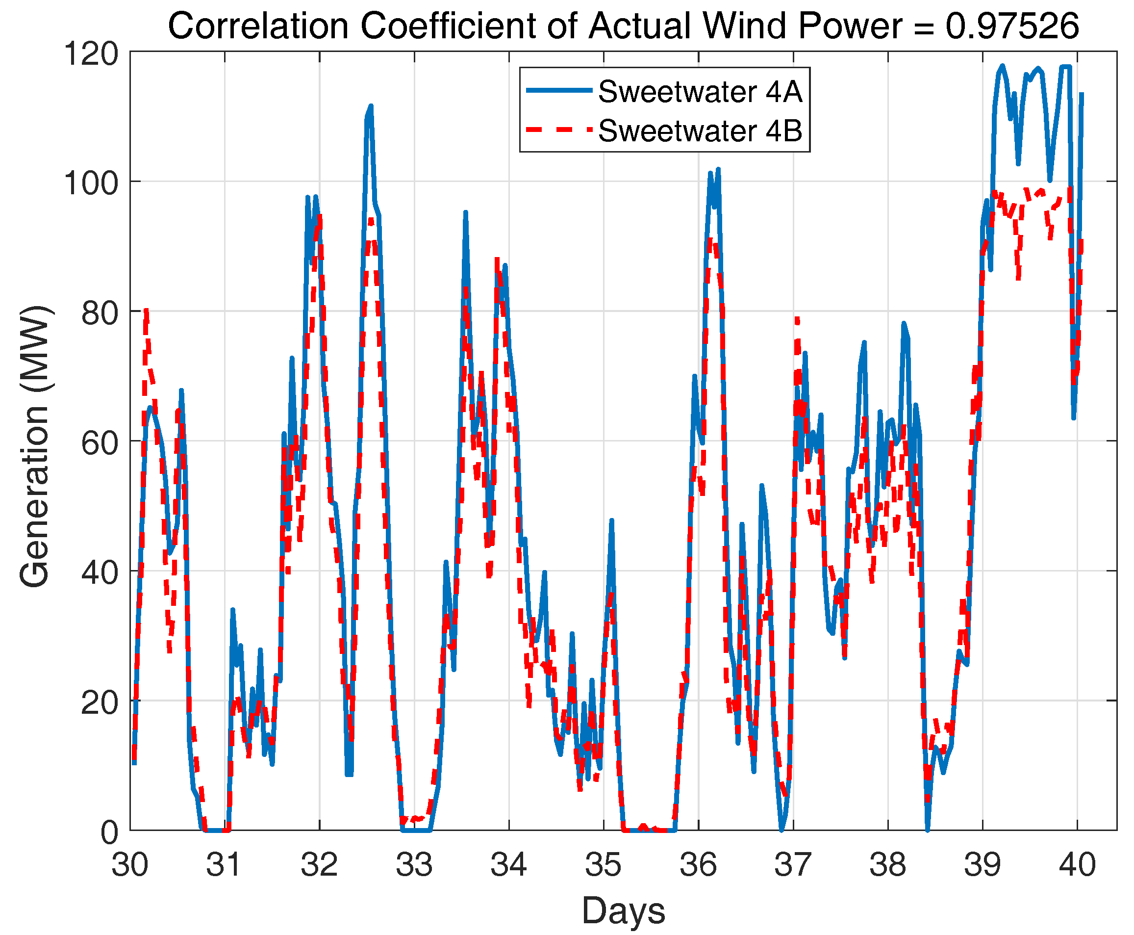
2.3. Forecast Using the GDFM

As mentioned above, our first contribution is to forecast future wind power scenarios of multiple wind farms through the GDFM, which was originally developed to generate current or future wind power scenarios. The key idea is to have zero future error as the best estimate for the dynamic shocks. For the GDFM, the χ t k t can be estimated as:
χ t + k t = A ( L ) C ( L ) 1 H δ t + k t ,
where k is the future steps past the end of the observed series. The superscript t is to be read as “given data up to time t”. Therefore, to forecast over the next 24 h, the columns in the dynamic shocks, δ t + 1 , , δ t + 24 are set to zero. The forecast result is provided in Figure 1. We also compare the performance of the GDFM to the performance of the persistent forecasting model and the performance of the autoregressive (AR) model with order two. In the persistent model, we assume that the last observed value is considered as a forecasted value.
Furthermore, the formulation in (15) shows that multiple future wind power scenarios can be generated simultaneously by using the common characteristics of correlated scenarios so that we can reduce the computational cost and time to forecast future wind power scenarios. This clearly proves our second contribution.
We also compare the performance of the GDFM to performances of other forecasting models, such as the persistent model and AR model. We also test the vector autoregressive (VAR) model, but it cannot forecast the wind power outputs of 90 wind farms because of the short memory. Our machine has 12 GB memories, but it cannot estimate the VAR.
As shown in the Figure 1, there are 30 forecasted future scenarios plotted in blue lines, the forecasts from the AR(2) is plotted in a red dot line, and the forecasts from the persistent model is plotted in a magenta rhombus line. Furthermore, the historical wind power is plotted in a black line, and the actual future wind power is plotted in a black square line. The forecast can capture the trend of actual wind power, and the generated scenarios are used by stochastic programming to make decisions under the high penetration level of intermittent wind power.
The root mean square errors (RMSE)s of forecasting models with respect to the forecasting horizons are plotted in Figure 2, and the mean absolute errors (MAE)s of the forecasting models with respect to the forecasting horizons are plotted in Figure 3. In Figure 2 and Figure 3, the forecasts of the persistent model are plotted in a blue line, the forecasts of the AR(2) are plotted in a red circle line, and the forecasts of the GDFM are plotted in a black square line. When the performance of the GDFM is measured, the dynamic shock is assumed to be zero so that we can have a single scenario.
In Figure 2 and Figure 3, we can observe that the performance of the GDFM is higher than those of other forecasting models. Furthermore, when the performance is measured by the RMSE, the performance difference between the GDFM and other forecasting models is significant. It means that the GDFM can forecast wind power outputs that are not extremely far from actual wind power outputs. For some forecasting horizons, the performance of the GDFM is lower than other forecasting models, but for most of forecasting horizons, the GDFM performs better than other forecasting models. Besides, it should be emphasized that the GDFM can keep the stochastic correlation structure among wind power outputs, but other forecasting models cannot.
We also calculate the average RMSE and MAE in Table 1. It is clearly shown that the GDFM has the best performance among three forecasting models.
In this subsection, we forecast the future wind power scenarios by having zero dynamic shocks. In the next subsection, we verify whether the forecasted scenarios are spatially and temporally correlated. It should be noted that the forecasting accuracy of the GDFM scenarios will be tested in the Section 5.

2.4. Verification of the Spatially and Temporally Correlated Scenarios

Our third contribution is that the scenarios forecasted by the GDFM are spatially and temporally correlated. The procedures of synthesizing scenarios can be summarized as follows: (a) χ ^ , ξ ^ , and ϕ ^ are estimated from data set X (the “hat” denotes for the estimated value); (b) since dynamic factors ϕ can be modelled as a VAR process, the noise term in VAR model can be estimated as ε ^ ; (c) scenarios of χ ^ are synthesized by giving δ , which are uncorrelated noises into the model as denoted by (7); and (d) the X ^ is finally synthesized by adding χ ^ with ξ ^ , and the estimation of the original data can be obtained by adding seasonality and reversing the normalization process. Figure 4 gives the wind farms in Texas, which are marked in red. The N = 23 wind farm observation data from the Electric Reliability Council of Texas (ERCOT) is used. They are grouped in three regions, Mountain King (left), Sweetwater (top), and Corpus Christi (right), as circled in Figure 4. The hourly data is from 1 January to 31 March in 2013 for a total of T = 24 × 90 = 2160 h. The forecasting period is 24 h ahead in the historical data, which is 1 April 2013.
The original data is preprocessed as follows: (1) for each wind farm, the average wind power output across the total of measured period is subtracted from the raw wind power output; (2) the residuals are divided by the standard deviation of the wind power output of each single wind farm; and (3) the diurnal pattern of the wind power output of each single wind farm is extracted. The Steps 1 and 2 are the standardizing process and the Step 3 is the process of removing seasonality. The periodic component at each hour is estimated by averaging wind power outputs measured at the same hour. The process to generate the periodic component is as follows. First, the wind power outputs X 23 × 24 × 90 are reshaped by 24 h and 90 days as Y 23 × 24 × 90 . Then the mean of each hour over 90 days is stacked as Z 23 × 24 , and the daily pattern is estimated by averaging the reshaped wind power at every hour. Finally, the daily pattern is subtracted from the X . It should be noted that after synthesizing preliminary normalized scenarios using residuals, the reverse process of preprocesses is applied to the preliminary normalized scenarios to the obtain final scenarios.
The model is also verified in Figure 5 with the power spectral density (PSD) plot of the scenario in the frequency domain. The PSD indicates the contributions of different frequency components. Note that the x-axis is changed to “period”, the reciprocal of “frequency” for easier interpretation. It is found that the frequency response of the wind power data from the Papalote Creek 1 has a very strong component corresponding to “24-h period”. Similarly, the synthesized PSD corresponds with the actual wind data.
Figure 6 shows the comparison between actual wind power and its common component at the Papalote Creek 1 (Corpus Christi region). It is observed that the common component in a red line can catch the trend of the actual wind power, i.e., it is similar with the actual measurements in terms of ramp, maximum, minimum, and overall shape.
As described earlier, one of the advantages is that the GDFM can capture the co-movement of synthesized scenarios, i.e., the synthesized scenarios of different wind farms have similar correlations as the actual wind power outputs do. Figure 7 and Figure 8 have demonstrated this with the correlation coefficients of 0.97526 and 0.96059, respectively, for the actual wind power and the synthesized scenarios of SweetWater 4A and SweetWater 4B wind farms, which are two very close wind farms.
Similarly, Figure 9 and Figure 10 show the correlations between Papalote Creek 1 (Corpus Christi region) and Lorraine 1 (SweetWater region) for both actual and generated scenarios. The farther the wind farms are located, the less correlated the wind power outputs are. Therefore, since the distance between the Papalote Creek 1 and Lorraine 1 is around 400 miles, the correlation coefficient between these two wind farms is low.
In this subsection, we see that the GDFM scenarios are spatially and temporally correlated. In the next section, we formulate the stochastic and dynamic AC OPF problem where the GDFM scenarios will be used.

3. Stochastic Dynamic Optimal Power Flow

In this section, the stochastic and dynamic AC OPF problem is formulated. The objective of the AC OPF problem is to minimize fuel costs by determining the optimal reactive and active power outputs, while satisfying voltage and apparent power constraints. Furthermore, the dynamic OPF problem solves this AC OPF over a period of time. Moreover, the stochastic OPF problem solves the AC OPF while considering the uncertainty stemming from the stochastic wind power output. In the stochastic OPF problem, the uncertainties are captured by scenarios, and thus the mathematical formulation is:
minimize x f ( x , u )
subject to g ( x , u ) = 0
h ( x , u ) 0 ,
where vector u represents the decision/control/independent variables over 24 h, which include the generator real power P G (except the power at the slack bus), the generator bus voltage V G , the transformer tap T, and the shunt compensator Q C at selected buses. The vector x is state/dependent variables, which include the real power P G 1 at a slack bus, voltages V L at a load bus, reactive power Q G at a generator bus, and loadings S L of transmission lines.
The objective function is the sum of total fuel costs and real power losses. The fuel cost is:
F 1 = t = 1 24 i = 1 N G a i P G i t 2 + b i P G i t + c i ,
where a i , b i , c i , and P G i t denote the quadratic fuel cost coefficients and real power at the i-th unit at time t, and N G is the number of generators. The real power loss is due to the power flowing through transmission lines. The objective function for power loss can be mathematically formulated as follows:
F 2 = t = 1 24 i = 1 N l r k r k 2 + x k 2 V i t 2 + V j t 2 2 V i t V j t cos δ i t δ j t ,
where N l is the total number of transmission lines, r k is the resistance of the transmission line k, and x k is the reactance of transmission line k. Furthermore, V i t , V j t , δ i t , and δ j t are the voltages and angles at bus i and j between the transmission line k at time t, respectively. In this paper, F 1 , and F 2 are the two cost functions considered for case studies. The equality constraints g from (17) are the AC power flow balance equations at each bus representing that the power flowing into that specific bus is equal to the power flowing out, which are defined as:
P i t = V i t j = 1 N V j t Y i j cos ( δ i t δ j t θ i j ) Q i t = V i t j = 1 N V j t Y i j sin ( δ i t δ j t θ i j ) ,
where N is the total number of buses, P i t and Q i t are the injected real and reactive power at bus i at time t, and Y i j and θ i j are the elements in Y admittance matrix. Inequality constraints h in (18) include generator limits, ramp rate constraints of generators, tap position of transformers, shunt capacitor constraints, security constraints, load bus voltage, and transmission line flows [4]. The advantage of the stochastic optimization is that the optimal solution that can minimize the expected cost of all scenarios can be obtained. Therefore, the stochastic dynamic AC OPF is formulated to minimize the expected value E F of the objective function over all scenarios as:
E V = s = 1 S p r o b s t = 1 24 F t ,
where F t is cost function from (19) to (20) at time t, p r o b s is the probability of scenario s which quantifies the likelihood of that scenario, and S is the total number of scenarios. Since we assume that every scenario is independent from others, the probability for each scenario is 1 / S . Thus, the stochastic dynamic AC OPF can be summarized to minimize (22) while complying with the equality and inequality constraints.
In this section, we build the stochastic and dynamic AC OPF formulation, but it is impossible to solve this formulation numerically. Therefore, in the next section, we introduce the artificial bee colony method to solve the AC OPF and modify the method to solve the problem more quickly.

4. Solution Methodology

It is difficult to solve a mixed integer nonlinear problem (MINLP) accurately without a simplification. However, if we use various heuristic optimization techniques, we can find an approximate but reliable solution without simplification. Thus, in this work, we adopt the artificial bee colony (ABC) and modify it to tackle the stochastic and dynamic AC OPF.

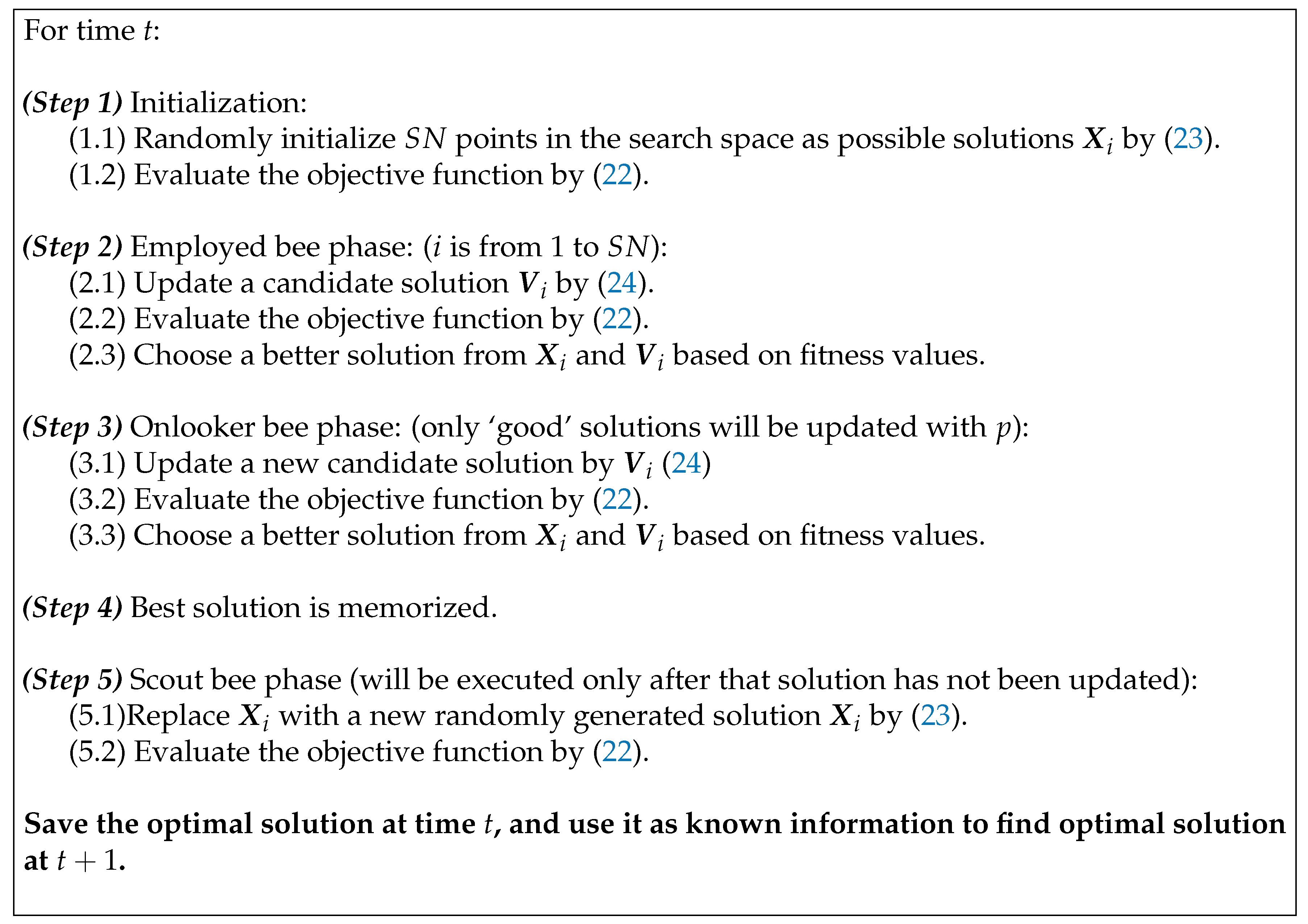
4.1. Original ABC Algorithm

Our last contribution in this manuscript is to modify the ABC algorithm in order to reduce the computational time to find the optimal solution of the stochastic dynamic AC OPF problem. The original inspiration of the ABC is from the foraging behaviours of natural honey bee swarms—through communication and cooperation, honey bees carry out a common objective. In the original ABC algorithm in [21], the initial artificial bees are spread out randomly in a multidimensional search space. Each artificial bee can store current information and communicate with other bees. The ABC has been used in various applications [22,23]. There are three types of bees: employed bees, onlooker bees, and scout bees. Employed bees search for food sources, record the good food sources, and share the information with onlooker bees. The onlooker bees search for better food sources near known good sources, and scout bees randomly search at farther distances to find more abundant food sources. First, each vector solution X i = X i , 1 , X i , 2 , , X i , D is initialized randomly within the limits of the control variables as follows:
X i , j = X i , j min + r a n d ( 0 , 1 ) × ( X i , j max X i , j min ) ,
where X i , j min and X i , j max are the lower and upper bounds for the vector in the dimension i and j. The i is from 1 to S N , and j can be randomly chosen from 1 to D. Furthermore, the SN is the number of both employed and onlooker bees, and the D is the number of optimization parameters.
Furthermore, r a n d ( 0 , 1 ) generates uniformly distributed random numbers between ( 0 , 1 ) . The onlooker bee finds the nectar continuously. In the employed bee phase, each bee searches for rich artificial food sources by updating the current food source (solutions) based on the information collected in their neighbourhood and assesses the nectar of the new food source (solutions). The current solution is updated by the search equation, which is defined as:
V i , j = X i , j + Φ i , j × ( X i , j X k , j ) ,
where k is an integer different from i, randomly chosen from the range [ 1 , S N ] , and ϕ i , j is a random number from [ 1 , 1 ] . If the updated solution has better nectar than the old one, the employed bee will memorize the new solution and discard the old one. Otherwise, they will keep the old solutions. This process is called “greedy selection”. Then, onlooker bees will continue updating those solutions with high nectar using the roulette wheel selection scheme, which is similar to the genetic algorithm (GA). Finally, the scout bee will execute only if any bee is trapped in a local minimum. The equation in (23) is used by a scout bee to randomly start a new search once there is a bee in a local minimum.
In this subsection, we introduce the original ABC method to solve the AC OPF. However, in order to reduce the computational time, we suggest the modified ABC method in the next subsection.

4.2. Modified ABC for the Stochastic Dynamic AC OPF
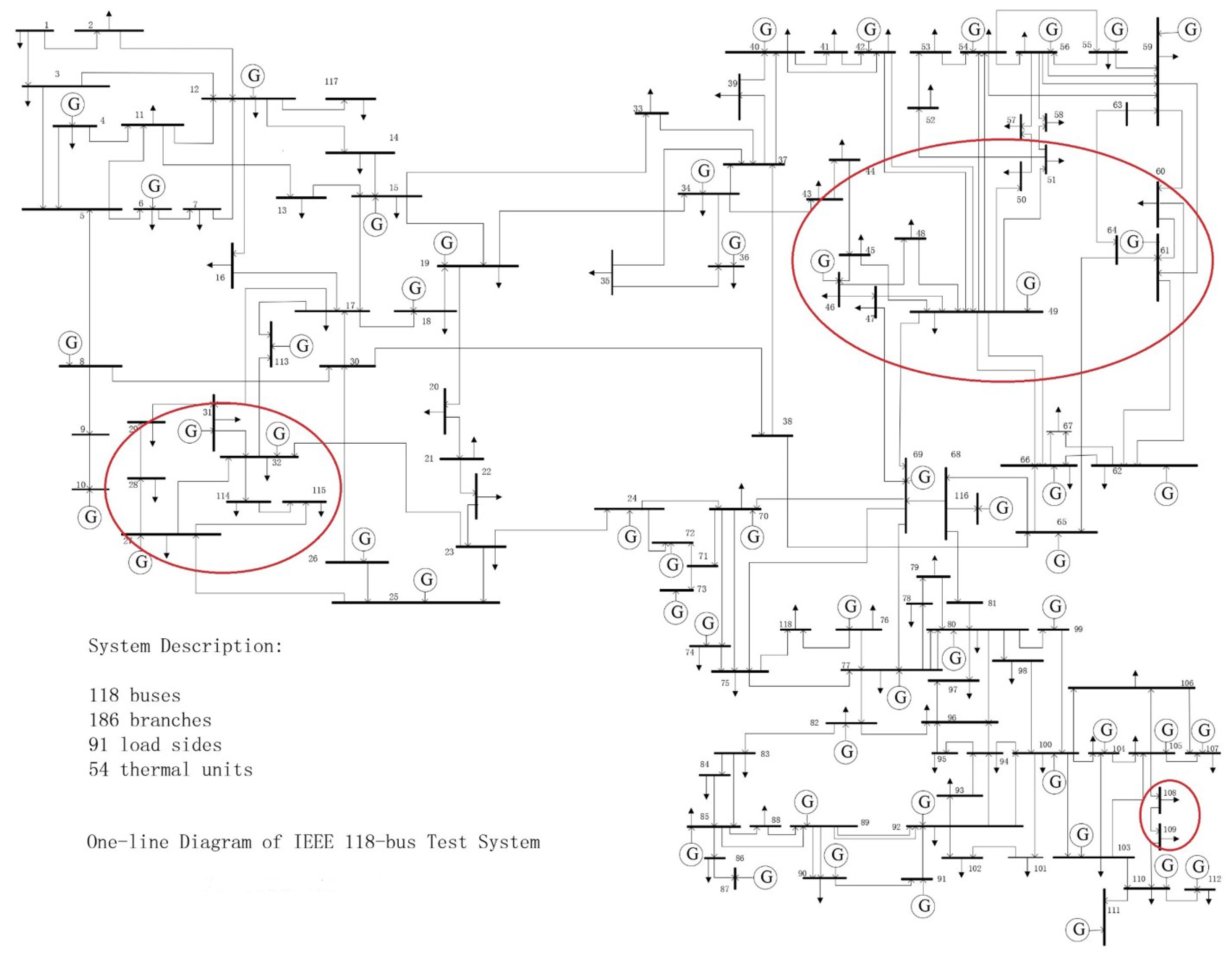
The original ABC can be computationally costly in solving a problem involving many control variables. Therefore, we have modified the ABC, called the modified ABC (MABC), to tackle the dynamic optimization problem recursively in order to reduce the computational time. The procedure of the MABC is shown in the Figure 11. The optimization at each hour is based on the information in previous hours. During the optimization process, the ramp constraints are also considered. Furthermore, in this process, the MABC can have fewer power flow decision variables than the ABC with the static optimization. If the original ABC is used, the decision vector, which consists of all generator power and voltage magnitudes, transformer taps, and shunt capacitors over 24 h, is significantly large.
In this section, we introduce the original ABC method and its modified ABC method to solve the AC OPF in reduced computational time. In the next section, we will solve the AC OPF problem by using the modified ABC method. In this process, the test power system is operated based on the forecasted GDFM scenarios.

5. Case Studies

We conduct several case studies to evaluate the effectiveness of the proposed method. The modified ABC and the stochastic processes are implemented in the modified IEEE 118-bus test system. In the modified system, there are 23 wind farms located at three regions, which are circled in red in Figure 12, based on the approximated wind farm geographic locations. The computer used for simulation has 3.4 GHz Intel core i7 Processor (R2015a, MathWorks, Natick, MA, USA) and 32 GB RAM. The AC power flow is calculated by the MATPOWER package (6.0, PSERC, Ithaca, NY, USA) [24].

5.1. Case 1: Quadratic Fuel Cost Minimization

Case 1 is a standard OPF problem with the cost function in quadratic form. We can find the data for the IEEE 118-bus test system with control variable limits and fuel cost coefficients in [25]. There are a total of 130 control variables, which consist of 53 real power outputs at PV buses, voltage magnitudes of all 54 generator buses, nine transformer taps, and 14 shunt capacitors. The objective in this case is to minimize the total generator fuel cost in (19). Transformer taps and shunt capacitors are discrete variables, which increases the complexity to the problem.
Table 2 summarizes the comparison results. The load profile was for 21 December 2014 obtained from ERCOT [26] and is scaled to fit the size of this problem. Note that 15 scenarios are generated by the GDFM for each farm, and that they are correlated with each other. However, if random scenarios are used to represent the uncertainty, it would have been 15 23 scenarios without certain scenario reduction techniques, which is not feasible to solve. In this study, we chose 100 uncorrelated random scenarios. Because of the fact that GDFM can provide correlated scenarios, only a limited number of scenarios needed to be generated so that the computational cost for stochastic optimization is significantly reduced compared with random scenarios. Table 2 also compares the performance of the ABC with the MABC in computational time (s) and total fuel cost ($), where it is found that by using the MABC, the computational cost and generation cost can be reduced compared to using the ABC.

5.2. Case 2: Loss Minimization

In this case, the objective is to minimize the total real power loss defined in (22). The control and state variables are identical to the previous case. From the Table 3, a similar conclusion is drawn that the MABC is able to reduce computational cost and power loss more than the ABC. Only the correlated scenarios can represent a meaningful and real uncertainty from wind power forecasting.
In this section, we could see that the MABC method outperforms the ABC method for the quadratic fuel cost minimization and transmission loss minimization cases. Furthermore, the OPF based on the GDFM scenarios has a lower generation cost than the randomly generated scenarios since the forecasted GDFM scenarios can represent the spatially and temporally correlated actual wind power.

6. Conclusions

This paper shows that the complex stochastic dynamic AC OPF under high wind power penetration can be solved based on the wind power forecasting scenarios of the GDFM. The GDFM is verified in both time and frequency domains. Since the GDFM scenarios are spatially and temporally correlated, the benefits of using scenarios by GDFM are as follows: (1) only a limited number of scenarios need to be generated to represent the uncertainty so that the computational cost for stochastic optimization can be greatly reduced; and (2) correlated scenarios can represent a more realistic forecasting where all wind farms in a close area are spatially correlated under the same weather pattern.
The MABC is used to solve the stochastic dynamic AC OPF, which is non-differentiable, non-convex, and mixed integer optimization problem. Besides, the MABC does not transform the AC OPF problem as conventional optimization techniques. The MABC is tested on the IEEE 118-bus system integrated with 23 wind farms. It is shown that the MABC with the GDFM scenarios can not only handle the fuel cost minimization, but also the complex objective function for the power loss of transmission lines while reducing the computation time.

Acknowledgments

This work was supported by the Korea Institute of Energy Technology Evaluation and Planning (KETEP) and the Ministry of Trade, Industry & Energy (MOTIE) of the Republic of Korea (No. 20174030201660) and Basic Science Research Program through the National Research Foundation of Korea (NRF) funded by the Ministry of Education (No. 2017035806).

Author Contributions

Wenlei Bai prepared the first draft of this manuscript, implemented the ABC optimization algorithm, and solved the AC OPF. Duehee Lee developed the GDFM model and GDFM forecasting model, contributed to the preparation of the data bases, and revised the manuscript. Kwang Y. Lee organized the research team, proofread the manuscript, and provided research formulation and direction.

Conflicts of Interest

The authors declare no conflict of interest.

References

  1. Calif, R.; Schmitt, F.G. Multiscaling and joint multiscaling of the atmospheric wind speed and the aggregate power output from a wind farm. Nonlinear Process. Geophys. 2014, 21, 379–392. [Google Scholar] [CrossRef] [Green Version]
  2. Calif, R.; Schmitt, F.G.; Huang, Y. Multifractal description of wind power fluctuations using arbitrary order Hilbert spectral analysis. Phys. A Stat. Mech. Appl. 2013, 392, 4106–4120. [Google Scholar] [CrossRef]
  3. Wu, G.; Sun, L.; Lee, K.Y. Disturbance rejection control of a fuel cell power plant in a grid-connected system. Control Eng. Pract. 2017, 60, 183–192. [Google Scholar] [CrossRef]
  4. Bai, W.; Eke, I.; Lee, K.Y. Heuristic optimization for wind energy integrated optimal power flow. In Proceedings of the 2015 IEEE Power Energy Society General Meeting, Denver, CO, USA, 26–30 July 2015; pp. 1–5. [Google Scholar]
  5. Bai, W.; Eke, I.; Lee, K.Y. Improved artificial bee colony based on orthogonal learning for optimal power flow. In Proceedings of the 2015 18th International Conference on Intelligent System Application to Power Systems (ISAP), Porto, Portugal, 11–16 September 2015; pp. 1–6. [Google Scholar]
  6. Botterud, A.; Zhou, Z.; Wang, J. Use of Wind Power Forecasting in Operational Decisions; Technical Report ANL/DIS-11-8; Argonne National Laboratory: Chicago, IL, USA, 2011.
  7. Zhu, X.; Genton, M.G. Short-Term Wind Speed Forecasting for Power System Operations. Int. Stat. Rev. 2012, 80, 2–23. [Google Scholar] [CrossRef]
  8. Monteiro, C.; Bessa, R.; Miranda, V.; Botterud, A.; Wang, J. Wind Power Forecasting: State-of-the-Art; Technical Report ANL/DIS-10-1; Argonne National Laboratory: Chicago, IL, USA, 2009.
  9. Huang, Z.; Chalabi, Z. Use of time-series analysis to model and forecast wind speed. J. Wind Eng. Ind. Aerodyn. 1995, 56, 311–322. [Google Scholar] [CrossRef]
  10. Xie, L.; Gu, Y.; Zhu, X.; Genton, M.G. Short-Term Spatio-Temporal Wind Power Forecast in Robust Look-ahead Power System Dispatch. IEEE Trans. Smart Grid 2014, 5, 511–520. [Google Scholar] [CrossRef]
  11. Morales, J.; Mínguez, R.; Conejo, A. A methodology to generate statistically dependent wind speed scenarios. Appl. Energy 2010, 87, 843–855. [Google Scholar] [CrossRef]
  12. Lee, D.; Baldick, R. Load and Wind Power Scenario Generation Through the Generalized Dynamic Factor Model. IEEE Trans. Power Syst. 2017, 32, 400–410. [Google Scholar] [CrossRef]
  13. Wang, J.; Shahidehpour, M.; Li, Z. Security-Constrained Unit Commitment With Volatile Wind Power Generation. IEEE Trans. Power Syst. 2008, 23, 1319–1327. [Google Scholar] [CrossRef]
  14. Lee, K.Y.; El-Sharkawi, A.M. Mordern Heuristic Optimization Techniques: Theory and Applications to Power Systems; John Wiley & Sons: Hoboken, NJ, USA, 2008. [Google Scholar]
  15. Lee, D.; Lee, J.; Baldick, R. Wind power scenario generation for stochastic wind power generation and transmission expansion planning. In Proceedings of the 2014 IEEE PES General Meeting | Conference Exposition, National Harbor, MD, USA, 27–31 July 2014; pp. 1–5. [Google Scholar]
  16. Forni, M.; Gambetti, L. The dynamic effects of monetary policy: A structural factor model approach. J. Monetary Econ. 2010, 57, 203–216. [Google Scholar] [CrossRef]
  17. Van Nieuwenhuyze, C. A Generalised Dynamic Factor Model for the Belgian Economy—Useful Business Cycle Indicators and GDP Growth Forecasts; Technical Report 80; National Bank of Belgium Working Paper; National Bank of Belgium: Brussels, Belgium, 2006. [Google Scholar]
  18. Forni, M.; Hallin, M.; Lippi, M.; Reichlin, L. The Generalized Dynamic Factor Model. J. Am. Stat. Assoc. 2005, 100, 830–840. [Google Scholar] [CrossRef]
  19. Brillinger, D.R. Time Series: Data Analysis and Theory; SIAM: Philadelphia, PA, USA, 1981. [Google Scholar]
  20. Reinsel, G.C. Elements of Multivariate Time Series Analysis; Spinger and Business Media: Berlin/Heidelberg, Germany, 2012. [Google Scholar]
  21. Karaboga, D. An Idea Based on Honey Bee Swarm for Numerical optimization; Erciyes University: Kayseri, Turkey, 2005. [Google Scholar]
  22. Bai, W.; Lee, K.Y. Modified optimal power flow on storage devices and wind power integrated system. In Proceedings of the 2016 IEEE Power and Energy Society General Meeting (PESGM), Boston, MA, USA, 17–21 July 2016; pp. 1–5. [Google Scholar]
  23. Bai, W.; Abedi, M.R.; Lee, K.Y. Distributed generation system control strategies with PV and fuel cell in microgrid operation. Control Eng. Pract. 2016, 53, 184–193. [Google Scholar] [CrossRef]
  24. Zimmerman, R.D.; Murillo-Sanchez, C.E.; Thomas, R.J. MATPOWER: Steady-State Operations, Planning, and Analysis Tools for Power Systems Research and Education. IEEE Trans. Power Syst. 2011, 26, 12–19. [Google Scholar] [CrossRef]
  25. Lee, K.Y.; Park, Y.M.; Ortiz, J.L. A United Approach to Optimal Real and Reactive Power Dispatch. IEEE Trans. Power Appar. Syst. 1985, PAS-104, 1147–1153. [Google Scholar] [CrossRef]
  26. Electric Reliability Council of Texas. Technical Report. Available online: http://www.ercot.com/gridinfo/load/load_hist/ (accessed on 21 November 2017).
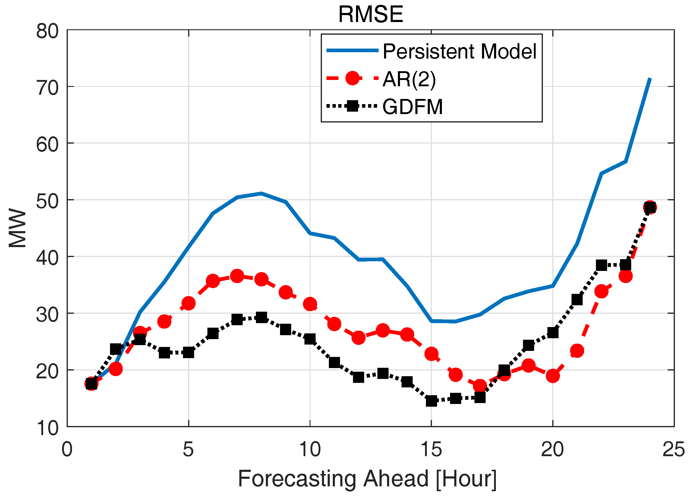
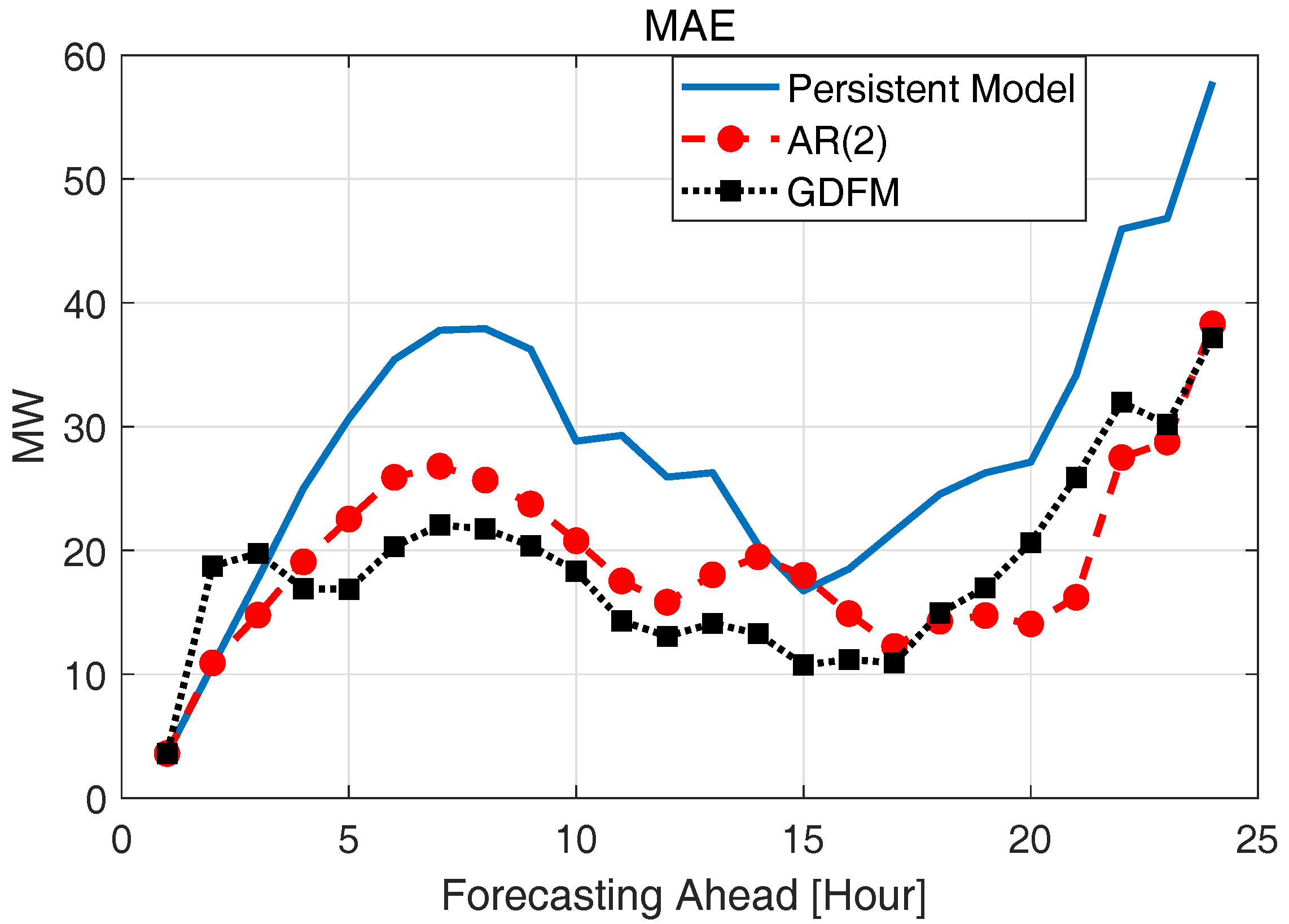
Figure 1. Wind power forecasts at #29 wind farm.
Energies 10 02138 g001
Figure 2. The RMSE performance of forecasting models.
Energies 10 02138 g002
Figure 3. The MAE performance of Forecasting models.
Energies 10 02138 g003
Figure 4. Wind farms in Texas.
Energies 10 02138 g004
Figure 5. The PSD of actual wind power and synthesized wind power at Papalote Creek 1.
Energies 10 02138 g005
Figure 6. Actual wind power and its common component at Papalote Creek 1 (corpus Christi region).
Energies 10 02138 g006
Figure 7. Actual wind power scenarios from the Sweetwater 4A and Sweetwater 4B.
Energies 10 02138 g007
Figure 8. Forecasted wind power scenarios from the Sweetwater 4A and Sweetwater 4B.
Energies 10 02138 g008
Figure 9. Actual wind power scenarios from uncorrelated wind farms, Papalote Creek 1 and Lorraine 1.
Energies 10 02138 g009
Figure 10. Forecasted wind power scenarios from uncorrelated wind farms, Papalote Creek 1 and Lorraine 1.
Energies 10 02138 g010
Figure 11. The overall structure of the modified ABC for dynamic optimization.
Energies 10 02138 g011
Figure 12. Modified IEEE 118 bus system.
Energies 10 02138 g012
Table 1. Average Performance of Forecasting Models.
MethodsPersistent ModelAR(2)GDFM
RMSE [MW]39.973427.746125.0448
MAE [MW]28.554619.3218.05
Table 2. Comparison of computing time and optimal costs in Case 1.
Methods RandomGDFMRandomGDFM
(Minute)(Minute)($)($)
ABC305.656.73,284,8563,264,344
MABC120.330.33,254,2213,120,322
Table 3. Comparison of computing time and minimum loss in Case 2.
Methods RandomGDFMRandomGDFM
(Minute)(Minute)(MW)(MW)
ABC250.480.51201.41193.8
MABC110.342.51178.51128.4

