Article

A Two-Level Optimal Scheduling Strategy for Central Air-Conditioners Based on Metal Model with Comprehensive State-Queueing Control Models

1
Electric Power Planning & Engineering Institute, Beijing 100120, China
2
Key Laboratory of Smart Grid of Ministry of Education, Tianjin University, Tianjin 300072, China
3
State Grid Energy Research Institute, Changping District, Beijing 102249, China
*
Author to whom correspondence should be addressed.
Energies 2017, 10(12), 2133; https://doi.org/10.3390/en10122133
Submission received: 27 October 2017 / Revised: 10 December 2017 / Accepted: 11 December 2017 / Published: 14 December 2017

Abstract

:
Unlike some thermostatically controlled appliances (TCAs) with small capacities, Central Air-conditioner (CAC) has huge potential for demand response because of its large capacity. This paper presents a new CAC control strategy under multiple constraints. The CAC is modeled by three main modules: CAC central unit, water pumps, and temperature simulation of terminal users. The CAC’s power consumption is mainly determined by users’ load ratio. As the information and communication system have become the central nervous system of the smart grid, big data analysis is of great significance. Assuming that reliable two-way communication systems are preset, an integrated parameter priority list (IPPL) control strategy is used to control and monitor CAC. A new intelligent algorithm, Space Exploration and Unimodal Region Elimination (SEUMRE) algorithm, is introduced for solving the optimization problem of demand response targets generation under multiple constraints with the help of big data analysis. In this paper, influences and constrain factors, such as price and users’ comfortable levels are taken into account to satisfy the need of actual situation. Simulation results show that the proposed approach, when comparing with other typical optimization algorithms, yields better performances and efficiency.

1. Introduction

In recent years, microgrids that are supplied by renewable generation resources, such as photovoltaic or wind power, have received extensive attention worldwide. The State Grid Corporation of China has been building several microgrid demonstration projects that are located in Zhejiang, Guangzhou, and western China. A demonstration microgrid system for a residential community was built in Dongfushan Island, Zhejiang. The microgrid was supplied by a 210-kW wind generation, a 100-kW solar generation with a 200-kW diesel generator, and a 2 V/1200 Ah lead-acid battery storage system. In such a microgrid, an important issue in system operation is to deal with the intermittency of renewable generation resources. Diesel generators (or sometimes gas turbines) and Energy Storage Systems (ESSs) can only provide very limited load balancing services at very high cost.
Recently, demand response (DR) was used as a potential solution to coordinate with ESSs to stabilize renewable power fluctuations. DR had been used to provide energy market and ancillary service functions, such as peak management [1], load shifting [2], primary frequency response [3,4], spinning reserve [5,6,7,8], and voltage stability enhancement [9], traditionally.
Load balance services provided by thermostatically controlled appliances (TCAs), which include residential heating, ventilation, and air-conditioner (HVAC) systems, electric water heaters, and refrigerators, are gaining wider attention. A temperature-priority-list method was used to dispatch the HVAC loads optimally to maintain customer-desired indoor temperature and load diversity [10]. As a follow-up work, a temperature-priority-list algorithm was proposed in [11] using simplified first-order equivalent thermal parameter (ETP) models for TCAs. Thermostat control for TCAs is a typical method to achieve demand response, such as that described by the Fokker-Planck diffusion model proposed in [12], and followed works in [13,14] when considering user comfort-constraints, and active power regulation in wind transmission system [15]. A state-queueing model [16] was proposed to study the state shift behavior of HVAC systems after a change in electricity price, in response to which their thermostat setpoints are changed. Physically-based methodologies for synthesizing the hourly residential HVAC load was developed by Chan et al. [17]. Open communication protocols, internet technologies, HVAC sensors, actuators, control systems, as well as embedded computer hardware and software technologies have made Internet-based HVAC system monitor and control possible [18,19]. A novel real-time optimization approach [20] for two-way direct load control of central air-conditioner chillers was proposed. The proposed optimization approach will minimize the difference between the load required to shed and the load actually shed at each sampling interval. Callaway’s research put more efforts into the population characteristics, where the Markov transition matrix was used to evaluate the power consumptions [21].
In the past research, few papers focused on the demand response strategies of CAC with multi-constraints. A fuzzy-PID (Proportion Integration Differentiation) based method was proposed in [22] to achieve good control effect when considering the air flux, fan speed, and indoor temperature. In [23], the author introduced a refrigerator and a welding machine applied “Neuro-Fuzzy” control, which combined heuristic optimization methods and HVAC control structure. The main contributions of this paper are summarized as follows:
(1)
putting up a new CAC operating status evaluating method aiming to solve the problem of multi-dimensions constraints including pricing, temperature, historical switching number, and users’ willingness;
(2)
based on the CAC operating models and evaluating method, setting up a CAC group joint optimized operation structure with multi-dimensions constraints; and,
(3)
using the new response surface method optimization algorithm, Space Exploration and Unimodal Region Elimination (SEUMRE) is used as the solver of optimization model to calculate the appropriate demand response targets that the CAC groups need to undertake.
The remainder of this paper is organized as follows. A detailed introduction of structure and models, which include CAC modules, electricity price, switching number, is given in Section 2. The SEUMRE algorithm and IPPL strategy are discussed in Section 3. Simulation results are then presented in Section 4, followed by conclusions and recommendations for future work in Section 5.

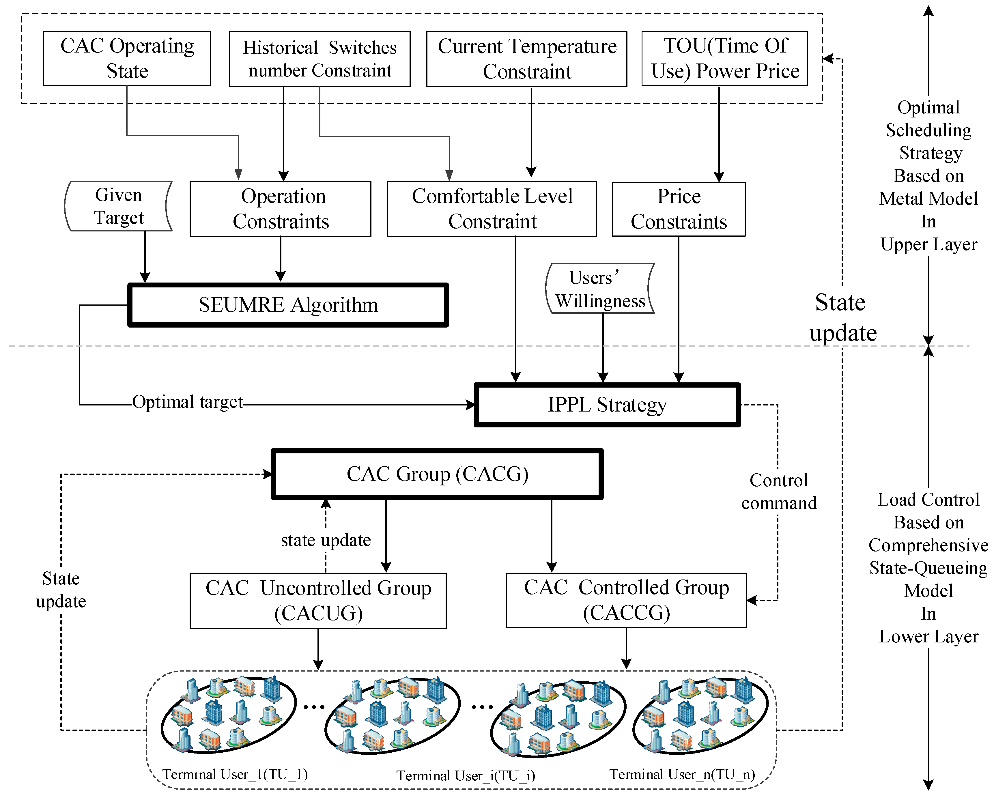
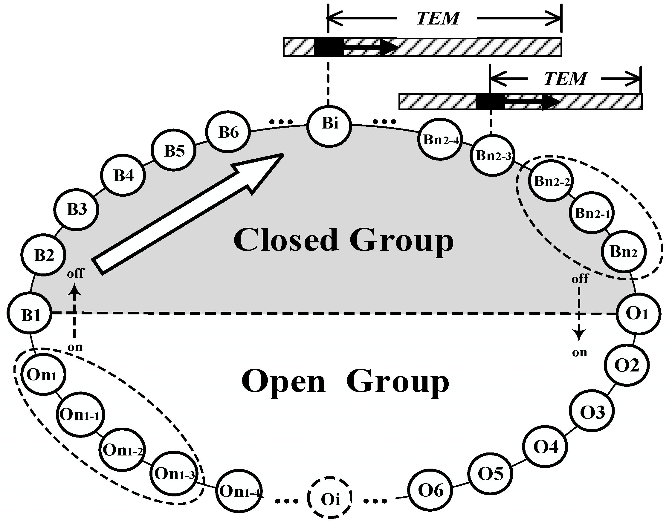
2. Modeling of Lower-Level Load Control for Central Air-conditioners Based on Comprehensive State-Queuing Model

The coordinated control algorithm is to solve an optimization problem with comprehensive constraints. A new stochastic and heuristic global optimization search method, SEUMRE is introduced in this paper. Based on the original information to predict the possible location where global solutions may exist and the direction where the search iteration times may be increased, this optimization algorithm spreads sampling points to explore the potential design space for search process. The proposed control algorithm should be applied under time-varying conditions. SEUMRE is particularly suitable for such highly nonlinear and complex optimization problems involving expensive analysis and simulation processes. Therefore, SEUMRE is chosen to calculate the optimal coordinated control demand response targets CAC group undertake.
Figure 1 gives a brief description of the optimal coordinated framework SEUMRE and IPPL method. The CAC group (CACG) is divided into two operating groups: CAC Uncontrolled Group (CACUG) and CAC Controlled Group (CACCG) based on price constraints, given optimal target and the states of terminal users at every simulation time step. An integrated-parameter-priority-list control strategy is used to generate the control command for every controlled terminal user. Taking historical switching number, current price and indoor temperature, users’ willingness, and CAC’s operating status into consideration, the integrated parameter aiming to describe the status of CAC can be determined. Although the integrated parameter will be used in a demand response scenario based on incentive mechanism, the integrated parameter also considers the constraints of pricing and other kinds of possible constraints.
The terminal users in the CACCG will update their operating state according to the command they received; the ones in CACUG will also update their state based on the established model. Then, the CACG will wait for a new optimal target that is generated from SEUMER algorithm, and update the CACUG and CACCG, which react at the next time step. In this section, the data filtering valve, detailed models of CAC that consist of CAC central unit, cooling water pump, chilled water pump, and terminal users’ temperature are presented. Electricity prices model, and switching number model are also illustrated in this part. Figure 2 depicts the relation between different detailed models of CAC.

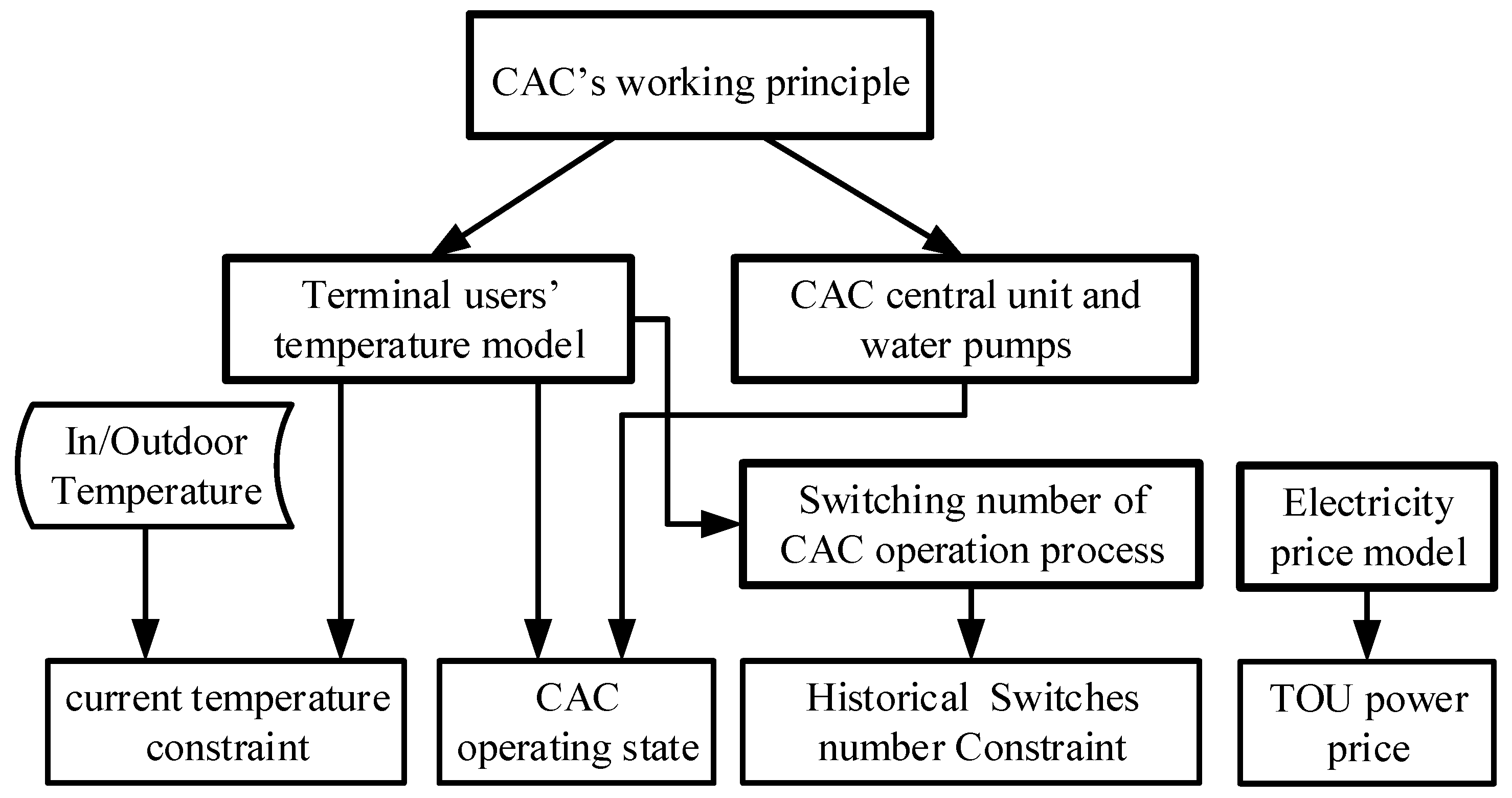
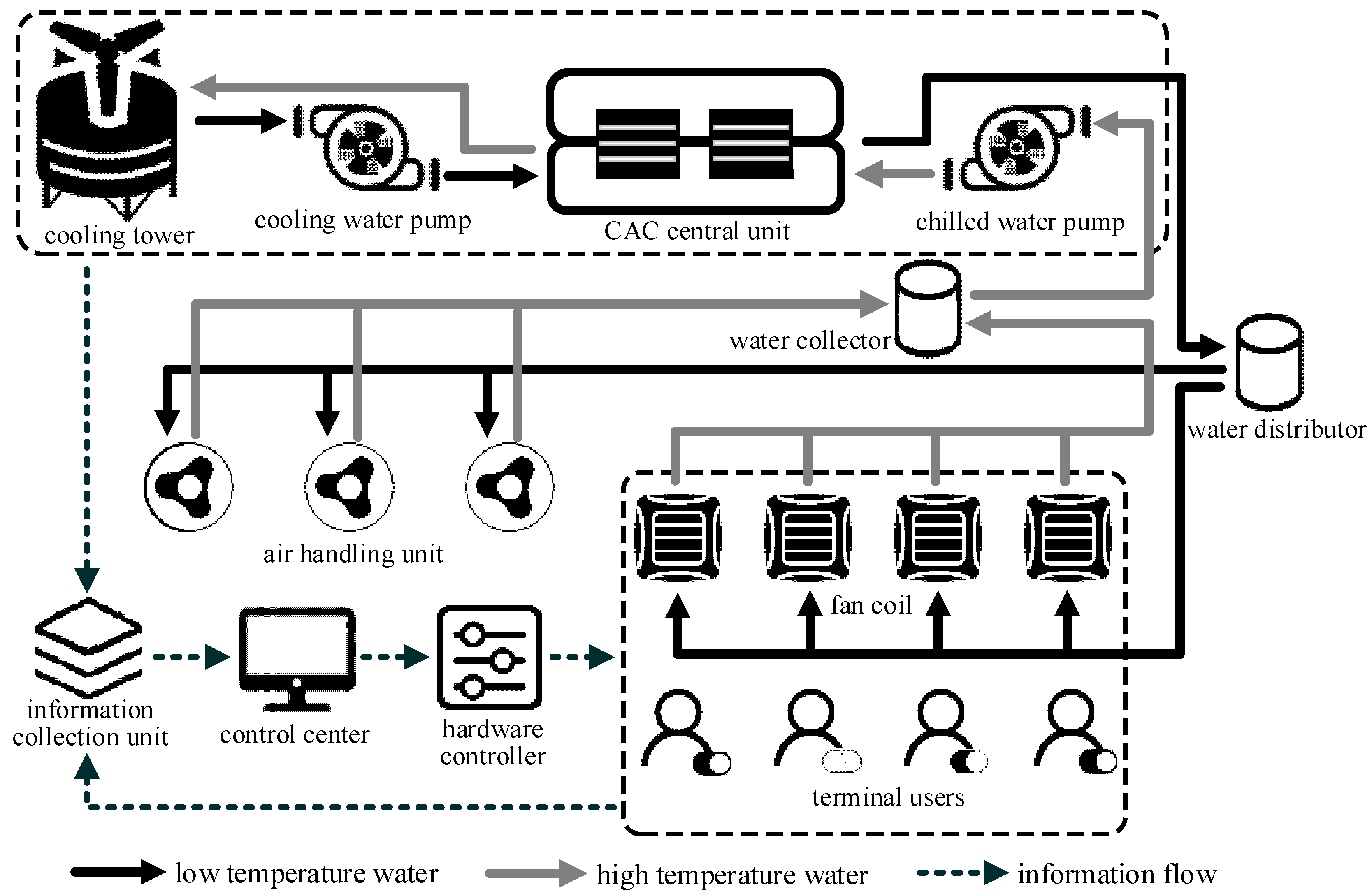
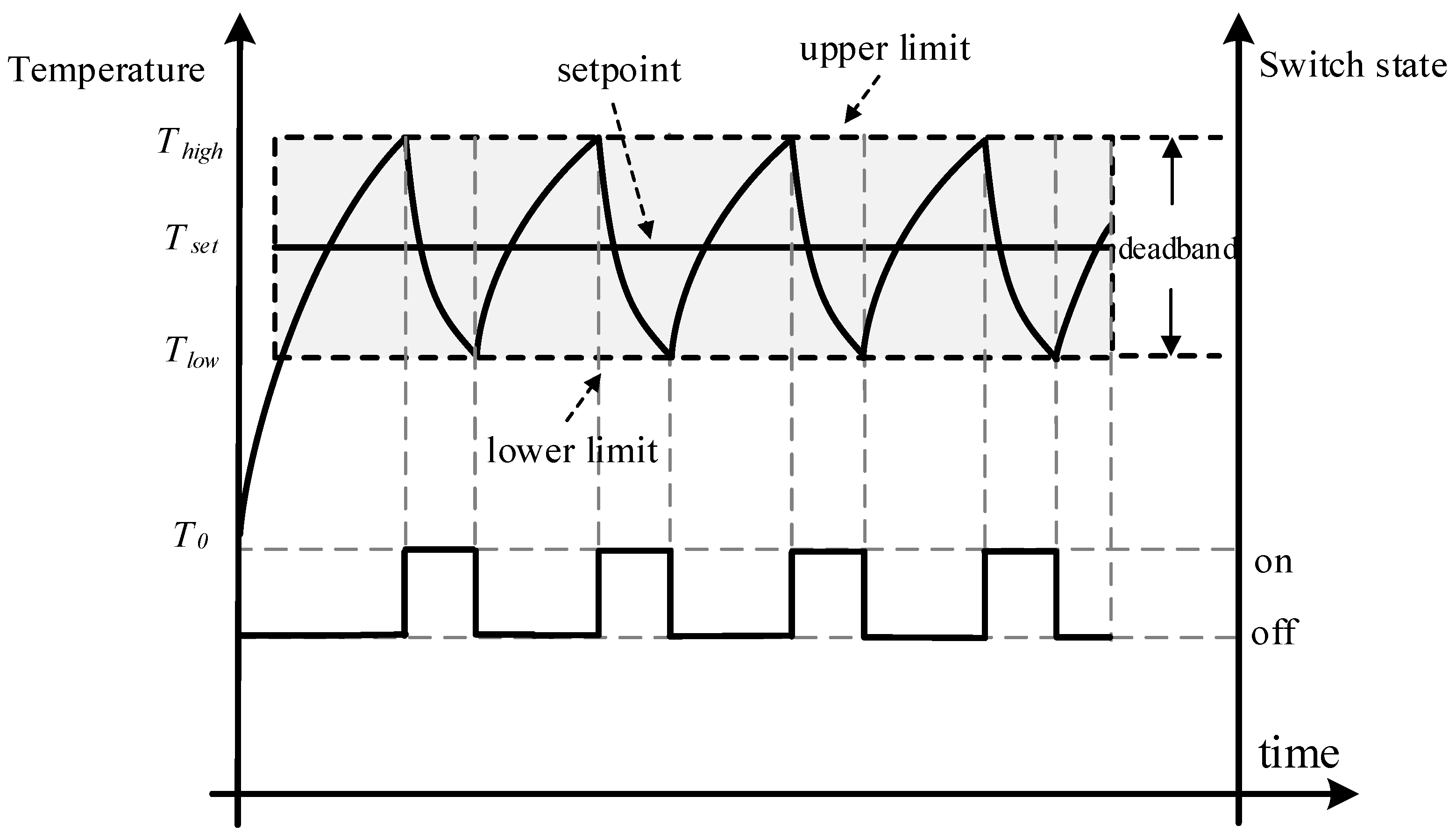
2.1. CAC’s Working Principle and Coordination Pattern with Control Strategy

Figure 3 makes detailed descriptions for the working principle of CAC and basic configuration settings when considering the controlling module added in real application. Arrows of black, gray, and dashed line represent low temperature water, high temperature water, and information flow, respectively.
The complete working process of CAC can be described as follows. A certain amount of water is chilled by CAC central units, of which the main function is heat exchange using refrigerant. The water distributer distributes the cold water to fan coil unit and air handing unit. The air handing unit is a device that is used to regulate and circulate air to improve users’ comfortable levels. Fan coil unit undertakes the task of sending cold wind to terminal users directly. The temperature of water will rise after flowing through both units. The water collector receives the water and sends it to CAC central units as heat exchange resource. The water will flow through the cooling tower, which is a heat rejection device that rejects waste heat to the atmosphere through the cooling of a water stream to a lower temperature, and it helps to reduce some power consumptions.
The information collection unit extracts CAC’s operating status and sends them to the control center in which control strategy is configured. Commands of device level are generated and are sent to the hardware controller, which forma an integrated control process.

2.2. Terminal Users’ Temperature Model of CAC

The indoor temperatures of terminal users are affected by many factors, including the switching states, setpoints, deadbands, outdoor temperatures, solar radiations, wall materials, and the output power of CAC at previous time step. When a terminal user is uncontrolled, its indoor temperature curve goes like that shown in Figure 4. Detailed descriptions of the temperature trajectory can be referred to our previous work [24]. At every time step, there are two CAC groups: open group and closed group:
O t = ( O 1 t , O 2 t , O 3 t , , O n 1 t )
B t = ( B 1 t , B 2 t , B 3 t , , B n 2 t )
where, t is the time studied, O t and B t are the open group and closed group at time t whose number of devices are n 1 and n 2 . The total number of controlled device n = n 1 + n 2 . As time goes on, n 1 and n 2 will change based on the operating status.
The whole CAC group can be defined as:
D t = ( O 1 t , O 2 t , , O n 1 t O p e n   G r o u p , B 1 t , , B n 2 t C l o s e d   G r o u p )
In this paper, the temperature difference between current value and boundary value of a device is defined as temperature extending margin (TEM) at time t:
T E M i , t = { T i , t T l o w i , t , i B t T h i g h i , t T i , t , i O t ,   i = 1 , 2 , , n
where T i , t , T l o w i , t , T h i g h i , t are the temperature of room, lower limit, and upper limit at time t. One can see that TEMs are decided by devices’ current operating status. Therefore, the devices in different group have different definitions of TEM.
Figure 5 gives an intuitive explanation of TEM. The direction from left to right represents the increase of temperature, the shadow regions show operating temperature range of devices. The locations of the black cube indicate current devices’ status and the arrow indicates the direction of temperature extending. TEMs are variable under different operative conditions. When considering the diversity and characteristic of terminal users, deadbands, and upper and lower limits of devices should also be different. At time t, a corresponding TEM set of terminal units D t :
T E M t = ( T E M 1 , t , T E M 2 , t , , T E M n , t )
The intention of introducing TEM is to provide a universal modeling method of response-control, and, finally, realize the unified response control strategies based on the concept of TEM. Through the normalization of TEM, the definition of normalized temperature extending margin (NTEM) can be given to describe the ratio of a single device’s TEM and its deadband:
N T E M i , t = { T i , t T l o w i , t δ i , t , i B t T h i g h i , t T i , t δ i , t , i O t ,   i = 1 , 2 , , n
For a controllable device, its NTEM satisfies:
0 N T E M i , t 1 , i = 1 , 2 , , n
Similarly, at time t, a corresponding NTEM set of terminal units D t . is shown in Equation (8). The normalization characteristic of NTEM is beneficial to the follow up work of control strategy design as it gives full consideration for the devices’ parameter diversities.
N T E M t = ( N T E M t , 1 , N T E M t , 2 , , N T E M t , n )
The intrinsic rule on how the devices’ temperature changes can be found in Figure 3. Two controllable groups are formed according to their switching status. NTEM can be regarded as an appropriate parameter that reflects the temperature information during the process of simulation, as it takes a full consideration of the terminal devices’ diversity, including setpoints, deadbands, and operating status.

2.3. CAC Central Unit and Water Pumps

The power consumptions of CAC central unit and water pumps account for 90% of the total power CAC needed. Similar to the model of terminal users’ temperature, many parameters have influence on the output of CAC, but most of these parameters are invariable for a unique CAC. Based on the above consideration, the time-varying parameter load ratio becomes the key factor in this model. Load ratio is a parameter that is equal to the actual refrigerated area divided by the total possible refrigerated area. To a single CAC, we calculate its power consumptions through the load ratio. This relationship is exponential like Figure 6 where load ratio varies from 0 to 1. A CAC has many terminal users, and the number of ON/OFF terminal users and the refrigerated area decided the value of load ratio.

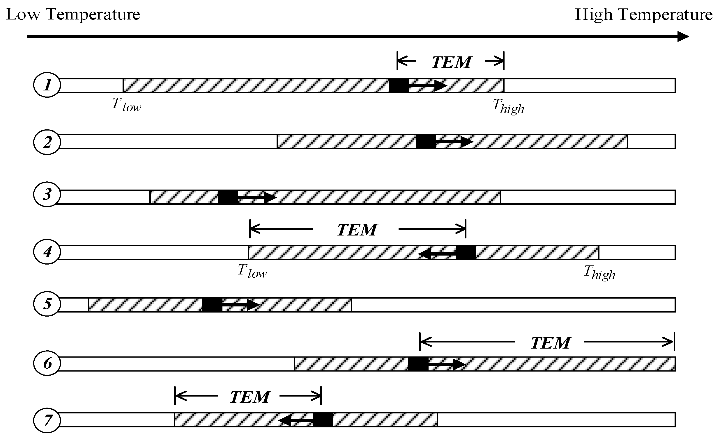
2.4. Consideration of Switching Number of CAC Operation Process

If a terminal user keeps being controlled during a long period, it may decrease the life of the device. Thus, we put up a parameter to describe the relationship between the controlled switching number and its influence. Equation (10) gives the detailed description. By adding this factor to the integrated parameter, devices could be prevented from being controlled too often. Define parameter I H S N i , t to represent the influence of historical switching number.
I H S N i , t = ( 1 H S N i t H S N _ m a x )

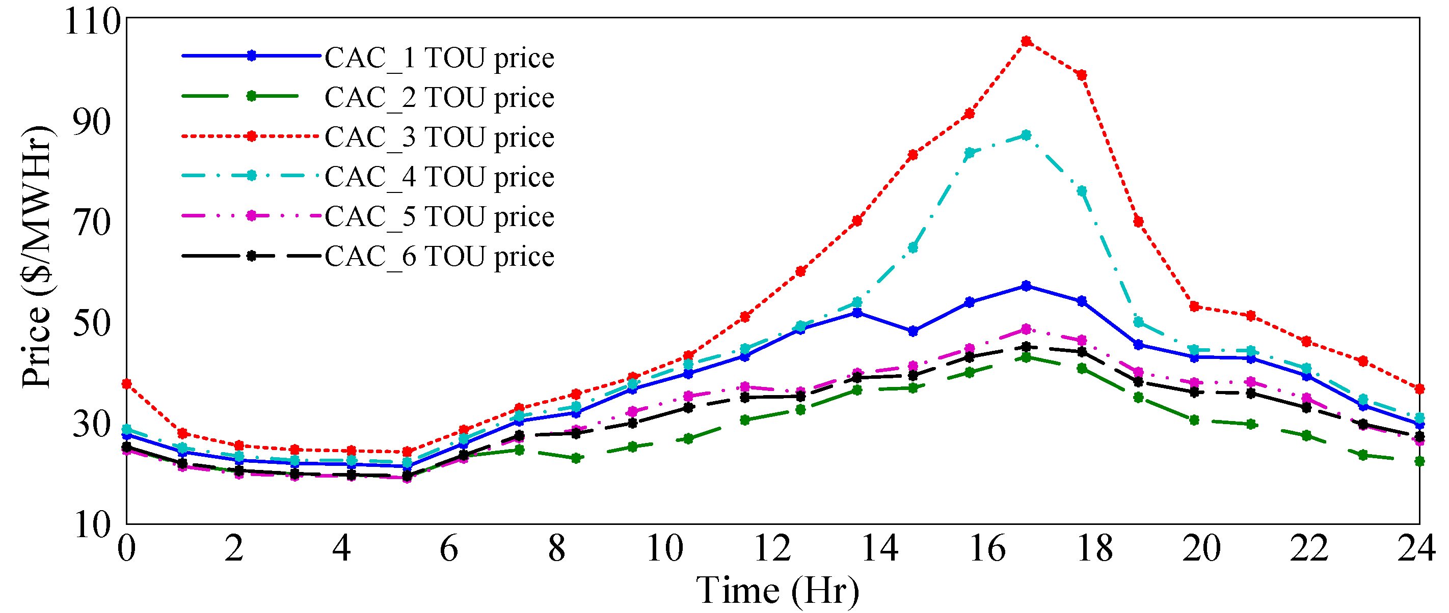
2.5. Electricity Price Model for CAC Response

In this paper, we use time of use (TOU) pricing as our price model [25]. Time of use pricing is a kind of electricity pricing strategy based on time, which can reflect power supply cost in different periods. The peak electricity price and season electricity price are two kinds of TOU price that are commonly used in China. Through setting appropriate higher electricity prices in the rush hours of a day and lower prices during the off-peak, TOU can effectively improve the users’ behavior of power using, so as to achieve load shedding effect. Figure 7 represents several typical TOU prices [25].
When assuming that the price is the same to one CAC group, that is, the users in one CAC group use the same price. If CACs are in different areas, the prices may be different. The following equation explains the influence of prices. Define parameter I P F t to represent the influence of pricing.
I P F t = 1 P r i c e t P r i c e _ max

2.6. IPPL Strategy for Comprehensive State-Queuing Model in Lower Layer

Given the target from SEUMRE algorithm, we use the IPPL strategy to generate device-level command. The original sorting rule is current indoor temperature only, but it may not be comprehensive. When considering the comfortable levels requested by users, another three parameters historical switching number, price, and users’ will to participate in demand response are introduced.
As shown in Figure 8, two controllable groups are formed according to their switching status. In each group, a number of terminal units are sorted by their NTEM, and move to the next location along the clockwise direction [24]. The intrinsic rule on how the devices’ temperature change can be found in Figure 4. As time goes, the NTEM of each device decreases continuously without any outside control in each group. This process can be seen as a constant motion in a clockwise direction.
When the temperature of a terminal unit reaches its boundary, that is, the NTEM decreases to zero, its operating status will be flipped to the opposite way, jumping from the tail of a group to the head of the other group at the next time step.
There is a positive correlation between the integrated parameter and uses’ willingness. For example, there is a load shedding requirement in winter due to a huge increase of power consumptions. In CACCG, parts of terminal users whose indoor temperatures are low, but they have strong willingness to participate in demand response. To reflect this appeal, we multiply their current indoor temperatures by the parameter I W F i , t , which is higher than other users’.
On the contrary, there is a negative correlation between the integrated parameter and historical switching number. To protect the device, switching number should be restricted in a reasonable range. For example, there is a load shedding target in winter. If a terminal user has a relatively high switching number level, we multiply the current indoor temperature by a parameter I H S N i , t , which is between 0 and 1 to decrease the possibility that it is chosen again.
For a terminal device, there is:
I i , t = ( 1 λ H S N + λ H S N I H S N i , t ) ( 1 λ T E M + λ T E M N T E M i , t ) ( 1 λ W F + λ W F I W F i , t ) ( 1 λ P F + λ P F I P F t )
The I i , t is determined by many factors, including the historical switching number, temperature of the room, users’ willing, price policy, and CAC operating status. As shown in the Equation (8), the four dimensions have played parts in the value of I i , t , and each dimension has its weighting factor λ varying from 0~100%, which is adjustable to adapt to different CAC conditions.
Replacing the order index T E M i , t with I t , the IPPL has been formed. Selecting the devices on the top of each queue based on the type of response signal, the exact number can be calculated using the stack model [24]. Finally, a group of terminal devices will be turned off or turned on. That is, CACCG decreases or increases a certain amount of power consumptions based on the types of target sent to it. In this way, device-level commands are generated. The terminal users in the CACCG will update their operating state according to the commands that they received.

3. Modeling of Upper-Level Optimal Scheduling Strategy for Aggregated Central Air-Conditioners

SEUMRE algorithm and IPPL strategy are illustrated in detail in this section. To achieve the ideal situation, we have to solve the following sub-problems, which include three aspects: the lowest cost; the best responding performance, and the best users’ comfortable levels. Each sub-problem has its own sub-problems. The best responding performance means that CACCG has accurate reaction during the controlled period and huge potential responding ability, which can be divided into two parts: load shielding ability and load rising ability. These two abilities are contradictory factors, and we try to balance them in the optimal process. The best users’ comfortable levels mean the least sacrifice of users’ living environment. We can define it as the lowest switching time and temperature adjustment. As optimization conditions are very complex, we use the intelligent algorithm SEUMRE to generate a reasonable target and IPPL strategy to generate device-level commands.

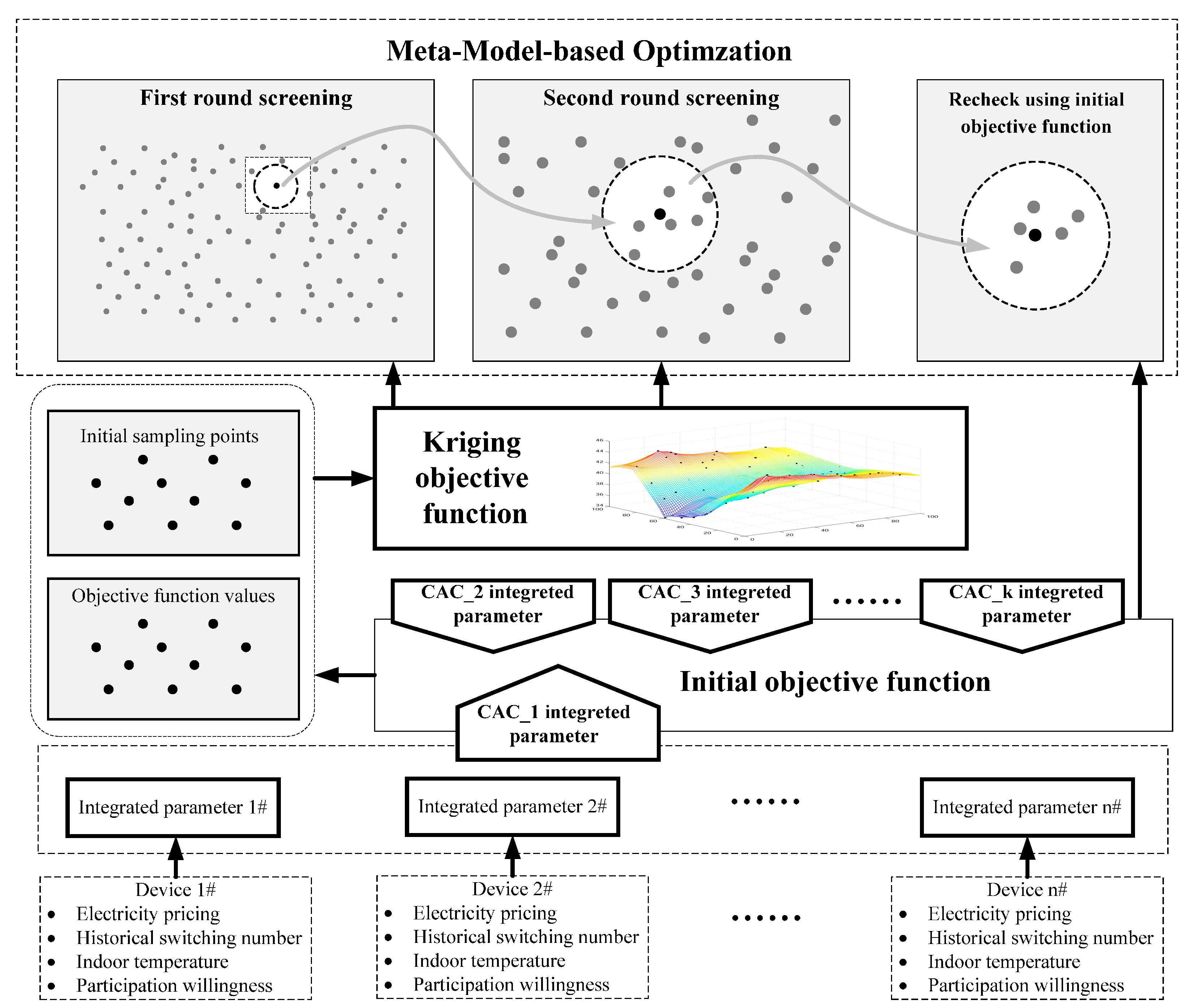
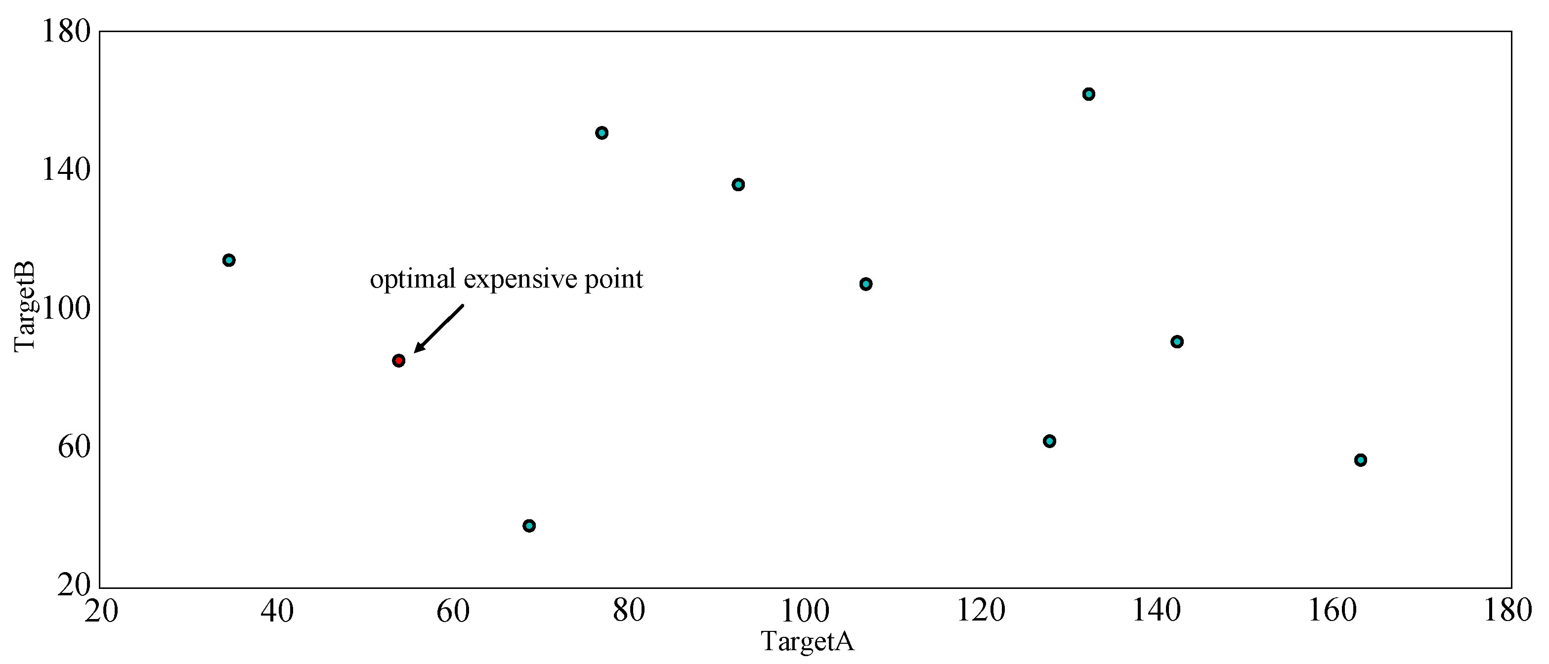
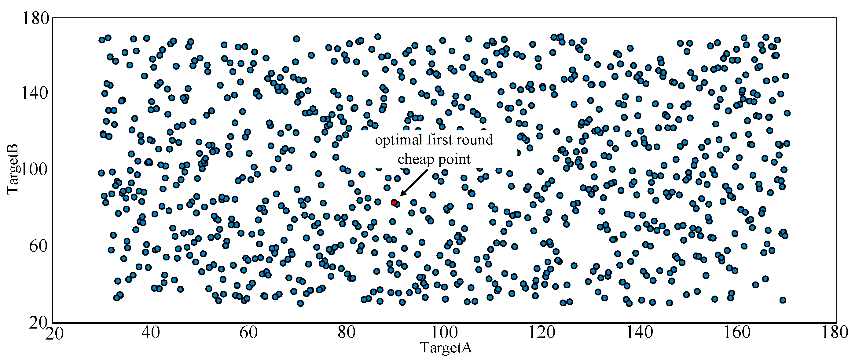
3.1. Optimization Model of Scheduling Strategy for Aggregated CAC in Upper Layer Kriging Model Based Optimization

For a single CAC, there is:
I C A C t = i = 1 n I i , t × S i S t o t a l
S t o t a l = i = 1 n S i
where S i is the cooling area of user’s room. As introduced in Section 2. The CAC’s power consumptions has a non-linear relationship with the load ratio that approximates the cooling area percent. Therefore, the I C A C t is obtained through the weighting method.
The objective function can be set according to the different simulation intentions. To make a better performance, the target distributed should be near to the natural power consumptions and avoid too much oscillation. At the start, we use the predicted power consumptions at the previous time step as the reference value, forming the objective function as follows:
Obj : min ( i = 1 m ( P t a r g e t i , t ( P C A C _ f t 1 + I C A C i , t × P o n / o f f i , t ) ) 2 )
P o n / o f f i , t = { P u p t 1 P C A C t 1 l o a d   r i s i n g P C A C t 1 P d o w n t 1 l o a d   s h e d d i n g
where, P u p t 1 and P d o w n t 1 are power limits of CAC; P o n / o f f i , t is the controllable margin of CAC. P C A C t 1 + I C A C i , t × P o n / o f f i , t stands for the ideal operating point CAC want to reach at the next time step. P C A C _ f t can be calculated by the following Equation:
P C A C _ f t = d a y = 1 m 2 m ( m + 1 ) × d a y × P C A C d a y , t 1
For historical data, the nearer days are, the more weight they should account, which has been considered in Equation (9). Figure 9 describes the flow chart of SEUMRE algorithm. By using this method, time-varying complex constraints optimization problem can be solved as long as correct configuration is set.

3.2. Space Exploration and Unimodal Region Elimination (SEUMRE) Algorithm Based on Metal Model

The key procedure of SEUMRE algorithm has the following steps:
(1)
Based on the original information, divide the designed region into several unimodal regions.
(2)
Sort the unimodal regions and predict the possible location where global solutions may exist, and the direction where the search iteration times may be increased.
(3)
Use Latin square sampling method to fit the Kriging model. Spread sampling points to explore the potential design space for search process.
(4)
First round screening: using the Kriging model, and plenty sampling points to find out the optimal point preliminarily.
(5)
Second round screening: using the Kriging model, and larger number of sampling points near the optimal point generated on step 4 to find out several optimal points.
(6)
The optimal points generated on step 5 will be rechecked with the objective function. After comparing all of the possible optimal points; we can get access to the global optimal point.
Figure 10 gives a description of the whole strategy structure. The constraints of a single device include four kinds of information: electricity pricing, historical switching number, indoor temperature, and user’s participation willingness. The constraints codetermine the integrated parameters that are different from each other. X stands for the targets needed to be calculated and distributed to the CAC response group. If there are five CAC groups, then there would be [X1, X2, X3, X4, X5] to be solved. A and B stand for the constraints matrix or vectors. To a single CAC, they are upper, lower power consumptions limits and the optimal target point, which is decided by the multi-dimension constraints. All of the parameters will be collected by the upper module, which formed the initial objective function. With the initial objective function and initial sampling points that are generated by Latin square sampling method, fitting Kriging objective function is obtained. After two rounds of screening, possible points are picked. Through rechecking and comparing the solutions using the initial objective function, we can find out the optimal point.

4. Simulation Results

In this part, several typical cases are discussed to validate the effectiveness of the strategy and the benefit brought by the application of big data. Table 1 shows the basic simulation parameters, which come from a city park in Southern China.

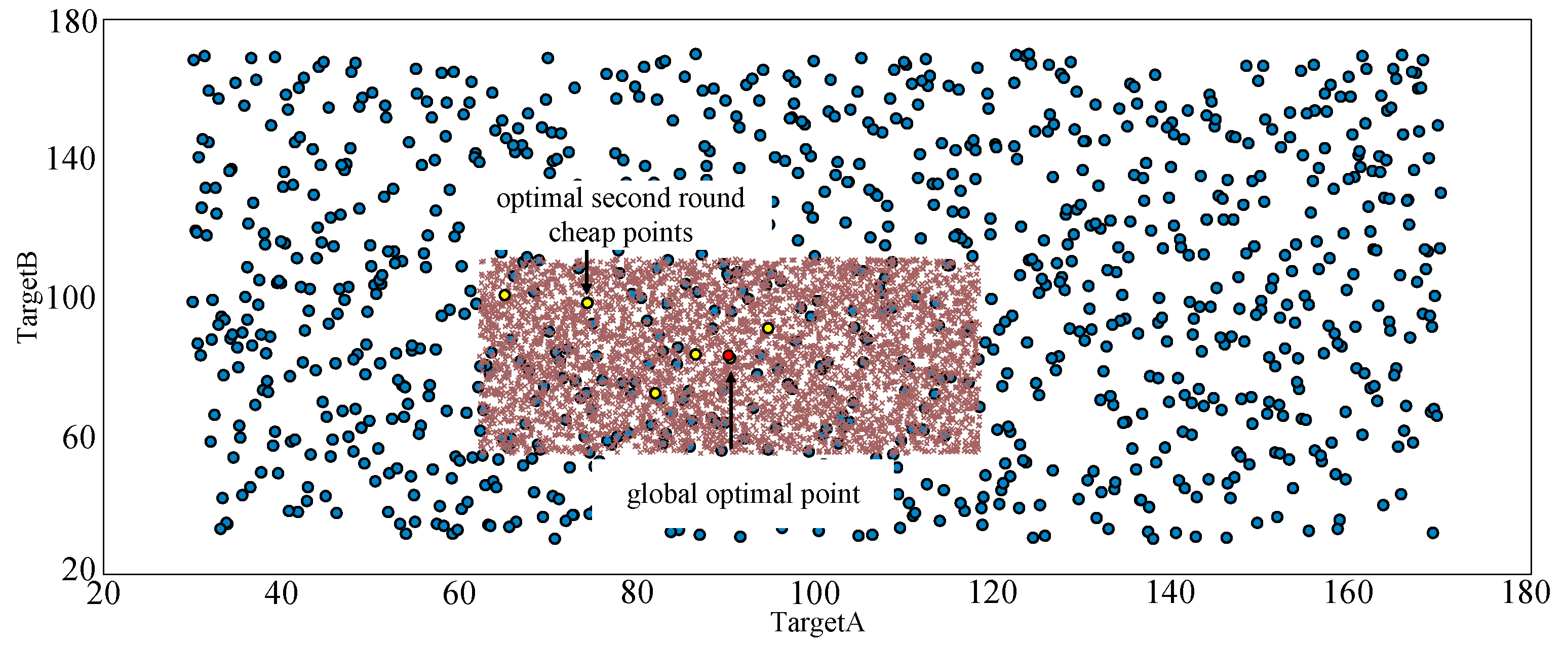
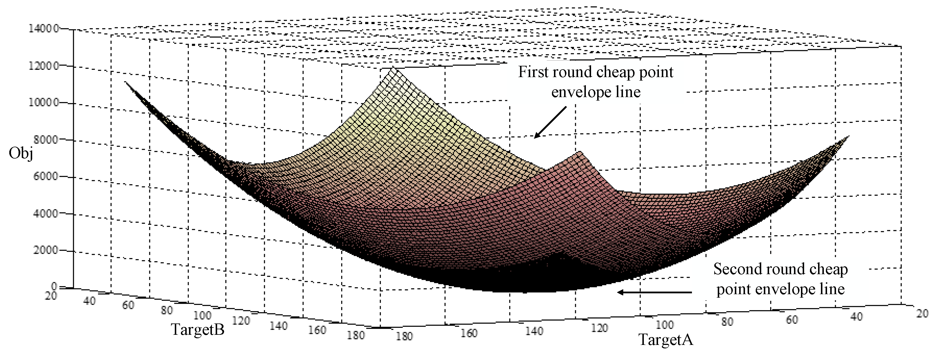
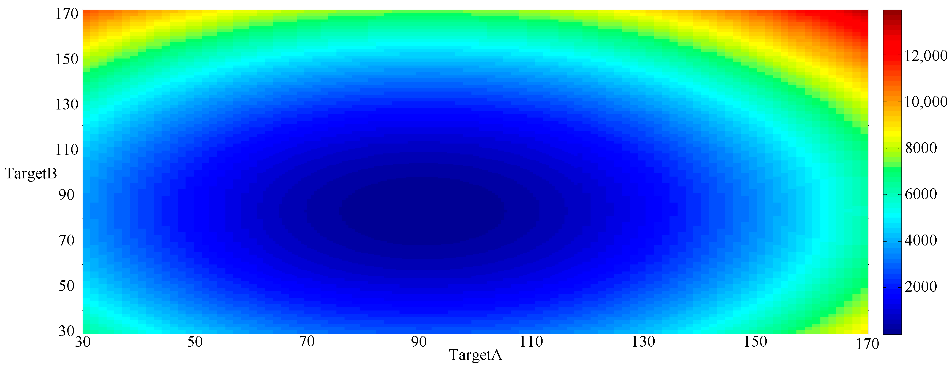
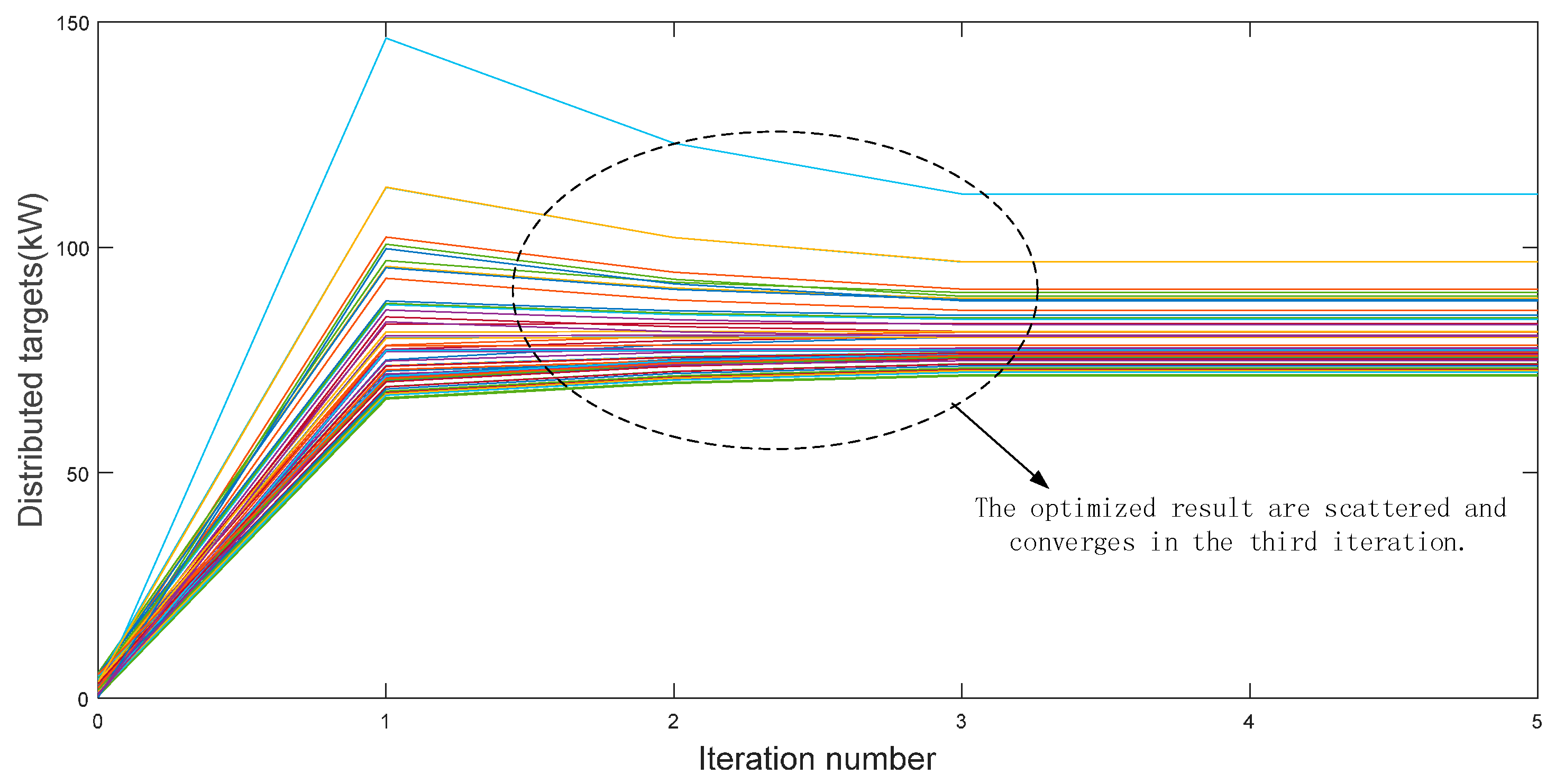
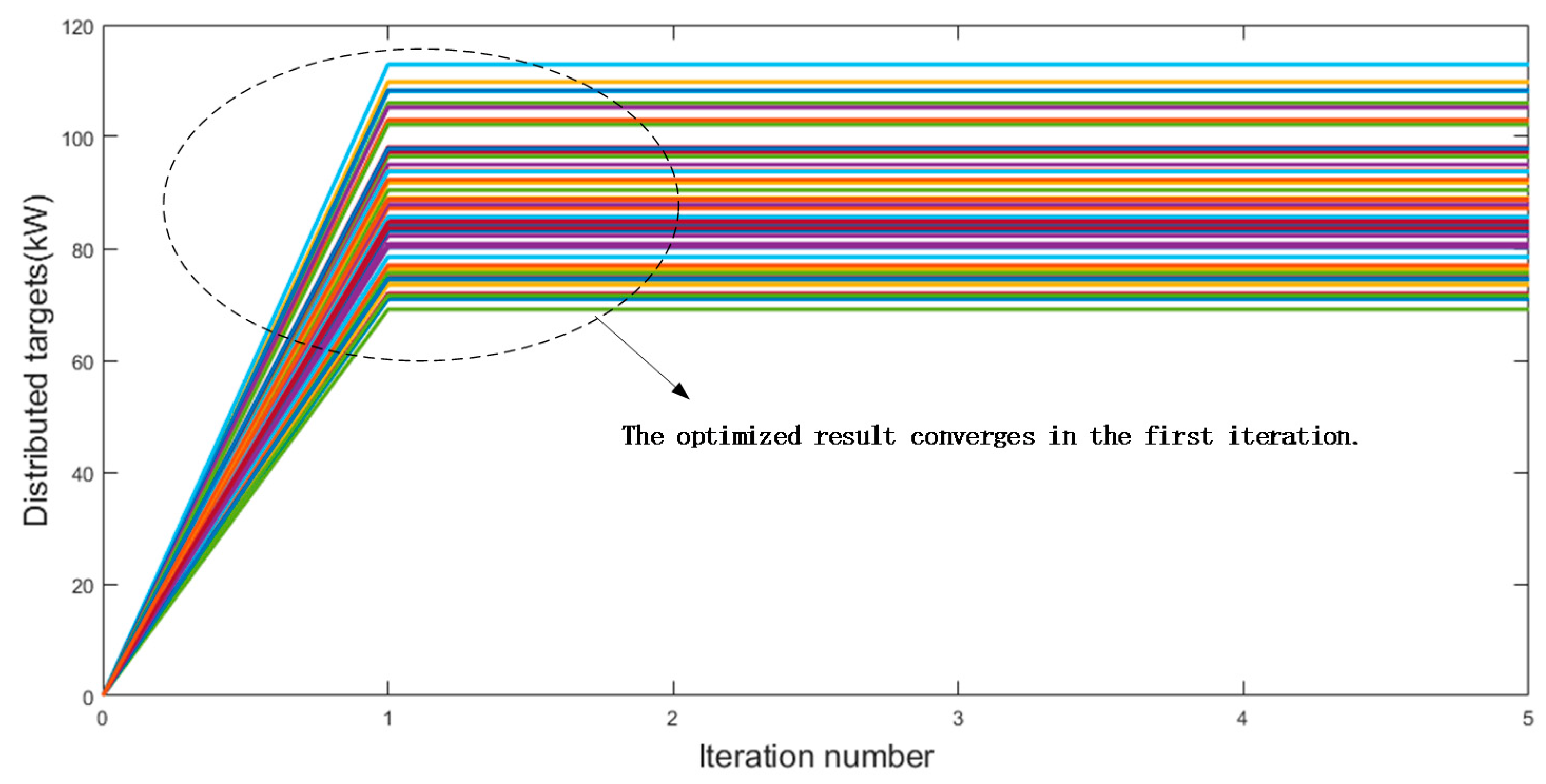
4.1. Case 1: Simulation Results of SEUMRE Algorithm

Figure 11, Figure 12, Figure 13, Figure 14 and Figure 15 will give an intuitive sense of data distribution with the SEUMRE algorithm. To make the presentation clearly, we choose only two CAC groups, A and B, which together make up the two-dimension solution space. Every point in the following figures represents a pair of target A and target B.
In Figure 11, 10 initial expensive points using the real objective function and constraint equations were tested, and we could find out the optimal expensive point dyed red. Based on the 10 initial points and corresponding objective function value, a kriging meta-model can be fitted.
In the present approach, around 1000 cheap points are generated using the metamodel, the optimal cheap point can be found dyed red in Figure 12. It is the first round cheap points screening, this optimal point in this round has already been an excellent solution.
To find a better solution, 5000 cheap points are generated using the metamodel, which has a smaller range when compared with the original sampling range. It is the second round cheap points screening with more targeted sampling points. A few solutions with minimum objective function value are chosen, dyed yellow in Figure 13. These solutions will be rechecked by the real objective function for the final verification, finding out the global optimal point dyed red in Figure 13.
The whole process can also be presented in a three-dimensional 3D and contour way. In Figure 14, target A, target B, and their objective value together make up the 3D space. The two rounds sampling points’ envelope lines are colored based on their corresponding value of objective function. The minimum value represents the global optimal solution, which can also be shown in Figure 15 as the white point.
The advantage of the SEUMRE algorithm is that it has unique method of sample points generating, which can find the optimal global points in a short time. This paper includes 60 variables using SEUMRE algorithm, all of the targets can be solved appropriately in a short time. In order to show the advantage of SEUMRE, the interior point method is used as a comparison algorithm, the SEUMRE algorithm performs better in convergence speed and optimization effect.
On the one hand, SEUMRE algorithm uses experimental data to segment the feasible field into multiple key unimodal areas, identify areas most likely to contain the global optimal solution, and use Latin square methods on these areas to fit the kriging model through additional experiments to identify the local minimum, until find the global optimal solution, which can find the optimal global points in a short time, especially in a middle-scale optimization problem, in which 50~100 variables are involved. Figure 13 shows the simulation process with 60 variables using SEUMRE algorithm, the minimum iteration step to figure out stable global optimal points reduced evidently. The simulation time is 1.6 h with 60 independent variables using the PC (Tianjin University, Tianjin, China) with CPU 2.20 GHz, i7, 4 cores, MATLAB R2013a (MathWorks, Natick, MA, USA), when compared with interior point method 6.2 h in the same machine.
From Figure 16 and Figure 17 we can see that SEUMRE only needs one iteration to get the convergence result and the interior point method need three iterations.
On the other hand, by identifying the possible unimodal regions of the objective function and reducing the search range, the SEUMRE algorithm can efficiently find the global optimal solution and avoid falling into the local optimum, so the optimized result of SEUMRE can be better than other typical optimization algorithms. The optimal solution comparison can be seen in the figure below, the target distributed by SEUMRE is nearer to the natural power consumptions than the interior point method, which can be seen in Figure 18.

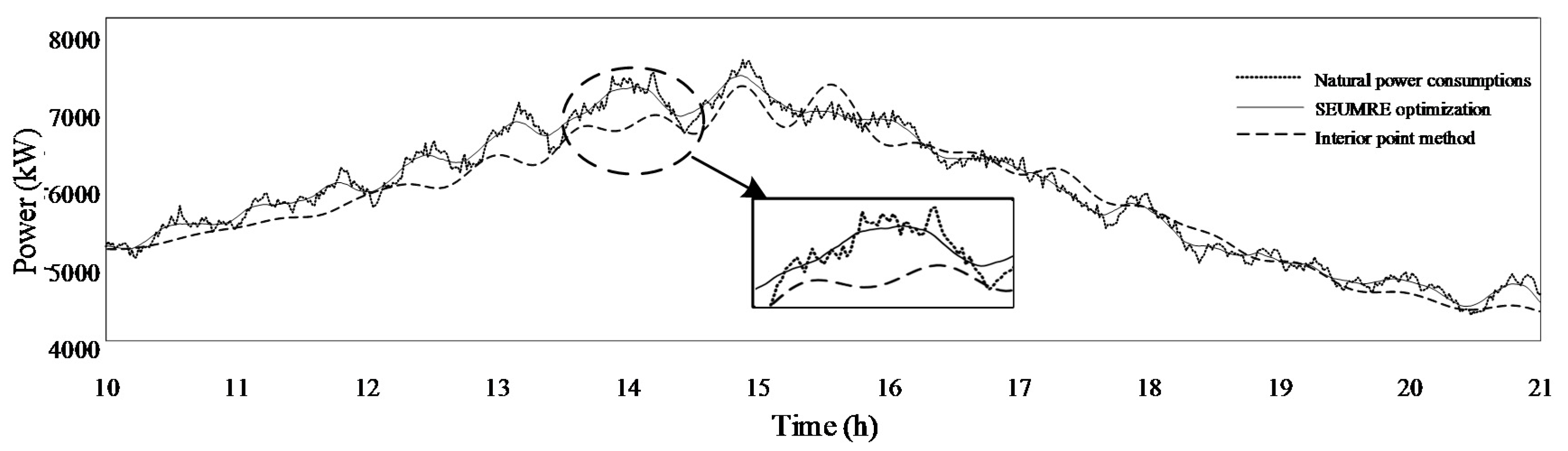
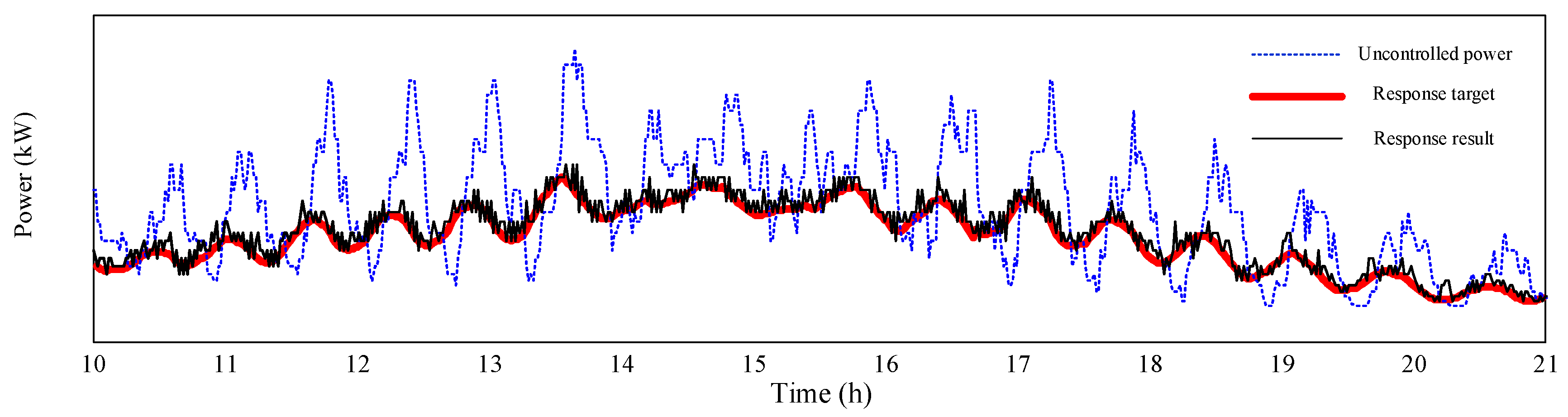
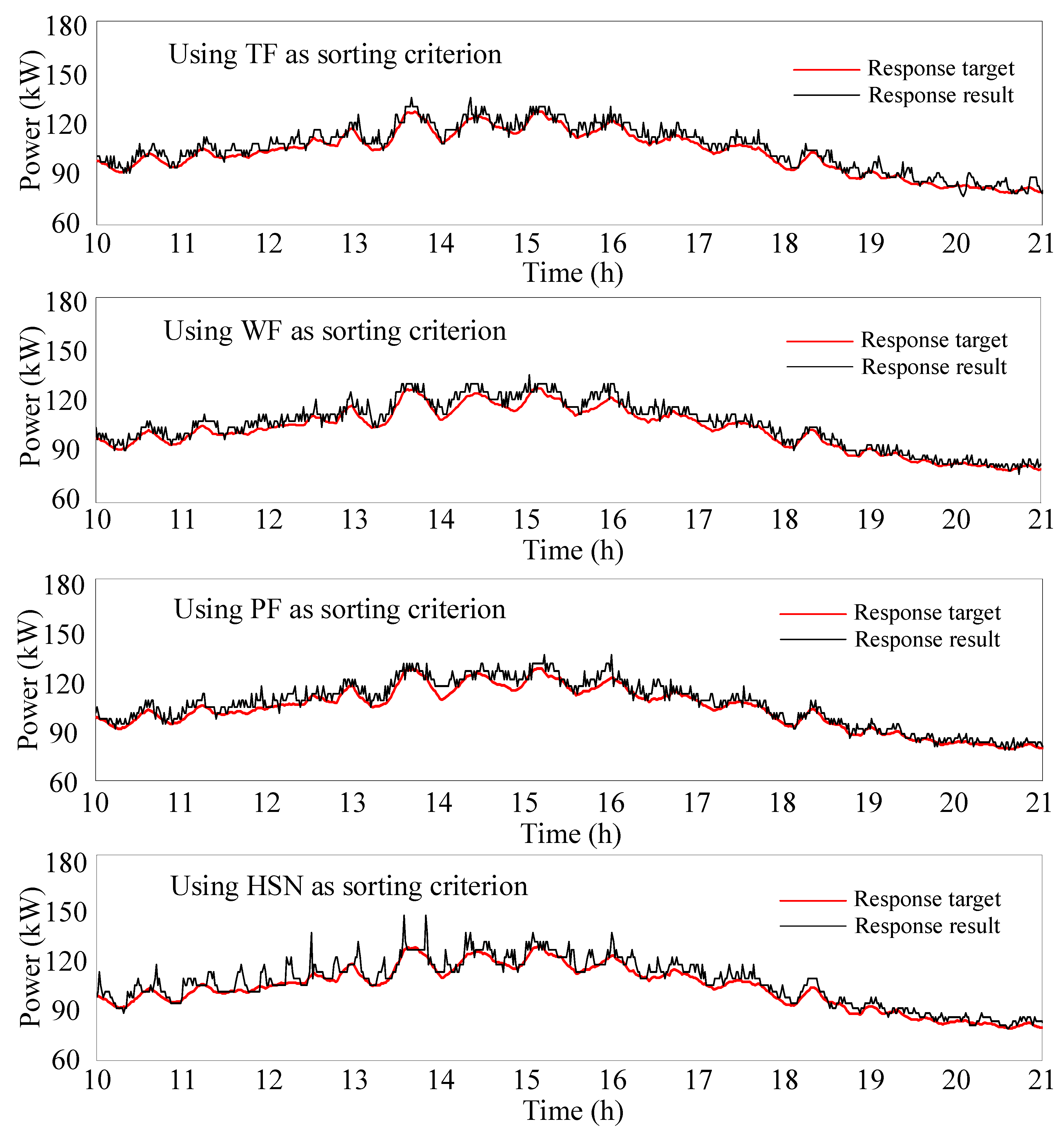
4.2. Case 2: Simulation Results of Control Strategy

Generally speaking, CAC operates during a unique time like 10 am to 9 pm. As all of the users switch on the terminal units at an approximate same time and to typical CAC user, like commercial centers, terminal rooms’ variety is not that obvious, the power consumptions of CAC will experience a period of oscillation. After simulation for a long time, like 10 days, all of the operating data have been accumulated. With the usage of historical operating data, we can forecast the power consumptions of CAC in the next day.
Through the method of smoothing, the objective points can be calculated. Figure 16 shows the response target that is generated using the Equation (14) as the objective function. When comparing to the uncontrolled power and response result, conclusions can be drawn that with the predicted objective points, power consumptions of CAC can be controlled and conducted in a smaller range with less oscillation, which can be seen in Figure 19.

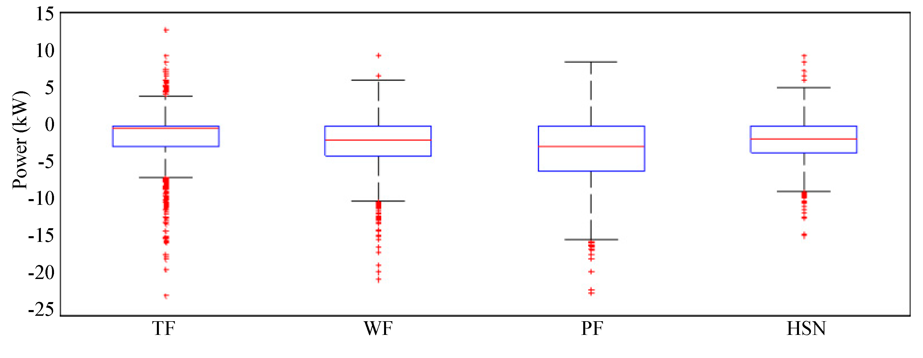
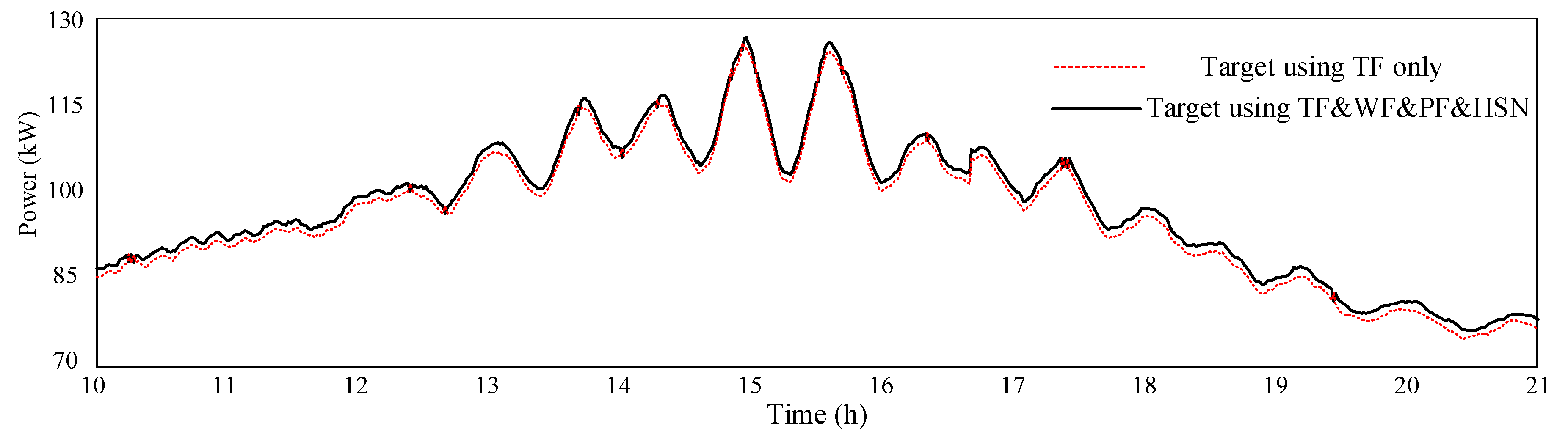
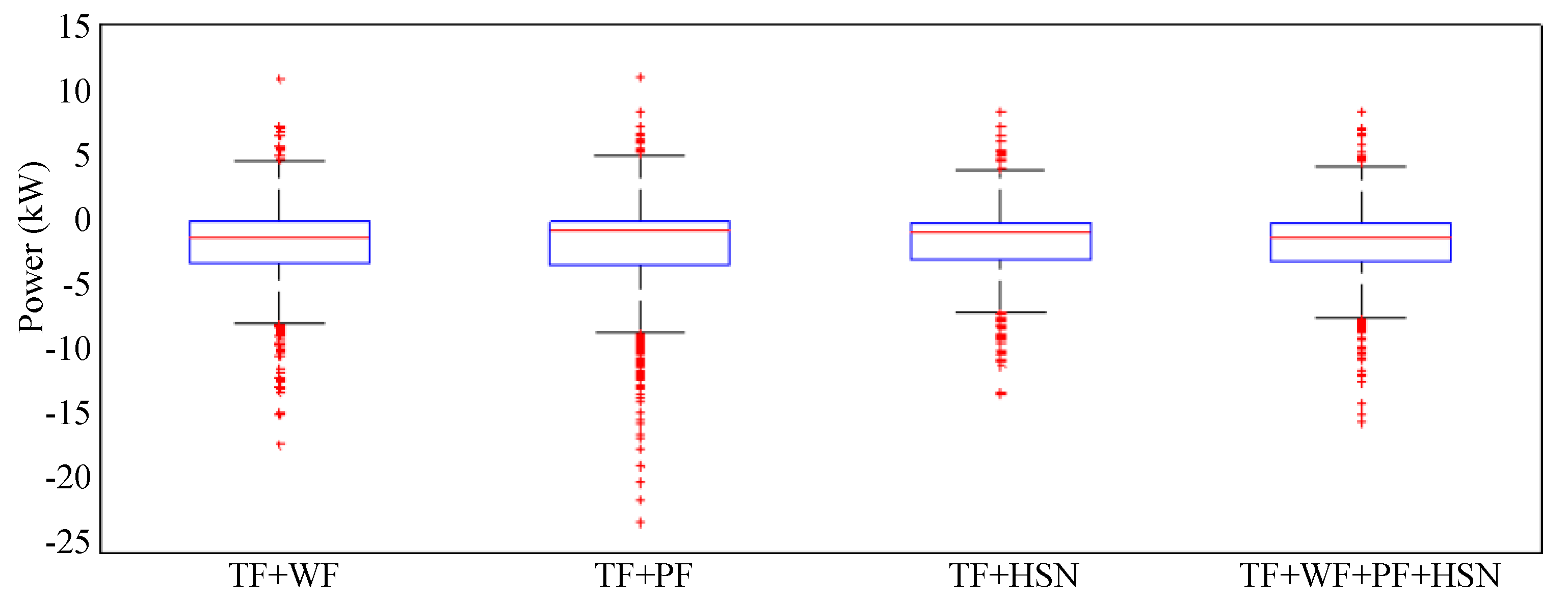
4.3. Case 3: Key Parameters of Control Strategy Analysis

In this part, four key parameters temperature factor (TF), willingness factor (WF), pricing factor (PF), and historical switching number (HSN) are analyzed. Using single parameter as sorting criterion, that is, in Equation (11), set value 1 for one of the four weighting factors λ , and 0 for the other three weighting factors. With same targets and initial conditions, four response results and errors can be obtained, as shown in Figure 20 and Figure 21.
The simulation results indicate that TF has better performance when compared to the other parameters under single sorting criterion condition. This is because temperature has its unique relationship with power consumptions, as shown in Figure 4. When temperature reaches upper or lower limits, the switching status will be changed. Although other possible parameters do not have direct connections with CAC power consumptions, they can reflect corresponding appeals in other aspects, like users’ participation willingness, pricing information, and historical switching number.
Using multiple parameters as sorting criterion, that is, in Equation (11), set value 1 for more than two of the four weighting factors λ , and 0 for the other weighting factors. When considering the importance of TF, three cases with TF and one of the other three parameters are set. The last case considers all of the possible factors, which are TF, WF, PF, and HSN. With same targets and initial conditions, four response results and errors can be obtained as shown in Figure 22 and Figure 23. The simulation results indicate that those cases when considering TF has better performance than those do not. For example, case ‘TF&WF’ has better performance than case ‘WF’ as compared with Figure 17. That is because cases considering TF take full advantages of the thermal electric coupling relationship. CAC users can set parameter weightings according to personal preferences, which realizing customization.

4.4. Case 4: Parameters’ Influence on Optimizing Target

The influences of parameters’ customization are not only on the executive part, but also on the generating of optimizing target. from Equation (14), we know that the ideal optimal point is P C A C _ f t 1 + I C A C k , t × P o n / o f f k , t , and I C A C k , t is determined by CAC users to a certain extent. Therefore, if a CAC user has larger I C A C k , t , it means the users should undertake more target (load shedding or load rising). A case of load shedding is shown in Figure 24, two targets are generated using Equation (14) colored by black and red. The target using TF&WF&PF&HSN has smaller I C A C k , t as it considers more factors, which are all in the range of 0~1. Thus, less load shedding target are distributed to it when compared with the CAC user only considering TF. By considering the parameters in the generating of optimizing target, CAC users can get reasonable targets, which match their response abilities.

5. Conclusions

This paper presents a new CAC control strategy IPPL under multiple constraints with Metal-Model-based Optimization Method and big data analysis. The simulation environment is complex and time-varying in which large amount of factors like the historical switching number, temperature of the room, users’ willing, price policy, and COP (coefficient of performance) conditions are taken into consideration, the more factors that the CAC consider, the less load shedding target would be distributed to the CAC, and the TF has better performance when compared to the other parameters. The structure in which algorithm, constraints, and models can interact effectively is presented, power consumptions of CAC can be controlled and conducted in a smaller range. The simulation results show that based on big data, with the combination of SEUMRE algorithm and IPPL strategy, CAC groups can become good candidates for demand response on the premise of accuracy and efficiency, the SEUMRE algorithm performances better in convergence speed and optimization effect, the simulation time of SEUMRE is less than 30% of the simulation time using interior point method, and the optimized result of SEUMRE is much better as the target distributed by SEUMRE is nearer to the natural power consumptions. As the optimization problem has heavy computation requirements and multi variables, in the future, more work of big data will be studied to offer auxiliary service, and help to improve the strategies.

Acknowledgments

This work was supported by National High-Technology Research and Development Program (“863” Program) of China (2015AA050403), National Natural Science Foundation of China (51407125), Shandong Province Qingdao people’s livelihood science and technology project “Research on Key Technology of Residential Renewable Energy-based Micro-grid Router”(16-6-2-60-nsh), Tianjin University independent innovation fund “Research on the key technology of distributed demand response”. The authors also would like to thank Zuoming Dong, Ning Lu, and Ned Djilali for their helpful comments and insights.

Author Contributions

Yebai Qi, Dan Wang and Yu Lan conceived and designed the study; Yebai Qi and Dan Wang performed the study; Hongjie Jia, Chengshan Wang, Kaixin Liu, Qing’e Hu and Menghua Fan reviewed and edited the manuscript; Yebai Qi wrote the paper. All authors read and approved the manuscript.

Conflicts of Interest

The authors declare no conflict of interest

Nomenclature

NotationDescription
O t Open group at time t
B t Closed group at time t
n 1 Number of devices in O t
n 2 Number of devices in B t
n Total number of controlled devices
D t The whole group at time t
T E M i , t (°C)Temperature extending margin of device i at time t
T i , t (°C)The temperature of room controlled by device i at time t
T 0 i (°C)Initial temperature of room controlled by device i
T l o w i , t (°C)Lower temperature limit of room controlled by device i at time t
T h i g h i , t (°C)Upper temperature limit of room controlled by device i at time t
N T E M i , t (pu)Normalized temperature extending margin of device i at time t
P r i c e t ($/MWh)The real-time price
P r i c e _ m a x ($/MWh)The peak price
I P F t (pu)The parameter representing the influence of pricing
H S N i t (Times)Historical switching number of device i at time t
H S N _ m a x (Times)The maximum historical switching number
I H S N i , t (pu)The parameter representing the influence of historical switching number
I W F i , t (pu)The parameter representing the influence of user’s willingness
λ H S N , λ T E M , λ W F , λ P F (pu)The parameters adjustable to adapt to different CAC conditions
S i (m2)The cooling area of user’s room
I C A C t (pu)The integrated parameter representing the CAC’s status
P t a r g e t i , t (kW)Target distributed to i th CAC
P u p t (kW)Upper power limits of CAC
P d o w n t (kW)Lower power limits of CAC
P C A C _ f t (kW)The forecasted power of CAC
TCAThermostatically controlled appliance
CACCentral air-conditioner
IPPLIntegrated parameter priority list
SEUMRESpace Exploration and Unimodal Region Elimination
DRDemand response
ESSEnergy storage system
HVACHeating, ventilation, and air-conditioner
ETPEquivalent thermal parameter
CACGCentral air-conditioner group
CACCGCentral air-conditioner controlled group
CACUGCentral air-conditioner uncontrolled group
TEMTemperature extending margin
NTEMNormalized temperature extending margin
TOUTime of use
TFTemperature factor
WFWillingness factor
PFPricing factor
HSNHistorical switching number

References

  1. Abbey, C.; Strunz, K.; Joós, G. A knowledge-based approach for control of two-level energy storage for wind energy systems. IEEE Trans. Energy Convers. 2009, 24, 539–547. [Google Scholar] [CrossRef]
  2. Heffner, G.; Goldman, C.; Kirby, B.J.; Meyer, M.K. Loads Providing Ancillary Services: Review of International Experience; LBNL-62701, ORNL/TM-2007/060; Ernest Orlando Lawrence Berkeley National Laboratory: Berkeley, CA, USA, 2007.
  3. Molina-García, A.; Bouffard, F.; Kirschen, D.S. Decentralized Demand-Side Contribution to Primary Frequency Control. IEEE Trans. Power Syst. 2011, 26, 411–419. [Google Scholar] [CrossRef]
  4. Samarakoon, K.; Ekanayake, J. Demand side primary frequency response support through smart meter control. In Proceedings of the 2009 44th International Universities Power Engineering Conference (UPEC), Glasgow, UK, 1–4 September 2009. [Google Scholar]
  5. Kirby, B.J. Spinning Reserve from Responsive Loads; ORNL/TM-2003/19; Oak Ridge National Laboratory: Oak Ridge, TN, USA, 2003.
  6. Wang, J.; Redondo, N.E.; Galiana, F.D. Demand-side reserve offers in joint energy/reserve electricity markets. IEEE Trans. Power Syst. 2003, 18, 1300–1306. [Google Scholar] [CrossRef]
  7. Behrangrad, M.; Sugihara, H.; Funaki, T. Effect of optimal spinning reserve requirement on system pollution emission considering reserve supplying demand response in the electricity market. Appl. Energy 2011, 88, 2548–2558. [Google Scholar] [CrossRef]
  8. Wang, D.; Parkinson, S.; Miao, W.; Jia, H.; Crawford, C.; Djilali, N. Hierarchal electricity market-integration of disparate responsive load groups using comfort-constrained load aggregation as spinning reserve. Appl. Energy 2013, 104, 229–238. [Google Scholar] [CrossRef]
  9. Wang, D.; Parkinson, S.; Miao, W.; Jia, H.; Crawford, C.; Djilali, N. Online voltage security assessment considering comfort-constrained demand response control of distributed heat pump systems. Appl. Energy 2012, 96, 104–114. [Google Scholar] [CrossRef]
  10. Lu, N. An Evaluation of the HVAC Load Potential for Providing Load Balancing Service. IEEE Trans. Smart Grid 2012, 3, 1263–1270. [Google Scholar] [CrossRef]
  11. Lu, N.; Zhang, Y. Design Considerations of a Centralized Load Controller Using Thermostatically Controlled Appliances for Continuous Regulation Reserves. IEEE Trans. Smart Grid 2013, 4, 914–921. [Google Scholar] [CrossRef]
  12. Callaway, D. Tapping the energy storage potential in electric loads to deliver load following and regulation, with application to wind energy. Energy Convers. Manag. 2009, 50, 1389–1400. [Google Scholar] [CrossRef]
  13. Parkinson, S.; Wang, D.; Crawford, C.; Djilali, N. Comfort-constrained distributed heat pump management. Energy Procedia 2011, 12, 849–855. [Google Scholar] [CrossRef]
  14. Parkinson, S.; Wang, D.; Crawford, C.; Djilali, N. Wind integration in self-regulating electric load distributions. Energy Syst. 2012, 3, 341–377. [Google Scholar] [CrossRef]
  15. Miao, W.; Jia, H.; Wang, D.; Parkinson, S.; Crawford, C.; Djilali, N. Active Power Regulation of Wind Power System through demand response. Sci. China (Technol. Sci.) 2012, 55, 1667–1676. [Google Scholar] [CrossRef]
  16. Lu, N.; Chassin, D.P. A state queueing model of thermostatically controlled appliances. IEEE Trans. Power Syst. 2004, 19, 1666–1673. [Google Scholar] [CrossRef]
  17. Chan, M.L.; Marsh, E.N.; Yoon, J.Y.; Ackerman, G.B.; Stoughton, N. Simulation-based load synthesis methodology for evaluating load-management programs. IEEE Trans. Power Appar. Syst. 1981, PAS-100, 1771–1778. [Google Scholar]
  18. Lin, P.I.-H.; Broberg, H.L. Internet-based monitoring and controls for HVAC applications. IEEE Ind. Appl. Mag. 2002, 8, 49–54. [Google Scholar] [CrossRef]
  19. Taylor, K.; Ward, J.; Gerasimov, V.; James, G. Sensor/actuator networks supporting agents for distributed energy management. In Proceedings of the 29th IEEE International Conference on Local Computer Networks, Tampa, FL, USA, 16–18 November 2004. [Google Scholar]
  20. Yao, L.; Lu, H.-R. A Two-Way Direct Control of Central Air-Conditioner Load via the Internet. IEEE Trans. Power Deliv. 2009, 24, 240–248. [Google Scholar] [CrossRef]
  21. Koch, S.; Mathieu, J.L.; Callaway, D.S. Modeling and control of aggregated heterogeneous thermostatically controlled loads for ancillary services. In Proceedings of the 17th Power System Computation Conference (PSCC), Stockholm, Sweden, 22–26 August 2011. [Google Scholar]
  22. Zhao, X.; Su, H.; Liu, X. Study of Control Strategy about Central Air-Conditioning Control System. In Proceedings of the Second International Conference on Information and Computing Science, Manchester, UK, 21–22 May 2009. [Google Scholar]
  23. Wakami, N.; Araki, S.; Nomura, H. Recent applications of fuzzy logic to home appliances. In Proceedings of the IECON’93 International Conference on Industrial Electronics, Control, and Instrumentation, Maui, HI, USA, 15–19 November 1993. [Google Scholar]
  24. Qi, Y.; Wang, D.; Jia, H.; Huang, R.; Zhang, Y.; Yang, Z. Demand Response Control Strategy for Central Air-conditioner Based on Temperature Adjustment of Partial Terminal Devices. Autom. Electr. Power Syst. 2015, 39, 82–88. [Google Scholar]
  25. New York Independent System Operator Official Website Public Information Page. Available online: http://www.nyiso.com/public/markets_operations/market_data/pricing_data/index.jsp (accessed on 6 March 2009).
Figure 1. Optimal Coordinated framework Space Exploration and Unimodal Region Elimination (SEUMRE) and integrated parameter priority list (IPPL) method.
Energies 10 02133 g001
Figure 2. The Relation between Detailed Models of Central Air-conditioner (CAC).
Energies 10 02133 g002
Figure 3. The working principle and basic application settings of CAC.
Energies 10 02133 g003
Figure 4. Indoor Temperature Curve of Uncontrolled Terminal User.
Energies 10 02133 g004
Figure 5. Schematic diagram of temperature extension margin.
Energies 10 02133 g005
Figure 6. Relationship of CAC’s power consumptions and load ratio.
Energies 10 02133 g006
Figure 7. CAC’s time of use (TOU) prices.
Energies 10 02133 g007
Figure 8. Schematic diagram of NTEM-based priority list.
Energies 10 02133 g008
Figure 9. SEUMRE algorithm flow chart.
Energies 10 02133 g009
Figure 10. Model solving framework.
Energies 10 02133 g010
Figure 11. Initial expensive points.
Energies 10 02133 g011
Figure 12. First round cheap points.
Energies 10 02133 g012
Figure 13. Second round cheap points.
Energies 10 02133 g013
Figure 14. Two rounds sampling points’ envelope lines.
Energies 10 02133 g014
Figure 15. Solution space in contour way.
Energies 10 02133 g015
Figure 16. 60 CACs Data distribution process with the SEUMRE algorithm.
Energies 10 02133 g016
Figure 17. 60 CACs Data distribution process with the interior point method.
Energies 10 02133 g017
Figure 18. Optimization results of 60 CAC.
Energies 10 02133 g018
Figure 19. Response result of CAC.
Energies 10 02133 g019
Figure 20. Response results under single sorting criterion.
Energies 10 02133 g020
Figure 21. Box-whisker plot of response errors under single sorting criterion.
Energies 10 02133 g021
Figure 22. Response results comparison under multiple sorting criterion.
Energies 10 02133 g022
Figure 23. Box-whisker plot of response errors under multiple sorting criterion.
Energies 10 02133 g023
Figure 24. Parameters’ influence on optimizing target.
Energies 10 02133 g024
Table 1. Basic Simulation Parameters.
CAC number60CAC‘s user number50~300
SEUMRE iteration time5Operating modecooling
Mean area of terminal units69 (m2)Mean power of CAC370 (kW)
Mean temperature setpoint of CAC21 (°C)Mean users’ will1.0
Mean temperature of upper limit24 (°C)Mean temperature of lower limit18 (°C)
Mean users’ maximum controlled switching number20/dayMean users’ maximum total switching number80/day
Simulation step (min)1Simulation time (day)15
Simulation start time every day (min)600Simulation time every day (min)1260

