Chance-Constrained Real-Time Dispatch with Renewable Uncertainty Based on Dynamic Load Flow

Abstract

In this paper, a comprehensive real-time dispatch model considering renewable uncertainty based on dynamic load flow (DLF) is proposed. Through DLF, the primary and secondary frequency regulation amount caused by the variation of renewable energy as well as the line flow when primary and secondary regulation are deployed can be obtained easily. Not only the frequency constraints, but also the regular constraints like generator production limits and line flow limits are respected under both primary and secondary frequency regulation. To solve the dispatch problem with renewable uncertainty, chance-constrained programming based on cumulants and Cornish-fisher expansions (CCP-CMCF) is adopted to get the probability of holding the chance constraints and then the real-time dispatch model can be transformed into a quadratic programming. The simulation results show that the dispatch model proposed in this paper can deal with both primary and secondary regulation well and has a fast computation speed.

1. Introduction

Power systems have been undergoing a significant increase in renewable energy penetration over the past decades. Their volatility and unpredictable nature, however, make large-scale integration of these renewable sources challenging. Moreover, large fluctuations of wind power in a short time period, such as significant increases or decreases will also cause system frequency fluctuations, which threaten the reliability and security of power system operation.

Some researchers have explored the issue of maintaining the power balance in power dispatch. In [1], spinning reserve of conventional generators was required to be larger than a certain percentage of wind generation in case of a shortage or spillage of wind power, but this kind of formulation doesn’t quantify the exact amount of the reserve and may cause inaccurate results. An affine adjustment of automatic generation control (AGC) units is applied in [2,3], in which all unbalanced wind power is allocated by AGC units with their participation factor, but it only considers the secondary regulation of frequency. The authors of [4] proposed a formulation for frequency constraints from the point of kinetic energy, but it cannot consider the transmission constraints during the primary control. In [5,6], a reverse and forward engineering approach is applied to develop the AGC scheme to achieve economic efficiency, but the primary constraints are not considered. In [7], a unit commitment problem is presented to minimize the overall cost of generation and of supplying both tertiary and primary reserve services over the scheduling horizon, however, the renewable energy is not taken into consideration.

As mentioned in [8], increased variable renewable generation will have an impact on the adequacy of primary reserves, and primary frequency control may lead to transmission bottlenecks that prevent effective delivery of primary frequency control, so it is important to include the primary regulation into any dispatch model of a power system with renewable energy integration.

In fact, it is difficult for the system frequency to stay unchanged due to the volatility of renewable energy. All generators with speed controller output will adjust automatically according to their power-frequency characteristics, while all AGC units’ reference outputs are adjusted by the secondary control. Hence, it is improper to treat frequency as a constant parameter, and primary and secondary regulation should be considered carefully to accurately simulate the operation of a real power system. To quantify the primary and secondary frequency regulation amount of generators, dynamic load flow (DLF) is introduced in this paper. With DLF, first proposed in [9], generator-demand unbalanced power is allocated among all generators with speed controllers, but this model cannot obtain the system frequency. In [10,11], the steady-state frequency is taken as an unknown variable in DLF computation. Reference [12] applied DLF to simulate the plunge and upsurge of wind power, and showed that the power flow results obtained by DLF can be more accurate when the injected power fluctuates, but the uncertainty of wind energy should also be considered in DLF in modern power systems.

Regarding the uncertain optimization, there are three commonly used models to solve the optimization problem of power systems considering uncertainty, i.e., robust optimization (RO) [2,3,13,14,15,16,17], stochastic programming (SP) [4,18,19] and chance-constrained programming (CCP) [20,21,22]. The RO approach seeks to optimize system performance by finding the solution that can deal with the worst case. SP models take advantage of the fact that probability distributions governing the data are known or can be estimated. In general, RO focuses on the worst case, which may lead to over-conservative results, as the probability that the worst case will happen may be extremely small. SP can produce more economic results, however, it usually has more computational burden.

CCP is an alternative to solve the economic dispatch under uncertainty conditions. As mentioned in [16], the inequality constraints in a power system are not rigid but soft ones, which means that exceeding the boundary limits by a little may be permissible. Thus, CCP can be a useful tool to evaluate the probability or reliability of holding boundary constraints. However, it is difficult to get the probability of holding the constraints in economic dispatch. Some references have explored this problem.

The authors of [20] came up with a framework including a simulation layer and an optimization layer to solve the optimal power flow (OPF) under uncertainty. A back-mapping approach is implemented to obtain the probability of holding an output constraint, but the back-mapping approach presented is not accurate. Reference [21] formulates a stochastic optimization program with chance constraints. In order to solve the chance constrained problem, the authors propose to use the scenario approach to calculate the uncertainty bounds and then transform the problem into a robust one. In addition, a Quantile-Based approach is also mentioned in this paper, in which the wind power is treated as a bounded uncertainty, with the bounds corresponding to two extreme cases. The simulation results show that the solution given by scenario approach is more conservative than that given by Quantile-Based approach. However, there is only one wind farm in the model, which means the approach is not suitable for power systems that have more than one wind farm. Different analytic reformulations for chance constraints are discussed in [22] and it is pointed out that the reformulated chance constraints all have a similar form, but this approach cannot make full use of the distribution properties and may be inaccurate. Reference [23] developed a method dealing with random variables using Gaussian mixture model (GMM), which can deal with the irregular distribution well, but it has to use an iteration method to obtain the inverse of cumulative distribution function (CDF), which may influence the computation time. In order to overcome the drawbacks of the existing methods of calculating the probability of holding constraints, we propose a chance-constrained programming based on Cumulants and Cornish-fisher expansion (CCP-CMCF) to solve the real-time dispatch with renewable uncertainty and frequency regulation, in which the cumulants of random variables and Cornish-fisher expansions are adopted to calculate the probability of holding chance constraints. Thus, the model can be reformulated as a quadratic programming. This approach is suitable for many distributions, as long as the moments of the distribution exist and the density function is continuous. The main contributions of this work are as follows:

• DLF is developed in this paper, through which the primary and secondary frequency regulation amount caused by the variation of renewable energy can be obtained as well as the line flow when primary and secondary regulation is deployed.
• A comprehensive real-time dispatch model based on DLF is proposed in this paper, in which the frequency constraints, line flow limits, generation production limits are respected under both primary and secondary frequency regulation.
• CCP-CMCF is adopted in our real-time dispatch model, in which cumulants and Cornish-fisher expansions are adopted to get the probability of holding the chance constraints and then the real-time dispatch model can be transformed into a quadratic programming. Moreover, the spatial and temporal correlation of renewable sources is carefully modeled and evaluated on the dispatch results.

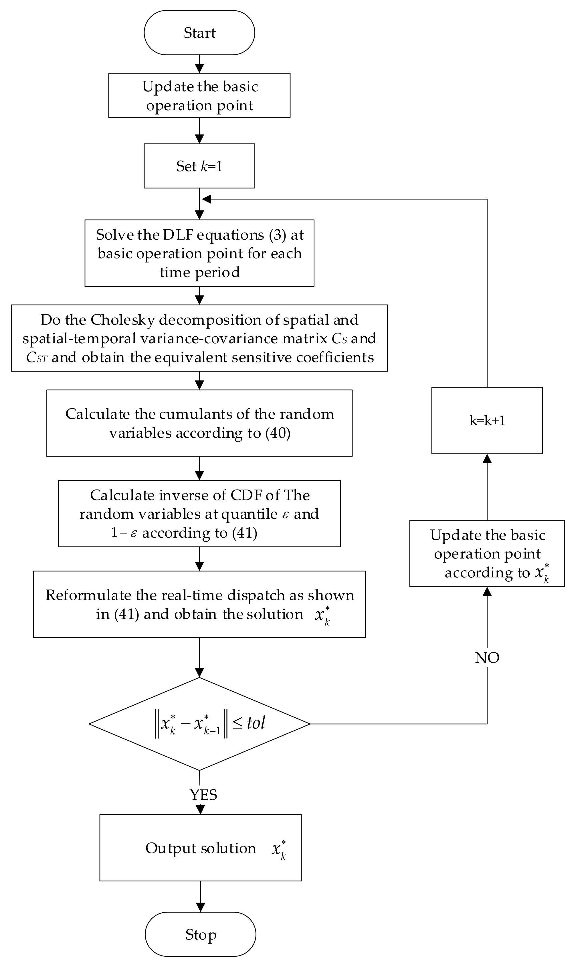
The rest of this paper is as follows: Section 2 introduces DLF and frequency regulation caused by renewable energy variation. Section 3 gives the mathematical formulation of real-time dispatch. Section 4 introduces the cumulants of random variables and Cornish-fisher expansion and then reformulates the model proposed in Section 3. The solving procedure is presented in Section 5 and the model is tested in Section 6. Section 7 gives our conclusions.

2. DLF and Frequency Regulation of Power System with Respect to Renewable Energy

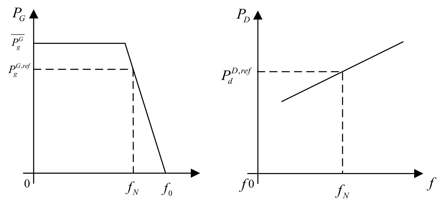
Frequency regulation can be classified into primary, secondary, and tertiary regulation according to its response time and its regulation mechanism. Primary regulation is provided by the generating units through their droop characteristic in response to system frequency deviations, which is the fastest among the three kinds of regulation. Secondary regulation, also known as AGC, is a centralized strategy whose goal is to regulate the area-control error under load-following conditions. All generator units with speed governors operating in a power system contain stored kinetic energy due to their rotating masses. When the imbalance between demand and generation arise, the system frequency deviates from its reference point as the kinetic energy of the rotating masses changes, which is also called the droop characteristic. The steady-state power-frequency relation can be expressed as [12,24]:

$$P_g^G=P_g^{G,ref}-K_g^G(f-f_N), g\in G$$

(1)

where $K_g^G$ is the generator frequency regulation constant or governor droop of unit g.

The active load has the similar expression [12]:

$$P_d^D=P_d^{D,ref}+K_d^D\left(f-f_N\right), d\in D$$

(2)

The power-frequency relation of generators and load are shown in Figure 1.

2.1. DLF Model

To quantify the primary and secondary frequency regulation amount of generators, DLF is introduced. When renewable energy output deviates from the forecast value, the power output of generators will change according to their droop characteristic, which also influences the line flow.

The load flow model considering primary regulation can be expressed as (3) and (4), in which the steady-state frequency f is also a state variable:

$$\{\begin{array}{l}{P}_i=V_i{\displaystyle \sum _{j=1}^n{V}_j(G_{ij}\cos {\theta }_{ij}+B_{ij}\sin {\theta }_{ij})}, i=1,2,\cdots ,n\\ Q_i=V_i{\displaystyle \sum _{j=1}^n{V}_j(G_{ij}\sin {\theta }_{ij}-B_{ij}\cos {\theta }_{ij})}, i=1,2,\cdots ,m\end{array}$$

(3)

$$P_i={\displaystyle \sum _{g=1}^{Ng,i}\left(P_g^{G,ref}-K_g^G(f-f_N)\right)}-{\displaystyle \sum _{d=1}^{Nd,i}\left(P_d^{D,ref}+K_d^D\left(f-f_N\right)\right)}+{\displaystyle \sum _{w=1}^{Nw,i}{\tilde{P}}_w^W}, i=1,2,\cdots ,n$$

(4)

Note that the active injection power of slack bus is also included. Hence, the number of equations and the number of unknown variables are still the same, which means it is solvable.

The correction function is:

$$\left[\begin{array}{c}\mathsf{\Delta }P\\ \mathsf{\Delta }Q\\ \mathsf{\Delta }{P}_n\end{array}\right]=J_D\left[\begin{array}{c}\mathsf{\Delta }\theta \\ \mathsf{\Delta }V\\ \mathsf{\Delta }f\end{array}\right]=\left[\begin{array}{ccc}H& N& C\\ K& L& \\ H_n& N_n& C_n\end{array}\right]\left[\begin{array}{c}\mathsf{\Delta }\theta \\ \mathsf{\Delta }V\\ \mathsf{\Delta }f\end{array}\right]$$

(5)

The elements of $C$ (including $C_n$) reflect the frequency regulation constant of generators and load:

$$C_i=\{\begin{array}{l}{\displaystyle \sum _{g=1}^{Ng,i}{K}_g^G}-{\displaystyle \sum _{d=1}^{Nd,i}{K}_d^D}, i\mathrm{is}\mathrm{generator}\mathrm{bus}\\ -{\displaystyle \sum _{d=1}^{Nd,i}{K}_d^D}, i\mathrm{is}\mathrm{load}\mathrm{bus}\\ {\displaystyle \sum _{g=1}^{Ng,n}{K}_g^G}-{\displaystyle \sum _{d=1}^{Nd,n}{K}_d^D}, n\mathrm{is}\mathrm{slack}\mathrm{bus}\end{array}$$

(6)

Renewable energy forecast error can be considered as a random variable. When the error is not large, the modified power flow Equation (3) can be Taylor expanded near the basic operation point:

$$\begin{array}{l}X\approx X_0+\mathsf{\Delta }X=X_0+S\mathsf{\Delta }W\\ Z\approx Z_0+\mathsf{\Delta }Z=Z_0+T\mathsf{\Delta }W\end{array}$$

(7)

The sensitivity coefficient matrixes $S,T$ can be obtained by:

$$\{\begin{array}{l}S=J_D^{-1}\\ T=G_{br}S\end{array}$$

(8)

2.2. Primary Frequency Regulation

Since primary regulation responds fastest (usually within several seconds), it is necessary to evaluate the primary regulation amount of generators. With the help of DLF, the frequency deviation caused by renewable power variation can be expressed as:

$$\Delta f={\displaystyle \sum _{w=1}^{Nw}{S}_w^{fw}\Delta {\tilde{P}}_w^W}$$

(9)

The primary regulation amount of generator g is:

$${\tilde{r}}_g^P=-K_g^G{\displaystyle \sum _{w=1}^{Nw}{S}_w^{fw}\Delta {\tilde{P}}_w^W},g\in \left\{1,2,\cdots ,Ng\right\}$$

(10)

Define $S_{gw}^P=-{\displaystyle \sum _{w=1}^{Nw}{K}_g^G{S}_w^{fw}}$ as the primary regulation coefficient of generator unit g with respect to renewable source w.

In a matrix form:

$${\tilde{R}}_{}^P=S_{}^P\Delta \tilde{W}$$

(11)

If primary regulation is insufficient, the system frequency may suffer severe deviation due to sudden change of renewable energy before secondary regulation is deployed.

2.3. Secondary Frequency Regulation

As shown in Section 2.2, there is a steady-state frequency error in primary regulation when the change in reference setting is zero. In secondary regulation (also called AGC), the steady-state frequency error should be restored to zero, usually within one minute. To achieve this, the secondary regulation of AGC units should satisfy:

$${\displaystyle \sum _{g=1}^{Ng}{S}_g^{fg}{\tilde{r}}_g^S}+{\displaystyle \sum _{w=1}^{Nw}{S}_w^{fw}\Delta {\tilde{P}}_w^W}=0$$

(12)

Note that the AGC units’ regulation amount is decided by their participation factor a_g. Therefore, the secondary regulation amount of generator g can be expressed as:

$${\tilde{r}}_g^S=-{\alpha }_g\frac{{\displaystyle \sum _{w=1}^{Nw}{S}_w^{fw}\Delta {\tilde{P}}_w^W}}{{\displaystyle \sum _{g=1}^{Ng}{S}_g^{fg}{\alpha }_g}},{\displaystyle \sum {\alpha }_g}=1,$$

(13)

Define $S_{gw}^S=-\frac{{\displaystyle \sum _{w=1}^{Nw}{S}_w^{fw}{\alpha }_g}}{{\displaystyle \sum _{g=1}^{Ng}{S}_g^{fg}{\alpha }_g}}$ as the secondary regulation coefficient. We don’t distinguish AGC units and non-AGC units in this paper. Instead, we just need to set the participation factor of non-AGC units to be zero. The matrix form of (12) is:

$${\tilde{R}}_{}^S=S_{}^S\Delta \tilde{W}$$

(14)

3. Chance-Constrained Real-Time Dispatch Model

The real-time dispatch aim is to determine all committed generators’ output (reference point of non-AGC units and set point of AGC-units) in a receding horizon every 5 min in the coming hour. Each real-time dispatch schedule is composed of 12 points. Between the adjacent dispatch points, the reference point of non-AGC units will be locked and their actual power output will change according to their droop characteristic if active power mismatch happens. Meanwhile the AGC units will also adjust their reference output, but the response time is much longer than primary regulation.

To ensure the sufficiency of both primary and secondary regulation amount and also the security and reliability of power system operation under both regulations, we point out that all generators with speed governors should provide primary regulation reserve to deal with the sudden increase or decrease of renewable energy, meanwhile the transmission line flow limits should not be violated to make sure that the primary regulation can be delivered through the network.

The objective function is to minimize the total operation cost:

$$\min {\displaystyle \sum _{t=1}^T\left\{{\displaystyle \sum _{g=1}^{Ng}\left(a_g\cdot {\left(P_{g,t}^{G,ref}\right)}^2+b_g\cdot P_{g,t}^{G,ref}+c_g\right)}\right\}}$$

(15)

Constraints:

(1) Frequency constraint

Instead of power balance equation in conventional dispatch model, frequency constraint is respected in our model. The frequency should not violate the lower and upper limit under primary regulation, and should be rated frequency value under secondary regulation:

$$\{\begin{array}{l}\underset{\_}{f}\le {\displaystyle \sum _{g=1}^{Ng}{S}_{g,t}^{fg}\left(P_{g,t}^{G,ref}-P_{g,t,0}^{G,ref}\right)}+{\displaystyle \sum _{w=1}^{Nw}{S}_{w,t}^{fw}\Delta {\tilde{P}}_{w,t}^W}+f_{0,t}\le \overline{f},\forall t\\ {\displaystyle \sum _{g=1}^{Ng}{S}_{g,t}^{fg}\left(P_{g,t}^{G,ref}-P_{g,t,0}^{G,ref}\right)}+{\displaystyle \sum _{g=1}^{Ng}{S}_{g,t}^{fg}{\tilde{r}}_{g,t}^S}+{\displaystyle \sum _{w=1}^{Nw}{S}_{w,t}^{fw}\Delta {\tilde{P}}_{w,t}^W}+f_{0,t}=f_N,\forall t\end{array}$$

(16)

Substituting (12) into the second line of Formula (16), we can obtain:

$$\{\begin{array}{l}\underset{\_}{f}\le {\displaystyle \sum _{g=1}^{Ng}{S}_{g,t}^{fg}\left(P_{g,t}^{G,ref}-P_{g,t,0}^{G,ref}\right)}+{\displaystyle \sum _{w=1}^{Nw}{S}_{w,t}^{fw}\Delta {\tilde{P}}_{w,t}^W}+f_{0,t}\le \overline{f},\forall t\\ {\displaystyle \sum _{g=1}^{Ng}{S}_{g,t}^{fg}\left(P_{g,t}^{G,ref}-P_{g,t,0}^{G,ref}\right)}+f_{0,t}=f_N,\forall t\end{array}$$

(17)

With the help of secondary regulation, the second line of Formula (17) is always respected no matter what the renewable power realization is.

(2) Generation production constraints

Generation production constraints should be respected under both primary and secondary regulation:

$$\{\begin{array}{l}{\underset{\_}{P}}_g^G\le P_{g,t}^{G,ref}+{\tilde{r}}_{g,t}^P\le {\overline{P}}_g^G,\forall t,g\\ {\underset{\_}{P}}_g^G\le P_{g,t}^{G,ref}+{\tilde{r}}_{g,t}^S\le {\overline{P}}_g^G,\forall t,g\end{array}$$

(18)

Substituting (10) and (13) into (18):

$$\{\begin{array}{l}{\underset{\_}{P}}_g^G\le P_{g,t}^{G,ref}+{\displaystyle \sum _{w=1}^{Nw}{S}_{gw,t}^P\Delta {\tilde{P}}_{w,t}^W}\le {\overline{P}}_g^G,\forall t,g\\ {\underset{\_}{P}}_g^G\le P_{g,t}^{G,ref}+{\displaystyle \sum _{w=1}^{Nw}{S}_{gw,t}^S\Delta {\tilde{P}}_{w,t}^W}\le {\overline{P}}_g^G,\forall t,g\end{array}$$

(19)

(3) Line flow limit constraints

The line flow limit constraints also should be respected under both primary and secondary regulation:

$$\{\begin{array}{l}{\underset{\_}{Z}}_k\le {\displaystyle \sum _{g=1}^{Ng}{T}_{k,g,t}^G\left(P_{g,t}^{G,ref}-P_{g,t,0}^{G,ref}\right)}+{\displaystyle \sum _{w\in W}{T}_{k,w,t}^W\Delta {\tilde{P}}_{w,t}^W}+Z_{k,t,0}\le {\overline{Z}}_k \forall t,k\\ {\underset{\_}{Z}}_k\le {\displaystyle \sum _{g=1}^{Ng}{T}_{k,g,t}^G\left(P_{g,t}^{G,ref}-P_{g,t,0}^{G,ref}\right)}+{\displaystyle \sum _{g=1}^{Ng}{T}_{k,g,t}^G{\tilde{r}}_{g,t}^s}+{\displaystyle \sum _{w\in W}{T}_{k,w,t}^W\Delta {\tilde{P}}_{w,t}^W}+Z_{k,t,0}\le {\overline{Z}}_k \forall t,k\end{array}$$

(20)

Substituting (13) into (20):

$$\{\begin{array}{l}{\underset{\_}{Z}}_k\le {\displaystyle \sum _{g=1}^{Ng}{T}_{k,g,t}^G\left(P_{g,t}^{G,ref}-P_{g,t,0}^{G,ref}\right)}+{\displaystyle \sum _{w\in W}{T}_{k,w,t}^W\Delta {\tilde{P}}_{w,t}^W}+Z_{k,t,0}\le {\overline{Z}}_k \forall t,k\\ {\underset{\_}{Z}}_k\le {\displaystyle \sum _{g=1}^{Ng}{T}_{k,g,t}^G\left(P_{g,t}^{G,ref}-P_{g,t,0}^{G,ref}\right)}+{\displaystyle \sum _{g=1}^{Ng}{T}_{k,g,t}^G\left({\displaystyle \sum _{w=1}^{Nw}{S}_{w,t}^S\Delta {\tilde{P}}_{w,t}}\right)}+{\displaystyle \sum _{w\in W}{T}_{k,w,t}^W\Delta {\tilde{P}}_{w,t}^W}+Z_{k,t,0}\le {\overline{Z}}_k \forall t,k\end{array}$$

(21)

This constraint can ensure that both primary and secondary regulation reserve can be delivered through the network without causing violation.

(4) Ramping constraints

The ramping constraints should be respected:

$${\underset{\_}{V}}_g^{}\le P_{g,t}^{G,ref}+{\tilde{r}}_{g,t}^S-P_{g,t-1}^{G,ref}-{\tilde{r}}_{g,t-1}^S\le {\overline{V}}_g^{},\forall t,g$$

(22)

where ${\underset{\_}{V}}_g/{\overline{V}}_g$ is the upper/lower limit of output of generator unit g. Substituting (13) into (22):

$${\underset{\_}{V}}_g^{}\le P_{g,t}^{G,ref}+{\displaystyle \sum _{w=1}^{Nw}{S}_{gw,t}^S\Delta {\tilde{P}}_{w,t}^W}-P_{g,t-1}^{G,ref}-{\displaystyle \sum _{w=1}^{Nw}{S}_{gw,t-1}^S\Delta {\tilde{P}}_{w,t-1}^W}\le {\overline{V}}_g^{}, \forall t,g$$

(23)

We rewrite constraints (17), (19), (21), (23) in a matrix form:

$$\{\begin{array}{l}{S}_t^{fg}\Delta P_t^{G,ref}+f_{0,t}=f_N\\ \underset{\_}{f}\le S_t^{fg}\Delta P_t^{G,ref}+S_t^{fw}\Delta {\tilde{W}}_t+f_{0,t}\le \overline{f}\\ {\underset{\_}{P}}^G\le P_t^{G,ref}+S_t^P\Delta {\tilde{W}}_t\le {\overline{P}}^G\\ {\underset{\_}{P}}^G\le P_t^{G,ref}+S_t^S\Delta {\tilde{W}}_t\le {\overline{P}}^G\\ \underset{\_}{Z}\le T_t^G\Delta P_t^{G,ref}+T_t^W\Delta {\tilde{W}}_t+Z\le \overline{Z}\\ \underset{\_}{Z}\le T_t^G\Delta P_t^{G,ref}+T_t^G{S}_t^S\Delta {\tilde{W}}_t+T_t^W\Delta {\tilde{W}}_t+Z\le \overline{Z}\\ {\underset{\_}{V}}^G\le P_t^{G,ref}+S_t^S\Delta {\tilde{W}}_t-P_{t-1}^{G,ref}-S_{t-1}^S\Delta {\tilde{W}}_{t-1}\le {\overline{V}}^G\end{array},\forall t$$

(24)

Since there are uncertain variables in (24), uncertain programming should be adopted to solve it. CCP [25] is an important branch of uncertain programming, which was come up with by Charles and Cooper first. If there are random variables in constraint conditions, and the decision has to be made before the random variables are determined, the following principle can be considered: the decision that does not satisfy the constraint conditions is allowed to some extent. But the probability that the decision does not satisfy the constraint conditions should not larger than a given confidence. Hence, we can rewrite (24) into chance constraints:

$$\{\begin{array}{l}{S}_t^{fg}\Delta P_t^{G,ref}+f_{0,t}=f_N\\ \mathrm{Pr}\left\{S_t^{fg}\Delta P_t^{G,ref}+S_t^{fw}\Delta {\tilde{W}}_t+f_{0,t}\le \overline{f}\right\}\ge \left(1-\epsilon \right)e\\ \mathrm{Pr}\left\{S_t^{fg}\Delta P_t^{G,ref}+S_t^{fw}\Delta {\tilde{W}}_t+f_{0,t}\ge \underset{\_}{f}\right\}\ge \left(1-\epsilon \right)e\\ \mathrm{Pr}\left\{P_t^{G,ref}+S_t^P\Delta {\tilde{W}}_t\le {\overline{P}}^G\right\}\ge \left(1-\epsilon \right)e\\ \mathrm{Pr}\left\{P_t^{G,ref}+S_t^P\Delta {\tilde{W}}_t\ge {\underset{\_}{P}}^G\right\}\ge \left(1-\epsilon \right)e\\ \mathrm{Pr}\left\{P_t^{G,ref}+S_t^S\Delta {\tilde{W}}_t\le {\overline{P}}^G\right\}\ge \left(1-\epsilon \right)e\\ \mathrm{Pr}\left\{P_t^{G,ref}+S_t^S\Delta {\tilde{W}}_t\ge {\underset{\_}{P}}^G\right\}\ge \left(1-\epsilon \right)e\\ \mathrm{Pr}\left\{T_t^G\Delta P_t^{G,ref}+T_t^W\Delta {\tilde{W}}_t+Z_{0,t}\le \overline{Z}\right\}\ge \left(1-\epsilon \right)e\\ \mathrm{Pr}\left\{T_t^G\Delta P_t^{G,ref}+T_t^W\Delta {\tilde{W}}_t+Z_{0,t}\ge \underset{\_}{Z}\right\}\ge \left(1-\epsilon \right)e\\ \mathrm{Pr}\left\{T_t^G\Delta P_t^{G,ref}+T_t^G{S}_t^S\Delta {\tilde{W}}_t+T_t^W\Delta {\tilde{W}}_t+Z_{0,t}\le \overline{Z}\right\}\ge \left(1-\epsilon \right)e\\ \mathrm{Pr}\left\{T_t^G\Delta P_t^{G,ref}+T_t^G{S}_t^S\Delta {\tilde{W}}_t+T_t^W\Delta {\tilde{W}}_t+Z_{0,t}\ge \underset{\_}{Z}\right\}\ge \left(1-\epsilon \right)e\\ \mathrm{Pr}\left\{P_t^{G,ref}+S_t^S\Delta {\tilde{W}}_t-P_{t-1}^{G,ref}-S_{t-1}^S\Delta {\tilde{W}}_{t-1}\le {\overline{V}}_g^G\right\}\ge \left(1-\epsilon \right)e\\ \mathrm{Pr}\{P_t^{G,ref}+S_t^S\Delta {\tilde{W}}_t-P_{t-1}^{G,ref}-S_{t-1}^S\Delta {\tilde{W}}_{t-1}\ge {\underset{\_}{V}}_g^G\}\ge \left(1-\epsilon \right)e\end{array}, \forall t$$

(25)

Equations (15) and (25) are the chance-constrained real-time dispatch model. This model can ensure the dispatch results respect all the above constraints with a predetermined confidence level. In the meantime, both primary and secondary regulation are considered in this model, which can effectively immune the uncertainty and volatility of renewable energy.

4. Problem Reformulation Based on Cumulants and Cornish-Fisher Expansions

In order to calculate the probability of constraints (11)–(13), the cumulants and Cornish-fisher expansion will be introduced.

4.1. Cumulants of Random Variables

The cumulants [26,27,28,29] of a probability distribution are a set of quantities that provide an alternative to the moments of the distribution. The moments determine the cumulants in the sense that any two probability distributions whose moments are identical will have identical cumulants as well, and similarly the cumulants determine the moments. In some cases theoretical treatments of problems in terms of cumulants are simpler than those using moments. The relationship between cumulants $\gamma$ and moments $m$ is shown in Equation (26):

$$\begin{array}{l}{\gamma }_1=m_1\\ {\gamma }_2=m_2-m_1^2\\ {\gamma }_3=m_3-3m_1{m}_2+2m_1^3\\ {\gamma }_4=m_4-3m_2^2-4m_1{m}_3+12m_1^2{m}_2-6m_1^4\\ \cdots \cdots \end{array}$$

(26)

There are two important properties of cumulants:

Property 1: 

Homogeneity

For a random variable x, the (n)th cumulant is homogeneous of degree r:

$${\gamma }_r\left(ax\right)=a^r{\gamma }_r\left(x\right)$$

(27)

Property 2: 

Additivity

If x and y are independent random variables, and z = x + y, then:

$${\gamma }_r\left(z\right)={\gamma }_r\left(x\right)+{\gamma }_r\left(y\right)$$

(28)

4.2. Spatial and Temporal Correlation between Different Renewable Sources

Even though cumulants have great advantages for dealing with random variables, the independency between each random variable is required. However, the spatial and temporal correlation cannot be ignored for the renewable energy output. In this paper, the Cholesky decomposition [30,31] is adopted to deal with the correlation among different renewable sources. Let $C_S$ denote the spatial variance–covariance matrix of different renewable sources and $C_T$ capture the temporal correlation.

$$C_S=\left[\begin{array}{cccc}{\sigma }_{1,1}^2& {\sigma }_{1,2}& \cdots & {\sigma }_{1,Nw}\\ {\sigma }_{2,1}& {\sigma }_{2,2}^2& \cdots & {\sigma }_{2,Nw}\\ ⋮& ⋮& \ddots & ⋮\\ {\sigma }_{Nw,1}& {\sigma }_{Nw,2}& \cdots & {\sigma }_{Nw,Nw}^2\end{array}\right]$$

(29)

$$C_T=\left[\begin{array}{cccc}{\sigma }_{1,1}^{t,t-1}& {\sigma }_{1,2}^{t,t-1}& \cdots & {\sigma }_{1,Nw}^{t,t-1}\\ {\sigma }_{2,1}^{t,t-1}& {\sigma }_{2,2}^{t,t-1}& \cdots & {\sigma }_{2,Nw}^{t,t-1}\\ ⋮& ⋮& \ddots & ⋮\\ {\sigma }_{Nw,1}^{t,t-1}& {\rho }_{Nw,2}^{t,t-1}& \cdots & {\sigma }_{Nw,Nw}^{t,t-1}\end{array}\right]$$

(30)

Hence, $C_{ST}=\left[\begin{array}{cc}{C}_S& C_T\\ C_T{}^T& C_S\end{array}\right]$ is the variance–covariance matrix of $\left[\begin{array}{l}\Delta {\tilde{W}}_t\\ \Delta \tilde{W}_{t-1}\end{array}\right]$. Do the Cholesky decomposition for $C_S$ and $C_{ST}$:

$$\{\begin{array}{l}{C}_S=G_S{G}_S{}^T\\ C_{ST}=G_{ST}{G}_{ST}{}^T\end{array}$$

(31)

Hence:

$$\begin{array}{l}\Delta {\tilde{W}}_t=G_S\tilde{U}\\ \left[\begin{array}{l}\Delta {\tilde{W}}_t\\ \Delta \tilde{W}_{t-1}\end{array}\right]=G_{ST}{\tilde{U}}^{\prime }\end{array}$$

(32)

where $\tilde{U}=\left[{\tilde{U}}_1,{\tilde{U}}_2,\cdots ,{\tilde{U}}_{Nw}\right]$, ${\tilde{U}}^{\prime }=\left[{\tilde{U}}_1,{\tilde{U}}_2,\cdots ,{\tilde{U}}_{Nw},{\tilde{U}}_{Nw+1},\cdots ,{\tilde{U}}_{2Nw}\right]$ denote sets of independent random variables whose variance are 1.

Let $\tilde{f}$, ${\tilde{R}}_t^R$, ${\tilde{R}}_t^{L,P}$, ${\tilde{R}}_t^{L,S}$ denote the primary frequency deviation, ramping amount, primary line flow variation amount and secondary line flow variation amount caused by renewable variation respectively:

$$\tilde{f}=S_t^{fw}\Delta {\tilde{W}}_t=S_t^{fw}{G}_s\Delta \tilde{\mathit{U}}=S_t^{fw}{}^{\prime }\Delta \tilde{\mathit{U}}$$

(33)

$${\tilde{R}}_t^P=S_t^P\Delta {\tilde{W}}_t=S_t^P{G}_s\Delta \tilde{\mathit{U}}=S_t^P{}^{\prime }\Delta \tilde{\mathit{U}}$$

(34)

$${\tilde{R}}_t^S=S_t^S\Delta {\tilde{W}}_t=S_t^S{G}_s\Delta \tilde{\mathit{U}}=S_t^S{}^{\prime }\Delta \tilde{\mathit{U}}$$

(35)

$${\tilde{R}}_t^{L,P}=T_t^W\Delta {\tilde{W}}_t=T_t^W{G}_s\Delta \tilde{\mathit{U}}=T_t^P\Delta \tilde{\mathit{U}}$$

(36)

$${\tilde{R}}_t^{L,S}=\left(T_t^G{S}_t^S+T_t^W\right)\Delta {\tilde{W}}_t=\left(T_t^G{S}_t^P+T_t^W\right)G_s\Delta \tilde{\mathit{U}}=T_t^S\Delta \tilde{\mathit{U}}$$

(37)

$${\tilde{R}}_t^{R,S}=\left[\begin{array}{cc}{S}_t^S& \\ & S_{t-1}^S\end{array}\right]\left[\begin{array}{l}\Delta {\tilde{W}}_t\\ \Delta \tilde{W}_{t-1}\end{array}\right]=\left[\begin{array}{cc}{S}_t^S& \\ & S_{t-1}^S\end{array}\right]G\Delta \tilde{\mathit{U}}=S_t^{R,S}\Delta {\tilde{\mathit{U}}}^{\prime }$$

(38)

The cumlants of $\tilde{f}$, ${\tilde{R}}_t^P$, ${\tilde{R}}_t^S$, ${\tilde{R}}_t^{L,P}$, ${\tilde{R}}_t^{L,S}$, ${\tilde{R}}_t^R$ can be easily obtained by:

$$\{\begin{array}{l}{\gamma }_n\left(\tilde{f}\right)={\left(S_t^{fw}{}^{\prime }\right)}^{\left(n\right)}{\gamma }_n\left(\Delta \tilde{\mathit{U}}\right)\\ {\gamma }_n\left({\tilde{R}}_t^P\right)={\left(S_t^P{}^{\prime }\right)}^{\left(n\right)}{\gamma }_n\left(\Delta \tilde{\mathit{U}}\right)\\ {\gamma }_n\left({\tilde{R}}_t^S\right)={\left(S_t^S{}^{\prime }\right)}^{\left(n\right)}{\gamma }_n\left(\Delta \tilde{\mathit{U}}\right)\\ {\gamma }_n\left({\tilde{R}}_t^{L,p}\right)={\left(T_t^P\right)}^{\left(n\right)}{\gamma }_n\left(\Delta \tilde{\mathit{U}}\right)\\ {\gamma }_n\left({\tilde{R}}_t^{L,s}\right)={\left(T_t^S\right)}^{\left(n\right)}{\gamma }_n\left(\Delta \tilde{\mathit{U}}\right)\\ {\gamma }_n\left({\tilde{R}}_t^R\right)={\left(S_t^R\right)}^{\left(n\right)}{\gamma }_n\left(\Delta {\tilde{\mathit{U}}}^{\prime }\right)\end{array},\forall t$$

(39)

where ${\left(S_t^{fw}{}^{\prime }\right)}^{\left(n\right)}$ denotes the (n)th power of each element in $S_t^{fw}{}^{\prime }$.

4.3. Cornish-Fisher Expansion

The Cornish-fisher expansion [32] can give the value of the random variable z at quantile α:

$$z\left(\alpha \right)=\zeta \left(\alpha \right)+\frac{{\zeta }^2\left(\alpha \right)-1}{6}{g}_3+\frac{{\zeta }^3\left(\alpha \right)-3\zeta \left(\alpha \right)}{24}{g}_4-\frac{2{\zeta }^3\left(\alpha \right)-5\zeta \left(\alpha \right)}{36}{g}_3^2+\frac{{\zeta }^4\left(\alpha \right)-6{\zeta }^2\left(\alpha \right)+3}{120}{g}_5+\cdots$$

(40)

where $g_3$, $g_4$, $g_5$ are the normalized cumulants of z, $\zeta \left(\alpha \right)={\mathsf{\Phi }}^{-1}\left(\alpha \right)$.

Note that in the chance-constrained model of real-time dispatch, the inverse of CDF of the random variables $\tilde{f}$, ${\tilde{R}}_t^P$, ${\tilde{R}}_t^S$, ${\tilde{R}}_t^R$, ${\tilde{R}}_t^{L,P}$, ${\tilde{R}}_t^{L,S}$ are what we care about, which can be directly obtained by cornich-fisher expansion.

Hence, the real-time dispatch problem can be reformulate as shown in (41):

$$\begin{array}{l}\min {\displaystyle \sum _{t=1}^T\left\{{\displaystyle \sum _{g=1}^{Ng}\left(a_g\cdot {\left(P_{g,t}^{G,ref}\right)}^2+b_g\cdot P_{g,t}^{G,ref}+c_g\right)}\right\}}\\ \mathrm{s}.\mathrm{t}.\{\begin{array}{l}{S}_t^{fg}\Delta P_t^{G,ref}+f_{0,t}=f_N\\ \underset{\_}{f}-f_{0,t}-Z_{\tilde{f}}\left(\epsilon \right)\le S_t^{fg}\Delta P_t^{G,ref}\le \overline{f}-f_{0,t}-Z_{\tilde{f}}\left(1-\epsilon \right)\\ \underset{\_}{P}-Z_{{\tilde{R}}_t^P}\left(\epsilon \right)\le P_t^G\left(t\right)\le \overline{P}-Z_{{\tilde{R}}_t^P}\left(1-\epsilon \right)\\ \underset{\_}{P}-Z_{{\tilde{R}}_t^S}\left(\epsilon \right)\le P_t^G\left(t\right)\le \overline{P}-Z_{{\tilde{R}}_t^S}\left(1-\epsilon \right)\\ \underset{\_}{Z}-Z_{0,t}-Z_{{\tilde{R}}_t^{L,P}}\left(\epsilon \right)\le T_t^G\Delta P_t^{G,ref}\le \overline{Z}-Z_{0,t}-Z_{{\tilde{R}}_t^{L,P}}\left(1-\epsilon \right)\\ \underset{\_}{Z}-Z_{0,t}-Z_{{\tilde{R}}_t^{L,S}}\left(\epsilon \right)\le T_t^G\Delta P_t^{G,ref}\le \overline{Z}-Z_{0,t}-Z_{{\tilde{R}}_t^{L,S}}\left(1-\epsilon \right)\\ \underset{\_}{V}-Z_{{\tilde{R}}_t^R}\left(\epsilon \right)\le P_t^{G,ref}-P_{t-1}^{G,ref}\le \overline{V}-Z_{{\tilde{R}}_t^R}\left(1-\epsilon \right)\end{array},\forall t\end{array}$$

(41)

This is a quadratic programming, which is very convenient to obtain the global optimal solution.

5. Solving Procedure

Since problem (41) is formulated based on linearizing the DLF around the basic operating point, it is necessary to do several iterations and update the basic operating point according to the latest solution in each iteration to improve the accuracy of the dispatch results. A step-by-step description of the solving procedure of the CCP-CMCF method to solve the real-time dispatch problem based on DLF is presented below:

S1:

Update the basic operation point according to the latest dispatch results, renewable energy and load forecast value. Set the iteration index k = 1.

S2:

Solve the DLF equations in (3) at the basic operating point for each time instants and obtain the state and output variables, the sensitivity coefficient $S,T$, the primary and secondary regulation coefficient $S_t^P$, $S_t^S$.

S3:

Do the Cholesky decomposition of spatial and spatial-temporal variance-covariance matrix and $C_{ST}$ and obtain the equivalent sensitivity coefficients $S_t^{fw}{}^{\prime }$, $S_t^P{}^{\prime }$, $S_t^S{}^{\prime }$, $T_t^P$, $T_t^S$, $S_t^R$.

S4:

Calculate the cumulants of the random variables $\tilde{f}$, ${\tilde{R}}_t^P$, ${\tilde{R}}_t^S$, ${\tilde{R}}_t^{L,P}$, ${\tilde{R}}_t^{L,S}$, ${\tilde{R}}_t^R$ according to (39).

S5:

Calculate the inverse of CDF of the random variables at quantile $\epsilon$ and $1-\epsilon$, then obtain $Z_{\tilde{f}}\left(\epsilon \right)$, $Z_{\tilde{f}}\left(1-\epsilon \right)$, $Z_{{\tilde{R}}_t^P}\left(\epsilon \right),Z_{{\tilde{R}}_t^P}\left(1-\epsilon \right)$, $Z_{{\tilde{R}}_t^S}\left(\epsilon \right),Z_{{\tilde{R}}_t^S}\left(1-\epsilon \right)$, $Z_{{\tilde{R}}_t^R}\left(\epsilon \right),Z_{{\tilde{R}}_t^R}\left(1-\epsilon \right)$, $Z_{{\tilde{R}}_t^{L,P}}\left(\epsilon \right),Z_{{\tilde{R}}_t^{L,P}}\left(1-\epsilon \right)$, $Z_{{\tilde{R}}_t^{L,P}}\left(\epsilon \right),Z_{{\tilde{R}}_t^{L,P}}\left(1-\epsilon \right)$, $Z_{{\tilde{R}}_t^{L,S}}\left(\epsilon \right),Z_{{\tilde{R}}_t^{L,S}}\left(1-\epsilon \right)$ according to (40).

S6:

Reformulate the real-time dispatch as shown in (41) and obtain the solution $x_k^{*}$.

S7:

If the solution $x_k^{*}$ is close enough to $x_{k-1}^{*}$, output the solution; Otherwise, update the basic operating point based on $x_k^{*}$, set k = k + 1, go to S2.

The corresponding flowchart is shown in Figure 2.

6. Numerical Implementation

The proposed algorithm is tested on IEEE 30-, 118- and 300-bus systems, using MATLAB R2014a on a PC with 3.30-GHz CPU and 8 GB RAM. The IEEE 30-bus system contains 30 buses (six of which are generator buses), and 41 branches. We assume two wind farms are integrated to bus 22 and bus 27, respectively. The wind power forecast error output is considered as following Laplace distribution. As is mentioned in [33], Laplace distribution can describe the wind power forecast error in short-term forecast horizon.

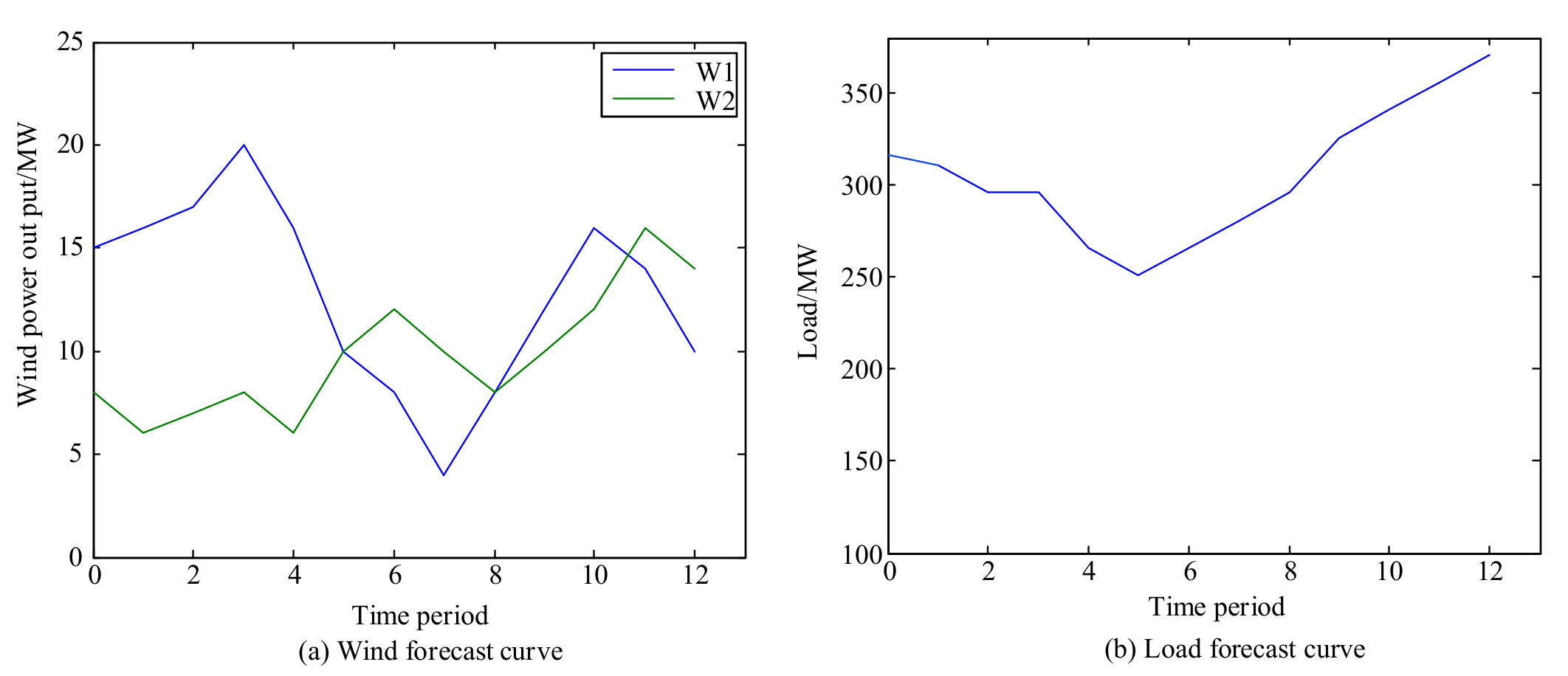
Conventional generator data used in IEEE 30-bus system are shown in

Table 1. Frequency regulation constant and cost coefficients of generators.

Generator No.	KG/p.u	Cost Coefficients
		ag	bg	cg
1	25.0	0.00375	2	0
2	20.0	0.0175	1.75	0
3	20.0	0.0625	1	0
4	20.0	0.00834	3.25	0
5	20.0	0.025	3	0
6	20.0	0.025	3	0

. Load and wind forecast value are shown in Figure 3. The forecast error of wind power is listed in

Table 2. Wind Forecast Error.

Time Period	Forecast Error	Time Period	Forecast Error
t1	5.13%	t7	11.43%
t2	6.26%	t8	12.25%
t3	7.54%	t9	13.17%
t4	8.67%	t10	13.86%
t5	9.21%	t11	14.39%
t6	10.37%	t12	15.78%

, which is obtained according to the historical data of wind power output in a province of China.

6.1. Dynamic Load Flow Results

To illustrate the difference between traditional power flow and DLF, the load flow results for IEEE 30-bus system at t₀ moment is shown in

Table 3. The real power output under dynamic load flow (DLF) and load flow (LF).

Generator No.	Set Value/MW	Power Output in DLF/MW	Power Output in LF/MW
1	180	184.41	188.04
2	57.56	58.69	57.56
3	24.56	25.27	24.56
4	35	35.49	35
5	17.93	18.35	17.93
6	16.91	17.48	16.91

and

Table 4. Line flow under DLF and LF.

Branch No.	Line Flow under DLF/MW	Line Flow under LF/MW	Branch No.	Line Flow under DLF/MW	Line Flow under LF/MW
1	123.61	120.93	22	8.91	8.93
2	64.43	63.48	23	5.61	5.63
3	39.46	39.14	24	−3.92	−3.9
4	60.15	59.26	25	6.18	6.16
5	65.93	65.32	26	−0.02	−0.06
6	50.9	50.41	27	36.66	36.67
7	50.19	49.48	28	21.27	21.28
8	−5.82	−5.69	29	18.57	18.58
9	29.04	28.9	30	9.43	9.46
10	0.65	0.21	31	−3.11	−3.1
11	30.9	30.54	32	6.11	6.15
12	21.06	20.94	33	−5.8	−5.75
13	−17.93	−18.35	34	3.55	3.55
14	48.83	48.9	35	−9.43	−9.38
15	40.42	39.95	36	22.89	22.85
16	−16.91	−17.48	37	6.21	6.21
17	9.45	9.46	38	7.12	7.12
18	23.89	23.94	39	3.71	3.71
19	12.79	12.84	40	5.45	5.5
20	3.12	3.13	41	17.56	17.46
21	9.11	9.15

.

It can be observed that the actual power output of generators and line flow obtained by DLF and LF is different. In traditional load flow, active power injection of all buses except slack bus are fixed. However, with the integration of renewable energy, the volatility of renewable energy can easily break the demand and generator balance. All generators with speed governor adjust their active power output according to their droop characteristic, which also impact the line flow.

Most references formulate their dispatch model based on traditional load flow, which cannot reflect the primary frequency regulation. Moreover, with the help of DLF, the primary and secondary frequency regulation amount can be easily quantified.

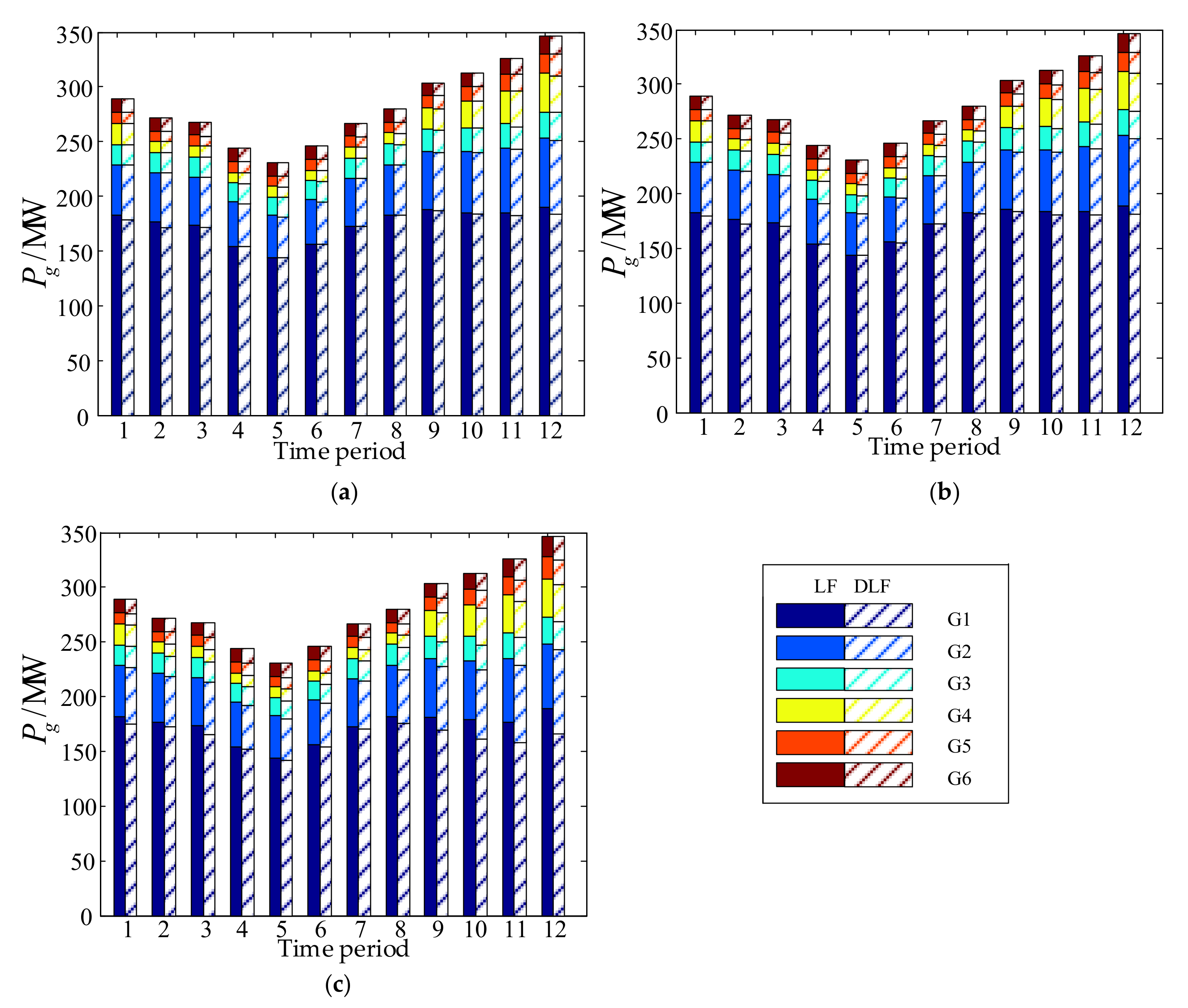
6.2. The Dispatch Results Comparison Based on LF and DLF

Figure 4 presents the dispatch results based on LF and DLF with different confidence levels of IEEE 30-bus system.

Table 5. Dispatch results comparison based on LF and DLF.

Confidence Level	DLF			LF
	Total Costs ($/h)	Primary Reserve		Total Costs ($/h)	Primary Reserve
		Up/MW	Down/MW		Up/MW	Down/MW
$1-\epsilon =0.8$	732.21	28.53	32.80	721.59	15.04	22.23
$1-\epsilon =0.9$	740.62	30.09	32.98	728.43	15.04	24.91
$1-\epsilon =1$	765.30	35.04	34.51	747.31	18.23	26.80

presents the total cost and the primary reserve of the dispatch results based on LF and DLF. The up/down primary reserve [7] is defined as:

$$\begin{array}{l}Upprimaryreserve=\min \left(\overline{P_g}-P_g,K_g\left(\overline{f}-f_N\right)\right)\\ Downprimaryreserve=\min \left(P_g-\underset{\_}{P_g},K_g\left(f_N-\underset{\_}{f}\right)\right)\end{array}$$

(42)

We can observe that the dispatch results based on LF and DLF is different. This is because, in the traditional dispatch model, once the nodal injection power fluctuates, only AGC units (in this paper, only the generator connected to the slack bus) adjust their power output to balance the generation and demand, and the primary regulation is neglected. Hence, the dispatch results based on LF and DLF is different.

On the other hand, from the dispatch results, since the traditional dispatch model doesn’t consider the regulation capability of non-AGC units, the low cost units will be dispatched first, and the high cost units will be dispatched last, which will lead to high cost units operate in lower limit and low cost units operate in upper limit, restraining the primary regulation capability. This is not beneficial for the frequency restoring when there is sharp increase or decrease of renewable energy. But in this paper, since the primary regulation of each generator is considered in DLF, the dispatch results can make sure the sufficiency of primary reserve to handle the volatility of renewable energy.

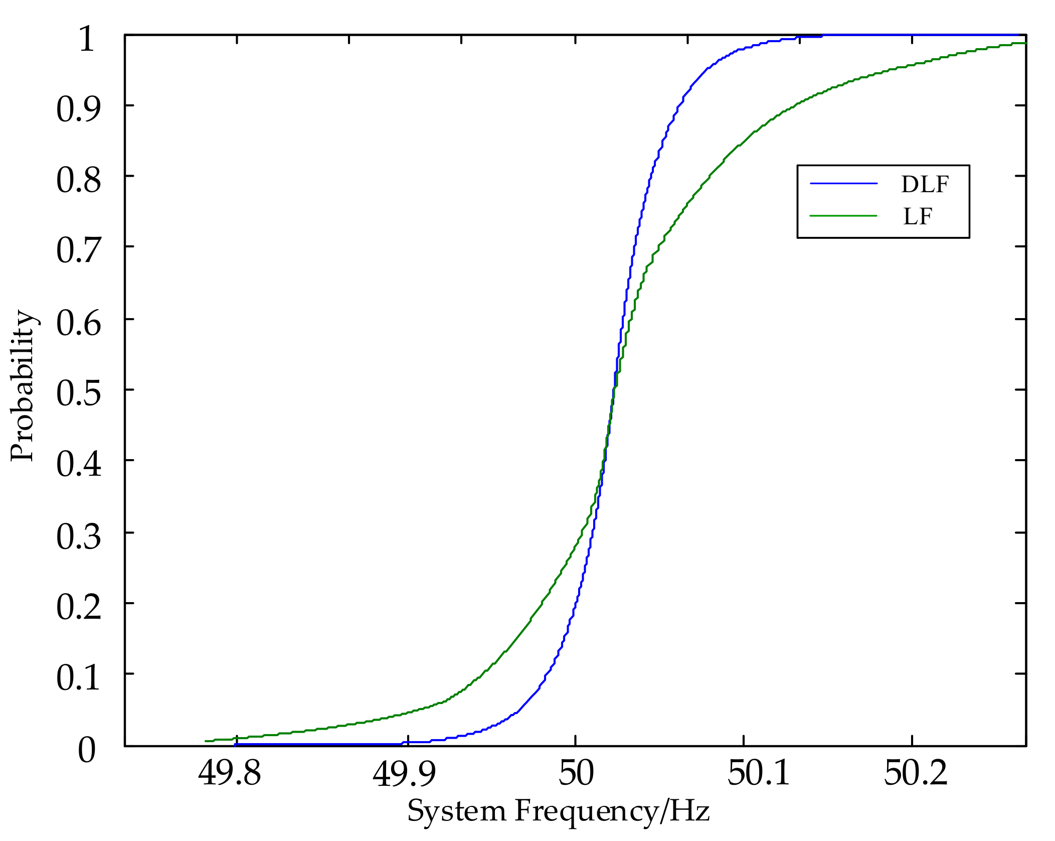
Although the operation cost of dispatch based on DLF is a little higher than that based on LF, the primary reserve of the former is more than the latter (shown in Table 5). Since renewable energy cannot keep to be its forecast value and it is easy to change, it is important to leave sufficient primary reserve to inhibit the fluctuation of system frequency. According to the dispatch results based on LF and DLF, one can obtain the frequency distribution based on both models. Figure 5 shows the CDF curve of frequency distribution at 12th time period. It is obvious that the variation of frequency based on DLF model is much smaller than that based on LF model. Moreover, it is possible for the dispatch results based on LF model that the frequency violates the allowed value (50 ± 0.2 Hz). Hence, the dispatch results based on DLF can immune the volatility of renewable energy better than that based on LF.

6.3. The Accuracy of CCP-CMCF

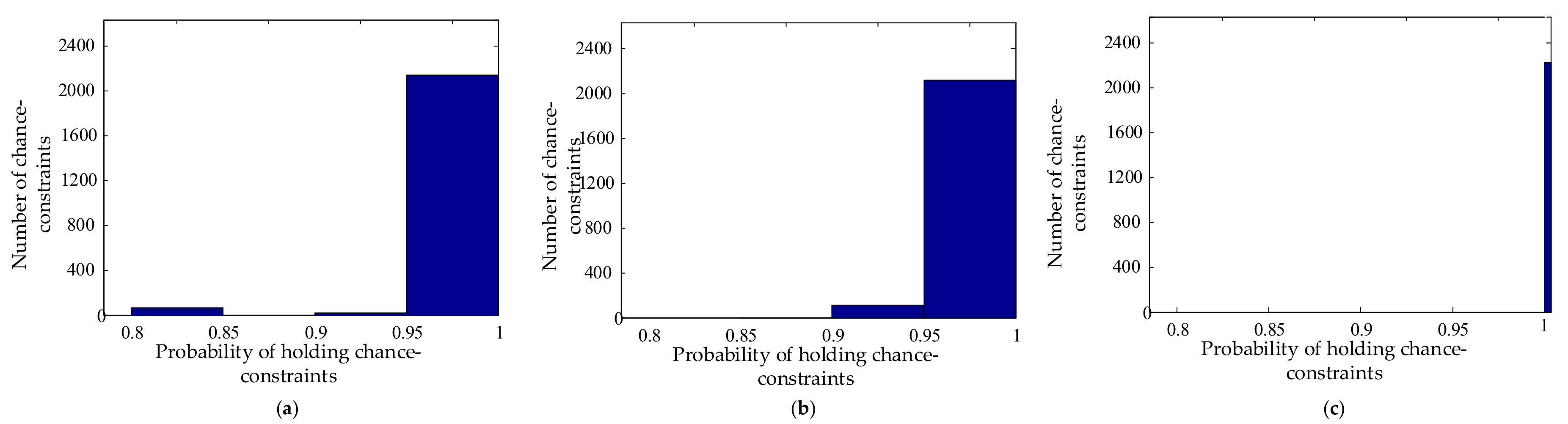
To demonstrate the accuracy of CCP-CMCF, a Monte-Carlo simulation is used to testify the obtained solution can satisfy all the chance constraints. According to the forecast value and forecast error of renewable energy in 6.1, 50,000 samples of each wind farm at each time period are randomly generated from the Laplace distribution. Regarding the spatial and temporal correlation, the normal transform and Cholesky decomposition described in [34] are adopted to transform the independent samples into correlated ones. For each sample, all the chance constraints are calculated using the obtained solution. Assuming that the number of samples that a constraint is respected is n, then the probability that this constraint is respected should be n/50,000 according to the large number theorem. By counting the constraints in each probability interval, Figure 6 can be obtained. It can be observed that the probability of holding the chance constraints are in accordance with the predetermined confidence interval, which verify that the dispatch results obtained through CCP-CMCF are accurate enough to handle the uncertainty of renewable energy.

6.4. The Influence of Confidence Level on the Dispatch Results

The confidence level also has an impact on the dispatch results. From Table 5 it can be observed that the total cost becomes higher with the increasing of confidence level. Specifically, when the confidence level is 1, this problem can be seen as a RO and the dispatch results can ensure the constraints are respected no matter how renewable energy fluctuates.

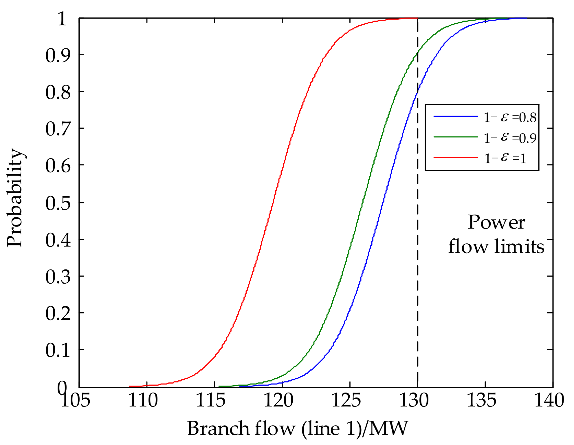
Based on the dispatch results, the power flow distribution of each time period can be obtained. The line flow distribution at 12th time period with different confidence levels of IEEE 30-bus system is shown in Figure 7. When the confidence level is less than 1, the violation of constraints is acceptable, but the probability of which is limited. When the confidence level is 1, the whole distribution curve is less than the line flow limit, but the cost is much higher. The operators of power system can make a trade-off between the total cost and the risk of violation.

6.5. The Influence of Correlation among Different Renewable Energy

The spatial correlation among different renewable energy sources and the temporal correlation among different time periods also have an impact on the dispatch results. Usually, the positive correlation will intensify the fluctuation of the total renewable outputs, which increases the total generation cost and vice versa. The simulation results presented in

Table 6. Dispatch results with or without correlation ($/h).

Confidence Level	With Correlation	Without Correlation
$1-\epsilon =0.8$	732.21	716.37
$1-\epsilon =0.9$	740.62	722.55
$1-\epsilon =1$	765.30	740.86

prove the assumption above.

6.6. Comparison between CCP-CMCF and Other CCP Methods

To demonstrate the advantages of the proposed CCP-CMCF, other two CCP methods are compared, i.e., CCP based on GMM (CCP-GMM) [23] and CCP based on analytical reformulation (CCP-AR) [22]. GMM is a powerful tool to fit various distributions, especially irregular distributions [23], but many Gaussian components may be needed to achieve desired accuracy, which will increase the computation burden to get the inverse of CDF. AR tries to reformulate the CDF by a simple function. It is easy to calculate the inverse of CDF, but it cannot make full use of the distribution properties, which may influence the accuracy of the dispatch results. The comparison among three methods is shown in

Table 7. Comparison among cumulants and cornish-fisher expansions (CMCF), gaussian mixture model (GMM) and analytical reformulation (AR) ($1-\epsilon =0.8$).

Test System	Computation Time (s)			Operation Cost ($/h)
	CMCF	GMM	AR	CMCF	GMM	AR
IEEE 30	0.89	5.02	1.13	732.21	747.23	756.52
IEEE 118	2.78	13.47	2.66	75,117.8	76,011.8	76,938.9
IEEE 300	11.78	38.59	13.82	430,827.6	439,233.7	456,292.1

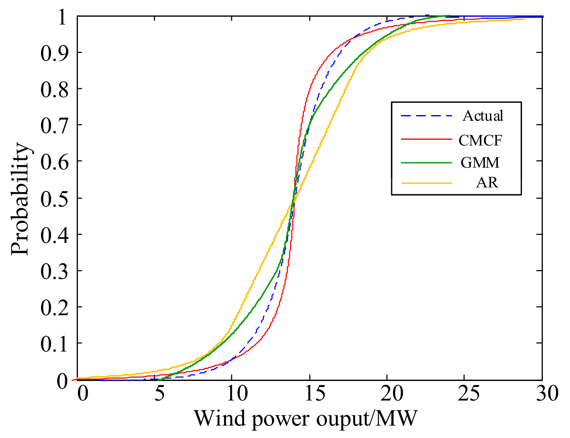
($1-\epsilon =0.8$). One can observe that CCP-CMCF has the lowest operation cost. This is because GMM and AR cannot accurately capture the tail properties of Laplace distribution and the inverse of CDF obtained by them are not accurate enough, leading to over-conservative results. Additionally, CMCF, GMM and AF are adopted to fit the wind power output distribution of wind farm 2 at 12th time period, as shown in Figure 8. It can be observed that the CDF curve of CMCF is much closer to the actual one compared with other two methods. Regarding the computation time, CCP-CMCF and CCP-AR are close, but CCP-GMM is much slower than the other two methods. Therefore, CCP-CMCF is proved to be efficient to solve the real-time dispatch problem.

7. Conclusions

In this paper, we propose a real-time dispatch with renewable uncertainty based on DLF, in which the frequency constraint and the regular constraints like generator production limits, line flow limits are respected under both primary and secondary frequency regulation.

To solve the dispatch problem with renewable uncertainty, CCP-CMCF is adopted in which cumulants and Cornish-fisher expansions are adopted to get the probability of holding the chance constraints and then the real-time dispatch model can be transformed into a quadratic programming.

The simulation results show that the dispatch results based on DLF are different from the traditional ones based on LF. The former can ensure the dispatch results have sufficient primary reserve to immunize against the volatility of renewable energy and restrain the fluctuation of system frequency. The proposed CCP-CMCF also has high computational speed without sacrificing the accuracy of the results. The confidence level, spatial and temporal correlation of renewable sources also influence the dispatch results. If the correlation is neglected, great errors may arise. Besides, the operators of a power system can choose an appropriate confidence level to balance the economy and the security of their system.

References

1. Lee, T.Y. Optimal Spinning Reserve for a Wind-Thermal Power System Using EIPSO. IEEE Trans. Power Syst. 2007, 22, 1612–1621. [Google Scholar] [CrossRef]
2. Li, Z.; Wu, W.; Zhang, B.; Wang, B. Adjustable Robust Real-Time Power Dispatch with Large-Scale Wind Power Integration. IEEE Trans. Sustain. Energy 2015, 6, 357–368. [Google Scholar] [CrossRef]
3. Jabr, R.A. Adjustable Robust OPF with Renewable Energy Sources. IEEE Trans. Power Syst. 2013, 28, 4742–4751. [Google Scholar] [CrossRef]
4. Lee, Y.Y.; Baldick, R. A frequency-constrained stochastic economic dispatch model. IEEE Trans. Power Syst. 2013, 28, 2301–2312. [Google Scholar] [CrossRef]
5. Li, N.; Zhao, C.; Chen, L. Connecting Automatic Generation Control and Economic Dispatch from an Optimization View. IEEE Trans. Control Netw. Syst. 2016, 3, 254–264. [Google Scholar] [CrossRef]
6. Cai, D.; Mallada, E.; Wierman, A. Distributed optimization decomposition for joint economic dispatch and frequency regulation. IEEE Trans. Power Syst. 2017, 32, 4371–4385. [Google Scholar] [CrossRef]
7. Restrepo, J.F.; Galiana, F.D. Unit commitment with primary frequency regulation constraints. IEEE Trans. Power Syst. 2005, 20, 1836–1842. [Google Scholar] [CrossRef]
8. Eto, J.H.; Undrill, J.; Mackin, P.; Daschmans, R.; Williams, B.; Haney, B.; Hunt, R.; Ellis, J.; Illian, H.F.; Martinez, C.; et al. Use of Frequency Response Metrics to Assess the Planning and Operating Requirements for Reliable Integration of Variable Renewable Generation; Lawrence Berkeley National Laboratory: Berkeley, CA, USA, 2011. [Google Scholar]
9. Ramanathan, R.; Ramchandani, H.; Sackett, S.A. Dynamic Load Flow Technique for Power System Simulators. IEEE Trans. Power Syst. 1986, 1, 25–30. [Google Scholar] [CrossRef]
10. Roytelman, I.; Shahidehpour, S.M. A comprehensive long term dynamic simulation for power system recovery. IEEE Trans. Power Syst. 1994, 9, 1427–1433. [Google Scholar] [CrossRef]
11. Okamura, M.; O-ura, Y.; Hayashi, S.; Uemura, K. A new power flow model and solution method including load and generator characteristics and effects of system control devices. IEEE Trans. Power Appar. Syst. 1975, 94, 1042–1050. [Google Scholar] [CrossRef]
12. Duan, Y.; Zhang, B. An improved fast decoupled power flow model considering static power–frequency characteristic of power systems with large-scale wind power. IEEE J. Trans. Electr. Electron. Eng. 2014, 9, 151–157. [Google Scholar] [CrossRef]
13. Lorca, Á.; Sun, X.A. Adaptive Robust Optimization with Dynamic Uncertainty Sets for Multi-Period Economic Dispatch under Significant Wind. IEEE Trans. Power Syst. 2015, 30, 1702–1713. [Google Scholar] [CrossRef]
14. Wu, W.; Chen, J.; Zhang, B.; Sun, H. A Robust Wind Power Optimization Method for Look-Ahead Power Dispatch. IEEE Trans. Sustain. Energy 2014, 5, 507–515. [Google Scholar] [CrossRef]
15. Xie, L.; Gu, Y.; Zhu, X.; Genton, M.G. Short-Term Spatio-Temporal Wind Power Forecast in Robust Look-ahead Power System Dispatch. IEEE Trans. Smart Grid 2014, 5, 511–520. [Google Scholar] [CrossRef]
16. Lu, Z.G.; Zhao, H.; Xiao, H.F.; Zhang, J.F.; Li, X.P.; Sun, X.F. Robust DED based on bad scenario set considering wind, EV and battery switching station. IET Gener. Transm. Distrib. 2017, 11, 354–362. [Google Scholar]
17. Xiong, P.; Jirutitijaroen, P. Two-Stage adjustable robust optimisation for unit commitment under uncertainty. IET Gener. Transm. Distrib. 2014, 8, 573–582. [Google Scholar] [CrossRef]
18. Liu, Y.; Nair, N.C. A Two-Stage Stochastic Dynamic Economic Dispatch Model Considering Wind Uncertainty. IEEE Trans. Sustain. Energy 2016, 7, 819–829. [Google Scholar] [CrossRef]
19. Gangammanavar, H.; Sen, S.; Zavala, V.M. Stochastic Optimization of Sub-Hourly Economic Dispatch with Wind Energy. IEEE Trans. Power Syst. 2016, 31, 949–959. [Google Scholar] [CrossRef]
20. Zhang, H.; Li, P. Chance Constrained Programming for Optimal Power Flow under Uncertainty. IEEE Trans. Power Syst. 2011, 26, 2417–2424. [Google Scholar] [CrossRef]
21. Vrakopoulou, M.; Margellos, K.; Lygeros, J.; Andersson, G. A Probabilistic Framework for Reserve Scheduling and Security Assessment of Systems with High Wind Power Penetration. IEEE Trans. Power Syst. 2013, 28, 3885–3896. [Google Scholar] [CrossRef]
22. Roald, L.; Oldewurtel, F.; Parys, B.V.; Andersson, G. Security Constrained Optimal Power Flow with Distributionally Robust Chance Constraints. arXiv, 2015; arXiv:1508.06061. [Google Scholar]
23. Hu, Y.; Li, Y.; Xu, M.; Zhou, L.; Cui, M. A chance-constrained economic dispatch model in wind-thermal-energy storage system. Energies 2017, 10, 326. [Google Scholar] [CrossRef]
24. Glover, J.D.; Sarma, M.S.; Overbye, T.J. Power System Analysis & Design, 5th ed.; Cengage Learning: Stamford, CT, USA, 2012; pp. 657–662. [Google Scholar]
25. Charnes, A.; Cooper, W.W. Chance-constrained programming. Manag. Sci. 1959, 6, 73–79. [Google Scholar] [CrossRef]
26. Liu, J.; Hao, X.; Cheng, P.; Fang, W.; Niu, S. A parallel probabilistic load flow method considering nodal correlations. Energies 2016, 9, 1041. [Google Scholar] [CrossRef]
27. Fan, M.; Vittal, V.; Heydt, G.T.; Ayyanar, R. Probabilistic power flow studies for transmission systems with photovoltaic generation using cumulants. IEEE Trans. Power Syst. 2012, 27, 2251–2261. [Google Scholar] [CrossRef]
28. Usaola, J. Probabilistic load flow in systems with wind generation. IET Gener. Transm. Distrib. 2009, 3, 1031–1041. [Google Scholar] [CrossRef] [Green Version]
29. Wu, W.; Wang, K.; Li, G.; Jiang, X.; Wang, Z. Probabilistic load flow calculation using cumulants and multiple integrals. IET Gener. Transm. Distrib. 2016, 10, 1703–1709. [Google Scholar] [CrossRef]
30. Deng, X.; He, J.; Zhang, P. A Novel Probabilistic Optimal Power Flow Method to Handle Large Fluctuations of Stochastic Variables. Energies 2017, 10, 1623. [Google Scholar] [CrossRef]
31. Morales, J.M.; Baringo, L.; Conejo, A.J. Probabilistic power flow with correlated wind sources. IET Gener. Transm. Distrib. 2010, 4, 641–651. [Google Scholar] [CrossRef]
32. Fisher, S.R.A.; Cornish, E.A. The percentile points of distributions having known cumulants. Technometrics 1960, 2, 209–225. [Google Scholar] [CrossRef]
33. Wu, J.; Zhang, B.; Li, H.; Li, Z.; Chen, Y.; Miao, X. Statistical distribution for wind power forecast error and its application to determine optimal size of energy storage system. Int. J. Electr. Power Energy Syst. 2014, 55, 100–107. [Google Scholar] [CrossRef]
34. Cai, D.; Shi, D.; Chen, J. Probabilistic load flow computation with polynomial normal transformation and Latin hypercube sampling. IET Gener. Transm. Distrib. 2013, 7, 474–482. [Google Scholar] [CrossRef]
Figure 1. Power-frequency relation of generators and load.
Energies 10 02111 g001
Figure 2. Flowchart of chance-constrained programming based on cumulants and Cornish-fisher expansions (CCP-CMCF).
Energies 10 02111 g002
Figure 3. (a) Wind forecast curve; (b) Load forecast curve.
Energies 10 02111 g003
Figure 4. Dispatch results of generators in IEEE 30-bus system with different confidence levels. (a) 1 ε = 0.8 ; (b) 1 ε = 0.9 ; (c) 1 ε = 1 .
Energies 10 02111 g004
Figure 5. Frequency distribution based on DLF and LF.
Energies 10 02111 g005
Figure 6. Probability histogram of chance constraints in IEEE 30-bus system with different confidence levels. (a) 1 ε = 0.8 ; (b) 1 ε = 0.9 ; (c) 1 ε = 1 .
Energies 10 02111 g006
Figure 7. Line flow distribution under different confidence level.
Energies 10 02111 g007
Figure 8. Wind power output distribution of wind farm 2.
Energies 10 02111 g008