The General Regression Neural Network Based on the Fruit Fly Optimization Algorithm and the Data Inconsistency Rate for Transmission Line Icing Prediction


Abstract
:1. Introduction
2. Methodology
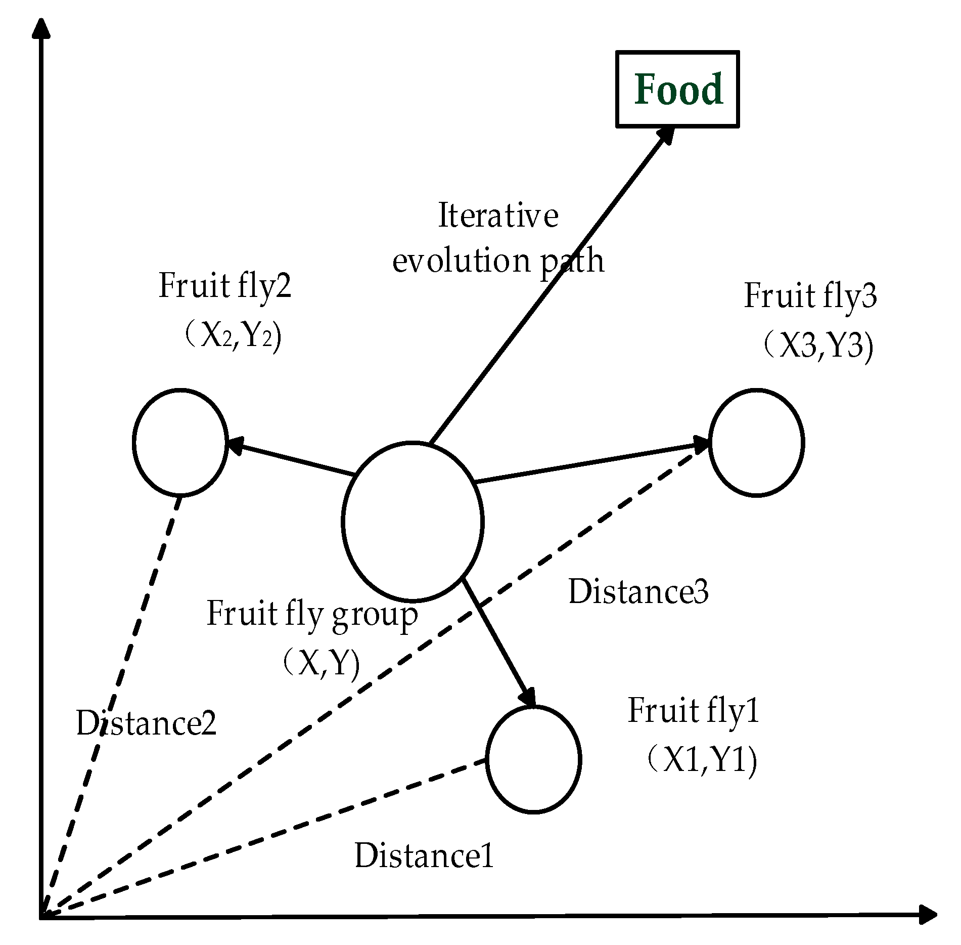
2.1. Fruit Fly Optimization Algorithm
- (1)
- Initialize the population size Sizepop, the iterations Maxgen, and the position coordinates (X0, Y0) of the random fruit fly population.
- (2)
- Give the individual fruit flies’ random flight direction and step size so that they can find food by using the smell:Where
- (3)
- Since the fruit flies cannot obtain the food position, the distance Disti between the individual and the origin of the flies is estimated first, and the taste concentration determination value Si is calculated:
- (4)
- Put the taste concentration determination value Si into the adaptation function Fitness to determine the taste concentration Smelli of the individual position.
- (5)
- Identify the individual of the highest concentration among the fruit fly populations including the concentration and coordinates:
- (6)
- Retain the maximum taste concentration value best Smell and its individual coordinates. The fruit fly population uses vision to fly in that direction:
2.2. Data Inconsistency Rate
- (1)
- Initialize the optimal feature subset as null set .
- (2)
- Calculate the inconsistent rate of the data sets G1, G2, ..., Gg in the feature subsets which are made up with the remaining feature of each subset.
- (3)
- Select the feature Gi which corresponds to the minimum inconsistent rate as the optimum feature, and then update the optimum feature subset to .
- (4)
- Calculate the inconsistent rate statistics table of the feature subsets and arrange them from small to large.
- (5)
- Select the feature subsets with the smallest number of features, which can be selected as the optimal feature subsets if they satisfy the condition that or is the minimum of the inconsistent rate of all adjacent feature subsets. is an adjacent feature subset of .
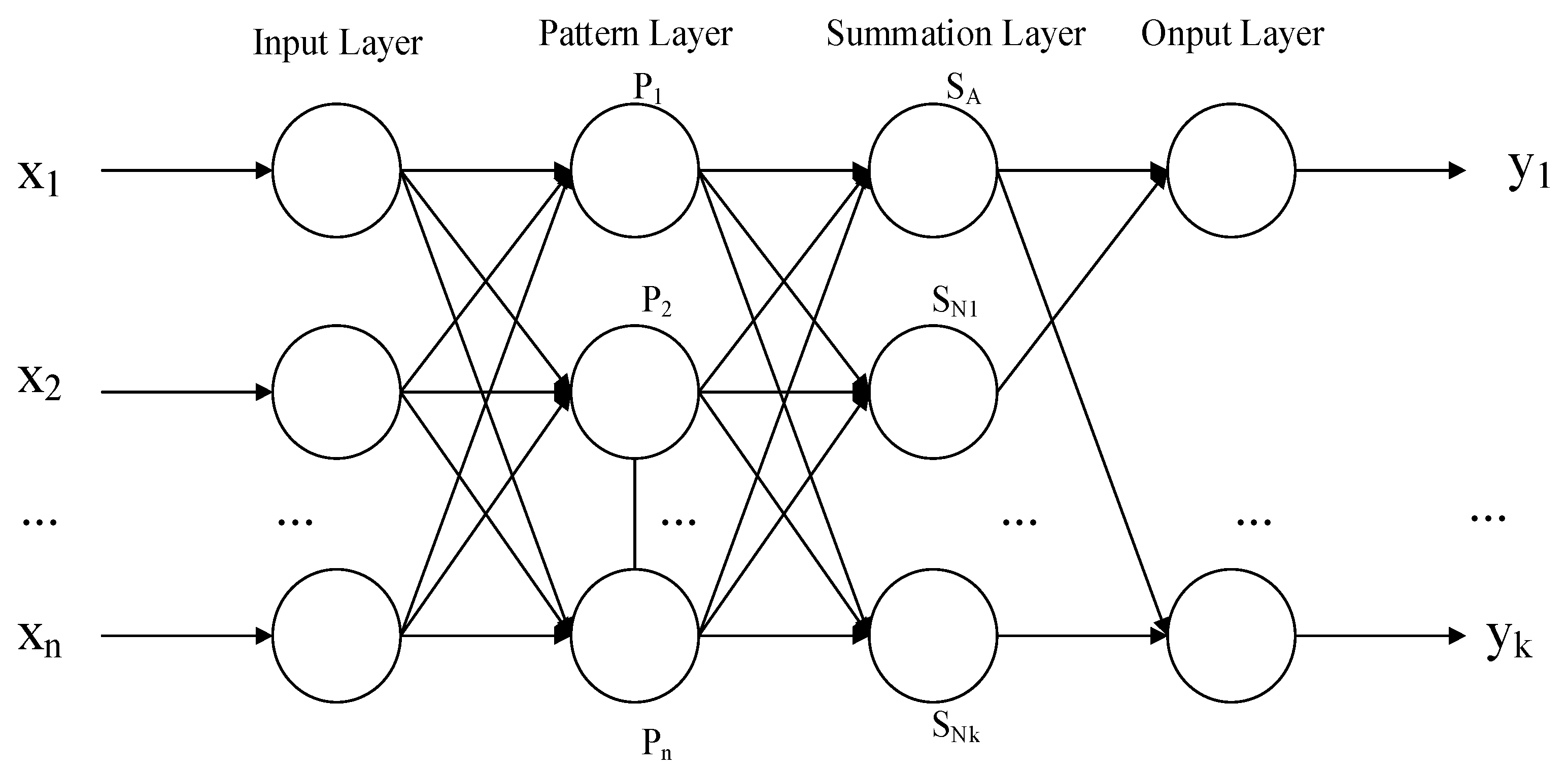
2.3. Generalized Regression Neural Network
- (1)
- The input layer: the original variables enter the network which correspond to the neurons one by one and are submitted to the next layer.
- (2)
- The pattern layer: nonlinear transformation is applied to the values received from the input layer. The transfer function of the ith neuron in the pattern layer is:where X represents input variable, Xi is the learning sample corresponding to the ith neuron; and is the smoothing parameter.
- (3)
- The summation layer: calculate the sum and weighted sum of the pattern outputs.The summation layer contains two types of neurons, in which one neuron SA makes arithmetic summation of the output of all pattern layer neurons, and the connection weight of each neuron in the pattern layer to this neuron is 1. Its transfer function is:The outputs of all neurons in the pattern layer were weighted and summed to gain the other neurons SNj in the summation layer. The transfer function of the other neurons in the summation layer is:where yij is the connection weight between the ith neuron in the pattern layer and the jth neuron in the summation layer. yij is the jth element in the ith output sample yi.
- (4)
- The output layer: the forecasting results can be derived. The output of each neuron is:where yj is the output of the jth neuron.
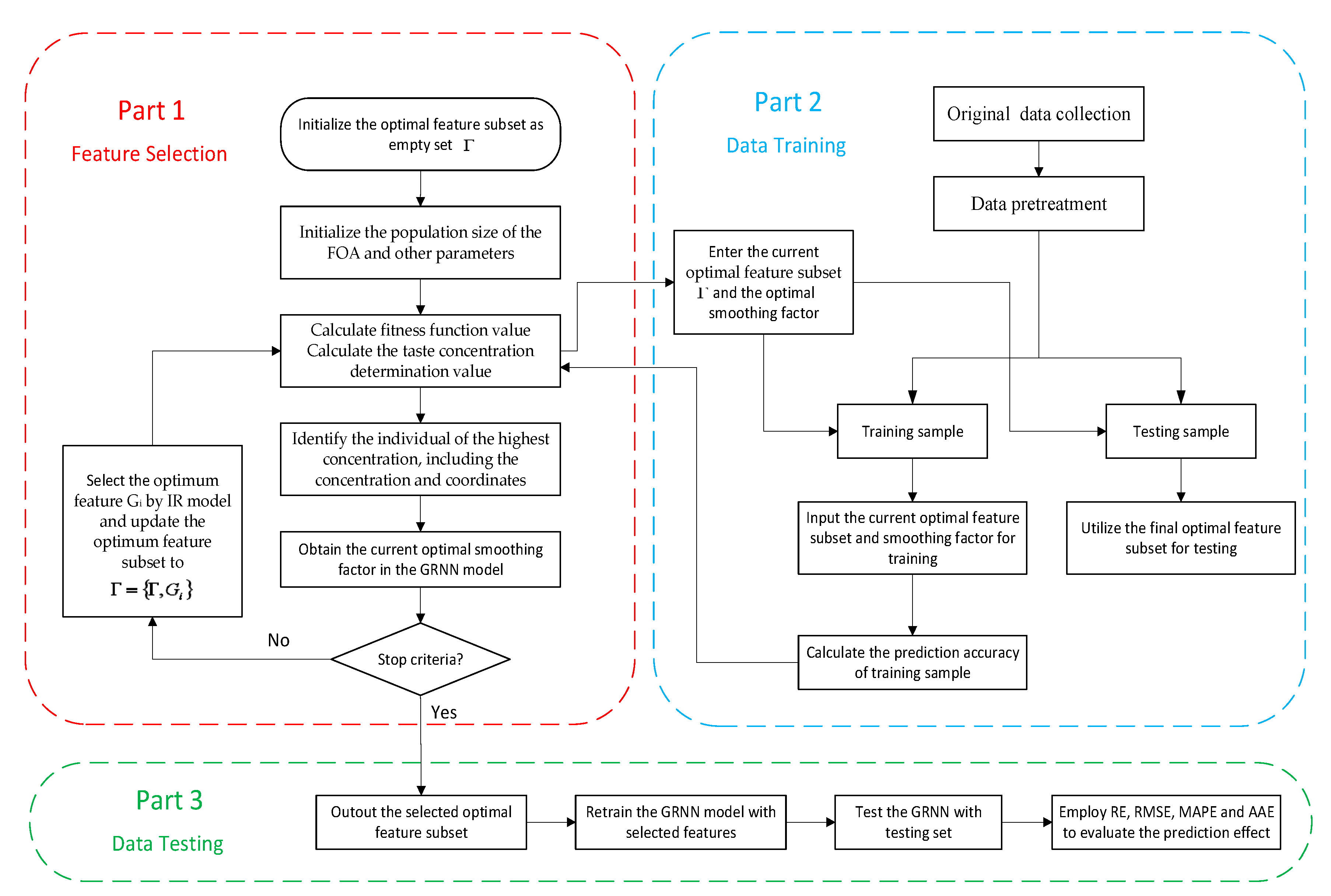
2.4. The Forecasting Model of FOA-IR-GRNN
- (1)
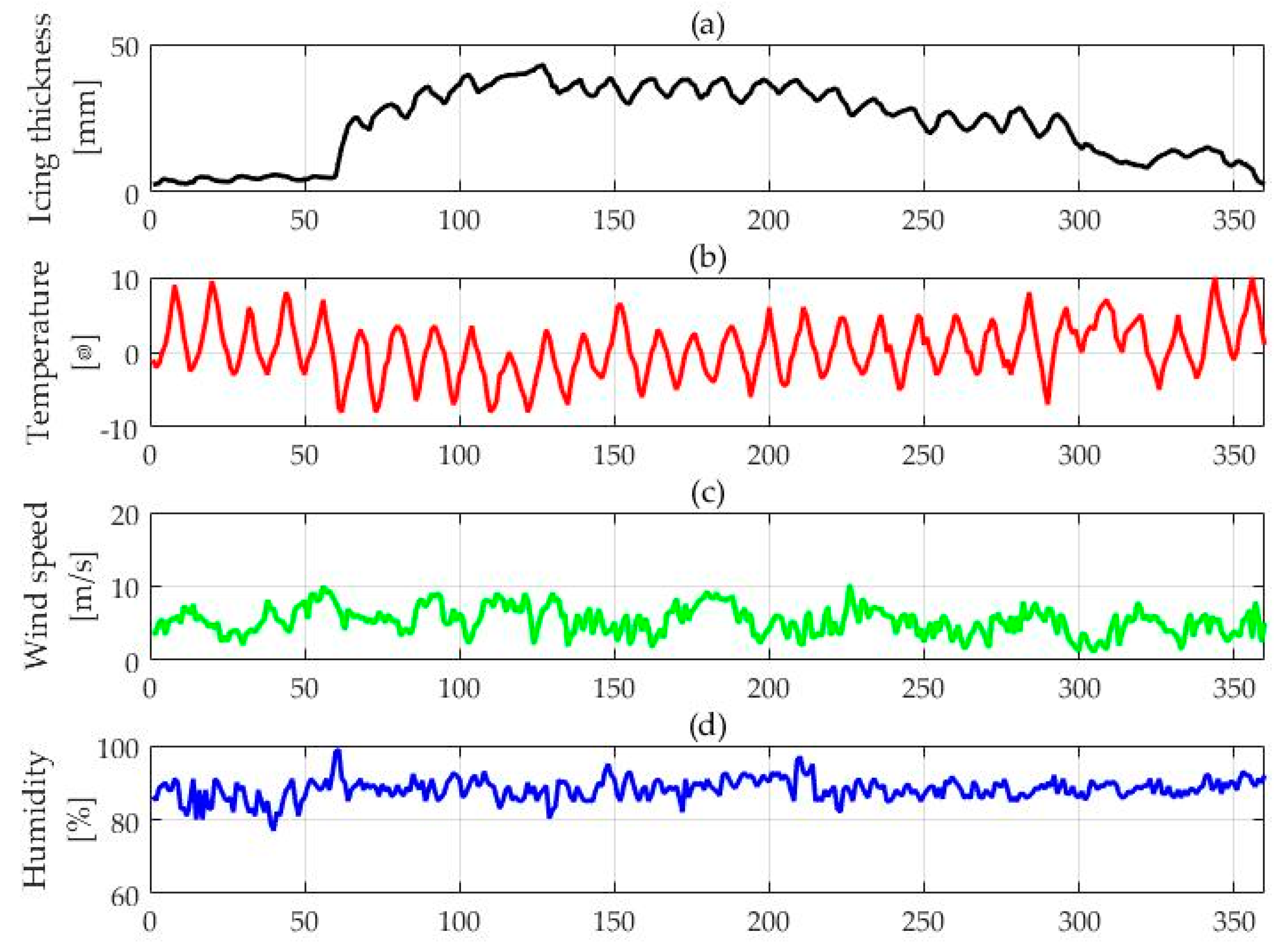
- Determine the initial candidate feature. In this paper, we choose ambient temperature, relative humidity, wind speed, wind direction, light intensity, atmospheric pressure, altitude, condensation height, conductor direction, the height of conductor suspension, load current, precipitation, and conductor surface temperature, all of which are selected as the candidate features of the factors that influence icing. In addition, when it reaches the point t-i (i = 1, 2, 3, 4), thickness value, temperature, relative humidity and wind speed are also selected as the main influencing factors of line icing. All the initial candidate features are shown in Table 1. In the IR algorithm, the optimal feature subset needs to be initialized as an empty set .
- (2)
- Initialize the parameters of FOA. Suppose the population size is 20, the maximum iteration number is 200 and the range of random flight distance is set as [−10, 10].
- (3)
- Calculate the inconsistent rate. After completing steps (1) and (2), put the candidate features into the IR feature selection model gradually. Calculate the inconsistent rate of the data sets G1, G2, …, Gg in the feature subsets which are made up of the remaining features of each subset and then select the feature Gi which corresponds to the minimum inconsistent rate as the optimum feature, and update the optimum feature as .
- (4)
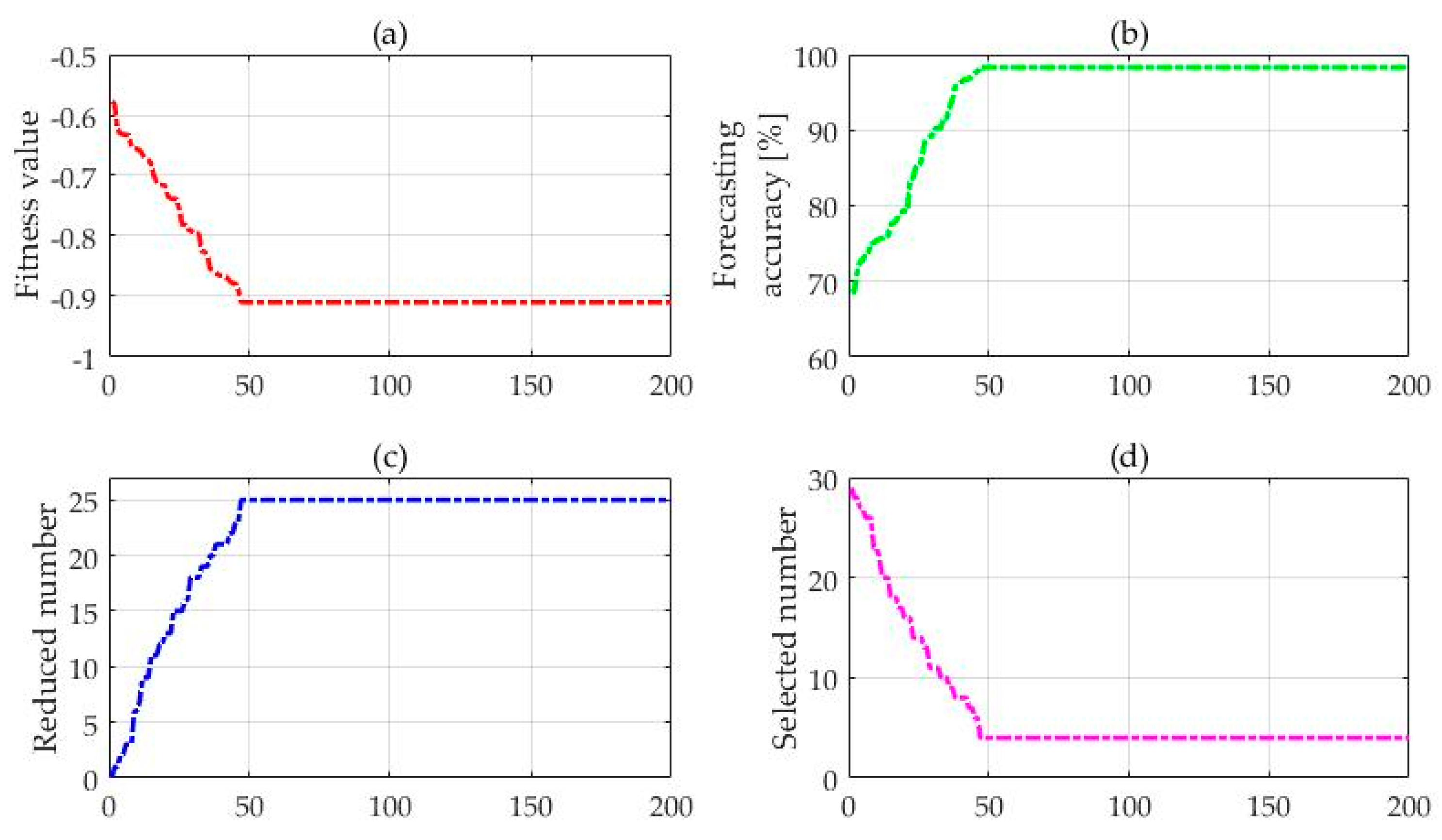
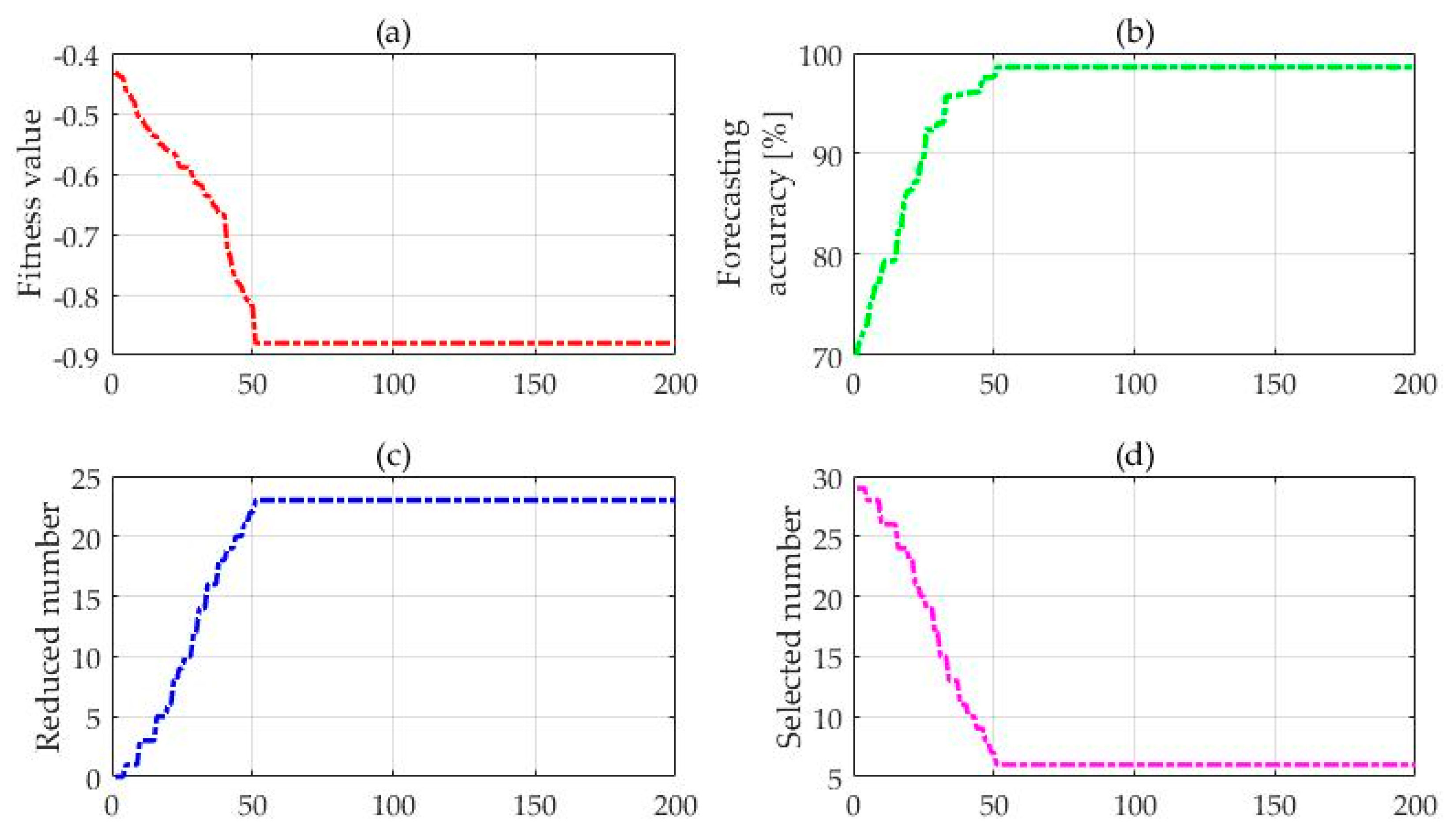
- Get the optimal feature subset and the best value of smoothing factor in GRNN. Put the current feature subsets into the GRNN model, and calculate the prediction accuracy during the learning process of the circular training samples. Then, the fitness function Fitness(j) can be worked out. We can get the optimum feature subset by comparing the fitness function among each generation and judge whether all iterations have achieved the algorithm stopping conditions. If not, re-initialize a new feature subset and put it into a new circulation until the optimum feature subset which meets all the conditions is obtained. It should be noted that the smoothing factor of the GRNN also needs to be optimized, and the initial value of smoothing factor will be assigned randomly. In this paper, a fitness function is established based on the two factors of prediction accuracy and feature selection:In the formula, Numfeature(xi) is the number of optimum feature which is selected by each iteration and both a and b are constants between [0, 1]; r(j) represents the prediction accuracy of ice cover thickness at each iteration. The optimal number of features is proportional to the fitness function for all iterations, and the accuracy of the icing prediction is inversely proportional to the fitness function. Different smoothing factors will result in different forecasting results and lead to different prediction accuracy, indicating that the smoothing factor of the GRNN also influences the value of fitness function Fitness(j). Hence the optimal feature subset and the best value of smoothing factor in the GRNN will be obtained at the same time in this step.
- (5)
- Stop optimization and start prediction. Circulation ends at the maximum number of iteration. Here, the optimum feature subset and the best value of smoothing factor can be substituted into the GRNN model for icing thickness forecasting.
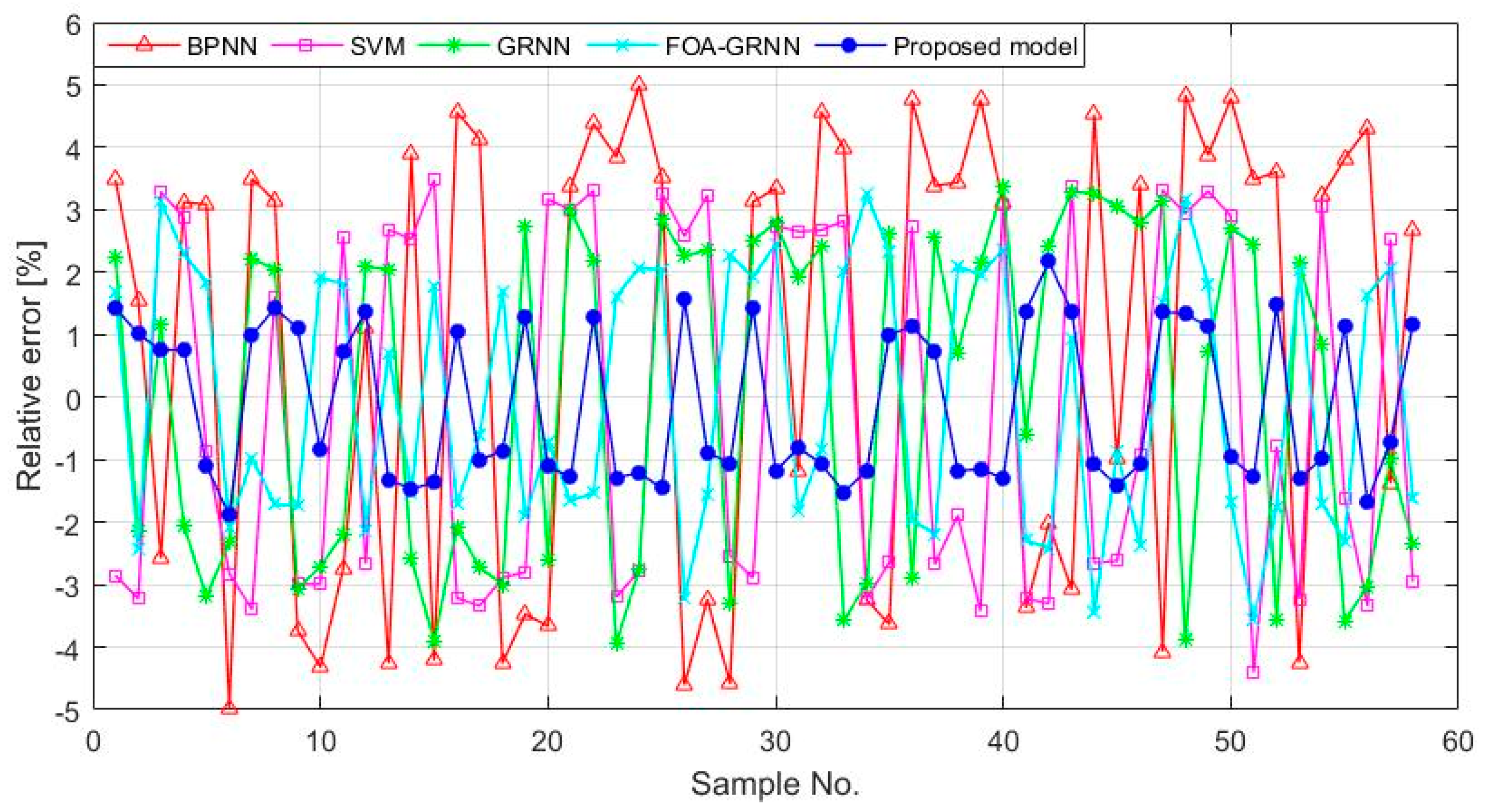
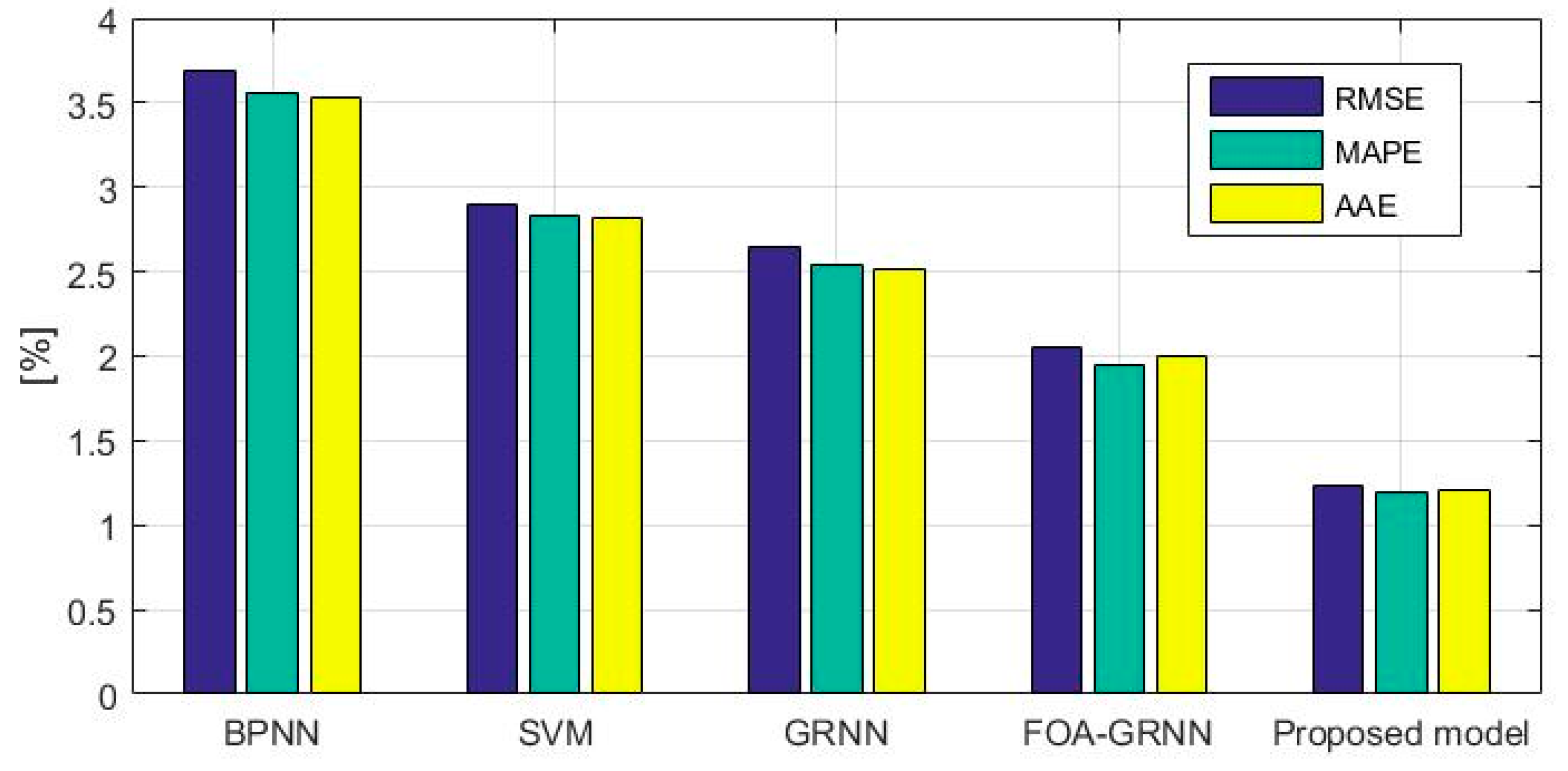
3. Performance Evaluation Index
4. Empirical Analysis
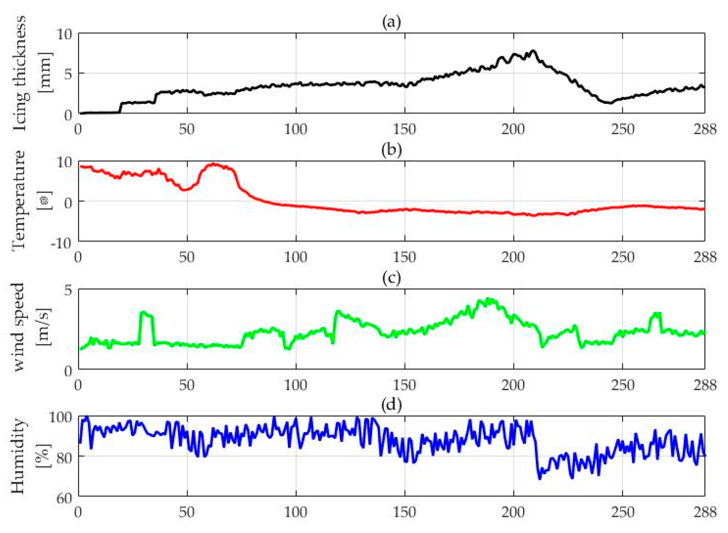
4.1. Data Collection and Pretreatment
4.2. Feature Selection
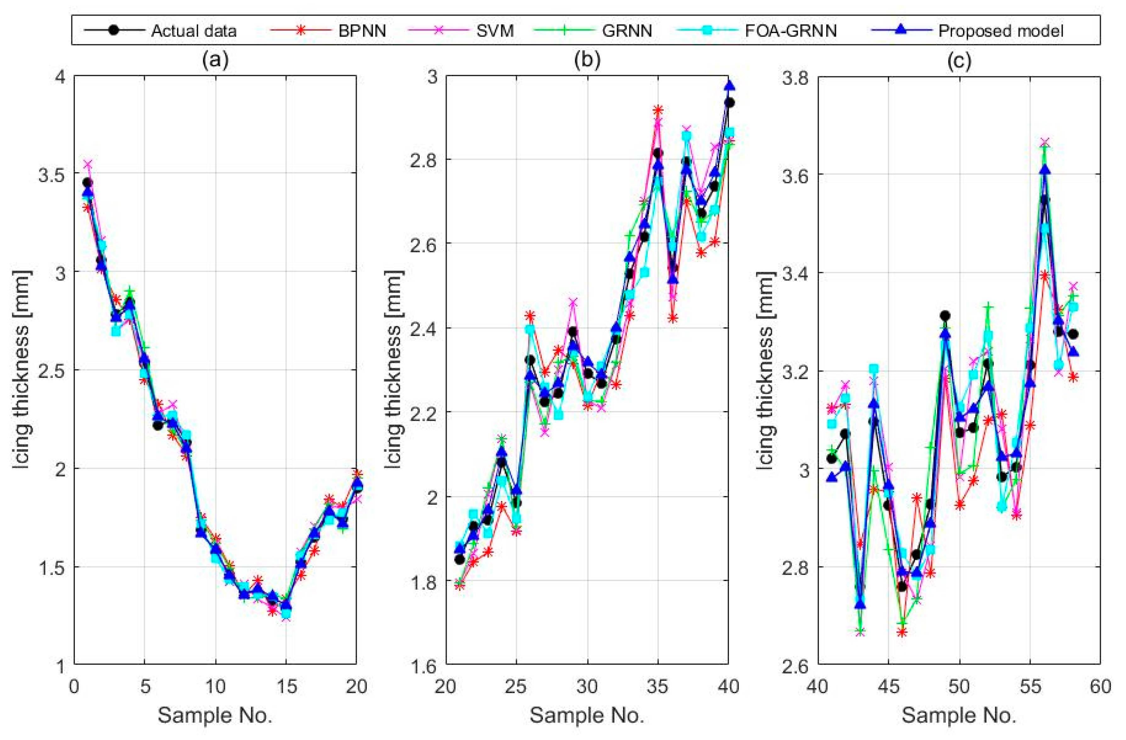
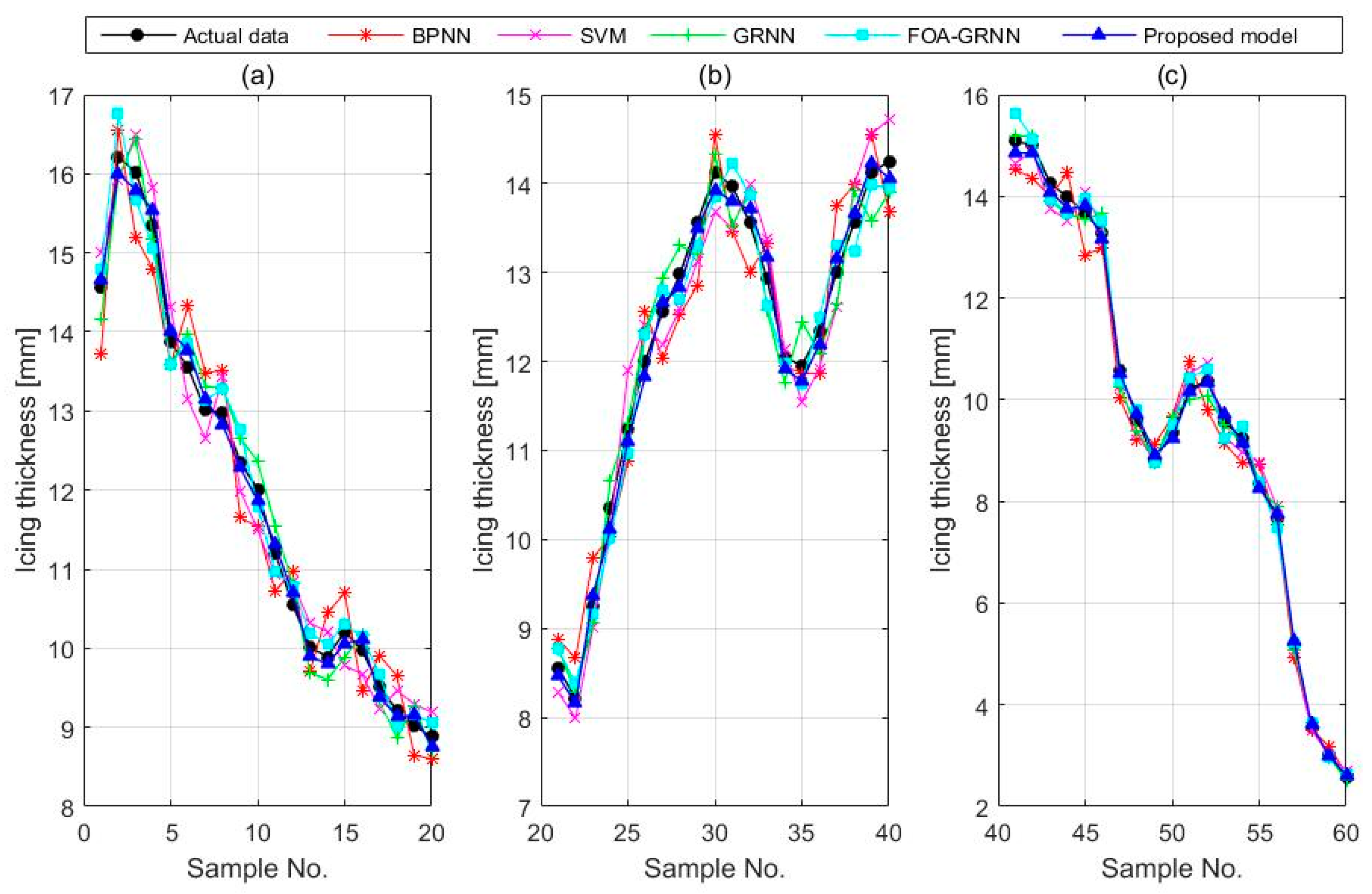
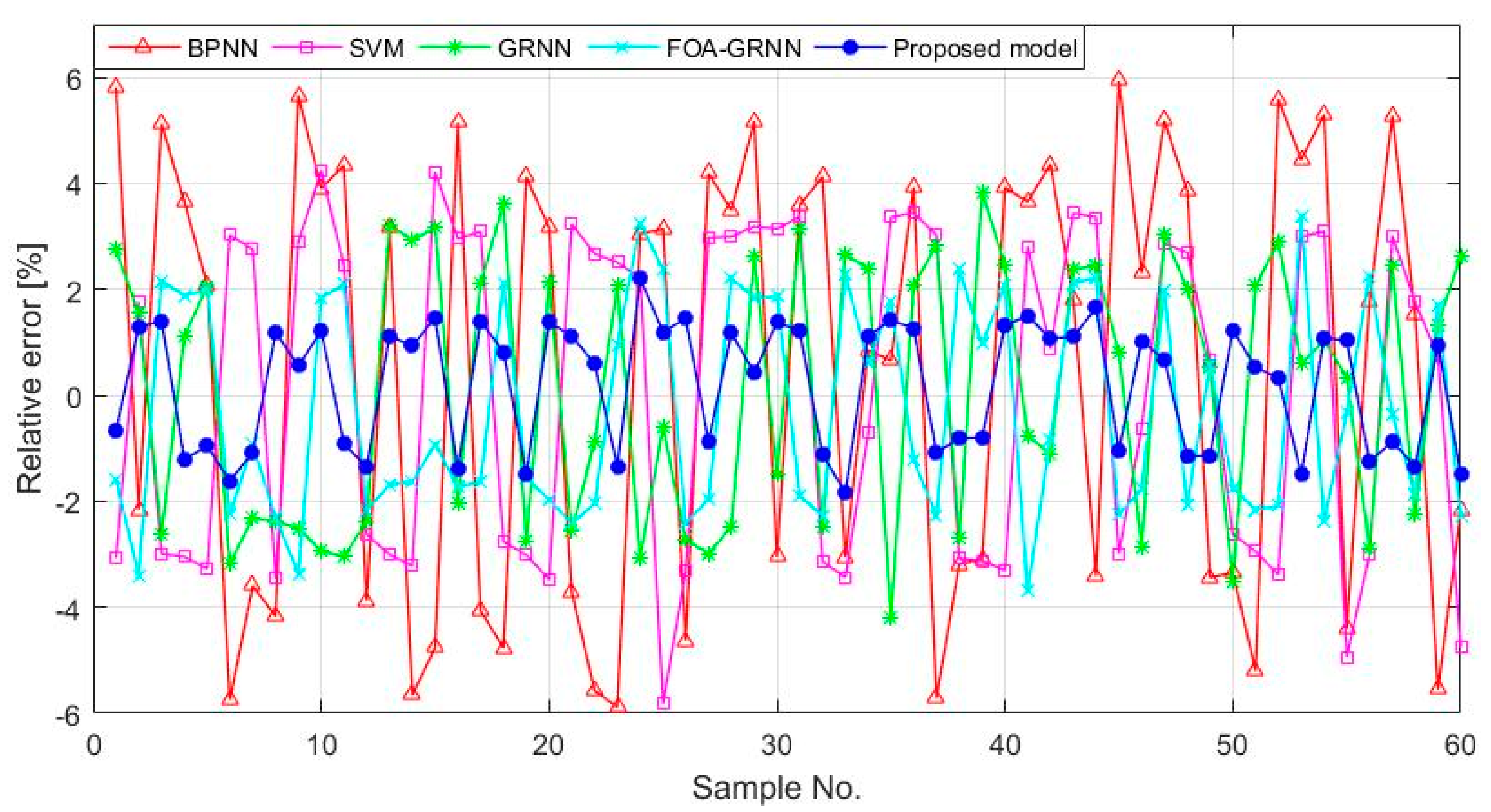
4.3. The GRNN for Icing Forecasting
5. Case Study 2
6. Conclusions
Acknowledgments
Author Contributions
Conflicts of Interest
References
- Tian, H.; Liang, N.; Zhao, P.; Wang, X.; Zhu, C.; Zhang, S.; Wang, W. Model updating approach for icing forecast of transmission lines by using particle swarm optimization. IOPscience 2017, 207. [Google Scholar] [CrossRef]
- Lamraoui, F.; Fortin, G.; Benoit, R.; Perron, J.; Masson, C. Atmospheric icing severity: Quantification and mapping. Atmos. Res. 2013, 128, 57–75. [Google Scholar] [CrossRef]
- Zhang, W.L.; Yu, Y.Q.; Su, Z.Y.; Fan, J.B.; Li, P.; Yuan, D.L.; Wu, S.Y.; Song, G.; Deng, Z.F.; Zhao, D.L.; et al. Investigation and analysis of icing and snowing disaster happened in hunan power grid in 2008. Power Syst. Technol. 2008, 32, 1–5. [Google Scholar]
- Zhuang, W.; Zhang, H.; Zhao, H.; Wu, S.; Wan, M. Review of the Research for Power line Icing Prediction. Adv. Meteorol. Sci. Technol. 2017, 7, 6–12. [Google Scholar]
- Liang, X.; Li, Y.; Zhang, Y.; Liu, Y. Time-dependent simulation model of ice accretion on transmission line. High Volt. Eng. 2014, 40, 336–343. [Google Scholar]
- Liu, C.C.; Liu, J. Ice accretion mechanism and glaze loads model on wires of power transmission lines. High Volt. Eng. 2011, 37, 241–248. [Google Scholar]
- Imai, I. Studies on ice accretion. Res. Snow Ice 1953, 3, 35–44. [Google Scholar]
- Goodwin, E.J.I.; Mozer, J.D.; Digioia, A.M.J.; Power, B.A. Predicting Ice and Snow Loads for Transmission Line Design. Available online: http://www.dtic.mil/docs/citations/ADP001696 (accessed on 11 August 2017).
- Lenhand, R.W. An indirect method for estimating the weight of glaze on wires. Bull. Am. Meteorol. Soc. 1995, 36, 1–5. [Google Scholar]
- Huang, X.B.; Li, H.B.; Zhu, Y.C.; Wang, Y.X.; Zheng, X.X.; Wang, Y.G. Transmission line icing short-term forecasting based on improved time series analysis by fireworks algorithm. In Proceedings of the International Conference on Condition Monitoring and Diagnosis, Xi’an, China, 25–28 September 2016. [Google Scholar]
- Yang, J.L. Impact on the Extreme Value of Ice Thickness of Conductors from Probability Distribution Models. In Proceedings of the International Conference on Mechanical Engineering and Control Systems, Wuhan, China, 23–25 January 2015. [Google Scholar]
- Liu, C.; Liu, H.W.; Wang, Y.S.; Lu, J.Z.; Xu, X.J.; Tan, Y.J. Research of icing thickness on transmission lines based on fuzzy Markov chain prediction. In Proceedings of the IEEE International Conference on Applied Superconductivity and Electromagnetic Devices (ASEMD), Beijing, China, 25–27 October 2013. [Google Scholar]
- Chen, S.; Dong, D.; Huang, X.; Sun, M. Short-Term Prediction for Transmission Lines Icing Based on BP Neural Network. In Proceedings of the Asia-Pacific Power and Energy Engineering Conference, Shanghai, China, 27–29 March 2012. [Google Scholar]
- Ma, T.; Niu, D.; Fu, M. Icing Forecasting for Power Transmission Lines Based on a Wavelet Support Vector Machine Optimized by a Quantum Fireworks Algorithm. Appl. Sci. 2016, 6, 54. [Google Scholar] [CrossRef]
- Luo, Y.; Yao, Y.; Ying, L.I.; Wang, K.; Qiu, L. Study on Transmission Line Ice Accretion Mode Based on BP Neural Network. J. Sichuan Univ. Sci. Eng. 2012, 25, 63–66. [Google Scholar]
- Li, P.; Li, Q.M.; Ren, W.P.; He, R.; Gong, Y.Y.; Li, Y. SVM-based prediction method for icing process of overhead power lines. Int. J. Model. Identif. Control 2015, 23, 362. [Google Scholar]
- Ma, X.M.; Gao, J.; Wu, C.; He, R.; Gong, Y.Y.; Li, Y. A prediction model of ice thickness based on grey support vector machine. In Proceedings of the IEEE International Conference on High Voltage Engineering and Application, Chengdu, China, 19–22 September 2016. [Google Scholar]
- Lee, G.E.; Zaknich, A. A mixed-integer programming approach to GRNN parameter estimation. Inf. Sci. 2015, 320, 1–11. [Google Scholar] [CrossRef]
- Zhang, J.; Tan, Z.; Li, C. A Novel Hybrid Forecasting Method Using GRNN Combined with Wavelet Transform and a GARCH Model. Energy Sources Part B 2015, 10, 418–426. [Google Scholar] [CrossRef]
- Zhao, H.; Guo, S. Annual Energy Consumption Forecasting Based on PSOCA-GRNN Model. Abstr. Appl. Anal. 2014, 2014, 217630. [Google Scholar] [CrossRef]
- Leng, Z.; Gao, J.; Qin, Y.; Liu, X.; Yin, J. Short-term forecasting model of traffic flow based on GRNN. In Proceedings of the 25th Chinese Control and Decision Conference (CCDC), Guiyang, China, 25–27 May 2013. [Google Scholar]
- Gao, Y.; Zhang, R. Analysis of House Price Prediction Based on Genetic Algorithm and BP Neural Network. Comput. Eng. 2014, 40, 187–191. [Google Scholar]
- Yang, X.Y.; Guan, W.Y.; Liu, Y.Q.; Xiao, Y.Q. Prediction Intervals Forecasts of Wind Power based on PSO-KELM. Proc. CSEE 2015, 35, 146–153. [Google Scholar]
- Wang, L.; Zheng, X.L.; Wang, S.Y. A novel binary fruit fly optimization algorithm for solving the multidimensional knapsack problem. Knowl.-Based Syst. 2013, 48, 17–23. [Google Scholar] [CrossRef]
- Wang, L.; Liu, R.; Liu, S. An effective and efficient fruit fly optimization algorithm with level probability policy and its applications. Knowl.-Based Syst. 2016, 97, 158–174. [Google Scholar] [CrossRef]
- Sun, W.; Liang, Y. Least-Squares Support Vector Machine Based on Improved Imperialist Competitive Algorithm in a Short-Term Load Forecasting Model. J. Energy Eng. 2014, 141. [Google Scholar] [CrossRef]
- Li, H.; Guo, S.; Zhao, H.; Su, C.; Wang, B. Annual Electric Load Forecasting by a Least Squares Support Vector Machine with a Fruit Fly Optimization Algorithm. Energies 2012, 5, 4430–4445. [Google Scholar] [CrossRef]
- Liu, D.; Wang, J.; Wang, H. Short-term wind speed forecasting based on spectral clustering and optimised echo state networks. Renew. Energy 2015, 78, 599–608. [Google Scholar] [CrossRef]
- Chen, T.; Ma, J.; Huang, S.H.; Cai, A. Novel and efficient method on feature selection and data classification. J. Comput. Res. Dev. 2012, 49, 735–745. [Google Scholar]
- Ma, T.; Niu, D.; Huang, Y.; Du, Z. Short-Term Load Forecasting for Distributed Energy System Based on Spark Platform and Multi-Variable L2-Boosting Regression Model. Power Syst. Technol. 2016, 40, 1642–1649. [Google Scholar]
- Liu, J.P.; Li, C.L. The Short-Term Power Load Forecasting Based on Sperm Whale Algorithm and Wavelet Least Square Support Vector Machine with DWT-IR for Feature Selection. Sustainability 2017, 9, 1188. [Google Scholar] [CrossRef]
- Jose, V.R.R. Percentage and Relative Error Measures in Forecast Evaluation. Oper. Res. 2017, 65, 200–211. [Google Scholar] [CrossRef]


| C1, …, C4 | ITt-i, i = 1, 2, 3, 4 represent the t-ith time point’s icing thickness |
| C5, …, C9 | Tt-i, i = 0, 1, 2, 3, 4 represent the t-ith time point’s ambient temperature |
| C10, …, C14 | Ht-i, i = 0, 1, 2, 3, 4 represent the t-ith time point’s relative air humidity |
| C15, …, C19 | WSt-i, i = 0, 1, 2, 3, 4 represent the t-ith time point’s wind speed |
| C20 | WDt represents the tth time point’s wind direction |
| C21 | SIt represents the tth time point’s sunlight intensity |
| C22 | APt represents the tth time point’s air pressure |
| C23 | AL represents the altitude |
| C24 | CH represents the condensation height |
| C25 | LD represents the transmission line direction |
| C26 | LSH represents the transmission line suspension height |
| C27 | LC represents the load current |
| C28 | R represents the rainfall |
| C29 | ST represents the surface temperature on the transmission line |
| Fold Number | 1 | 2 | 3 | 4 | 5 | 6 | 7 | 8 | 9 | 10 | 11 | 12 | Average | Standard Deviation |
|---|---|---|---|---|---|---|---|---|---|---|---|---|---|---|
| RMSE | 0.0126 | 0.0127 | 0.0128 | 0.0121 | 0.0103 | 0.0101 | 0.0123 | 0.0133 | 0.0128 | 0.0126 | 0.013 | 0.0115 | 0.0122 | 0.0010 |
| Data Point Number | Actual Value (mm) | BPNN | SVM | GRNN | FOA-GRNN | Proposed Model | |||||
|---|---|---|---|---|---|---|---|---|---|---|---|
| Forecast Value (mm) | Error (%) | Forecast Value (mm) | Error (%) | Forecast Value (mm) | Error (%) | Forecast Value (mm) | Error (%) | Forecast Value (mm) | Error (%) | ||
| 1 | 3.45 | 3.33 | 3.48 | 3.55 | −2.86 | 3.37 | 2.23 | 3.50 | −1.3410 | 3.40 | 1.43 |
| 2 | 3.06 | 3.01 | 1.54 | 3.16 | −3.22 | 3.12 | −2.15 | 3.15 | −3.0763 | 3.03 | 1.01 |
| 3 | 2.78 | 2.86 | −2.58 | 2.69 | 3.29 | 2.75 | 1.16 | 2.77 | 0.7042 | 2.76 | 0.75 |
| 4 | 2.85 | 2.76 | 3.13 | 2.76 | 2.87 | 2.90 | −2.05 | 2.76 | 3.1303 | 2.82 | 0.77 |
| 5 | 2.53 | 2.45 | 3.09 | 2.55 | −0.85 | 2.61 | −3.19 | 2.46 | 2.8785 | 2.56 | −1.10 |
| 6 | 2.22 | 2.33 | −4.98 | 2.28 | −2.83 | 2.27 | −2.32 | 2.24 | −0.9358 | 2.26 | −1.89 |
| 7 | 2.25 | 2.17 | 3.49 | 2.32 | −3.40 | 2.20 | 2.21 | 2.30 | −2.4674 | 2.22 | 0.99 |
| 8 | 2.13 | 2.06 | 3.15 | 2.10 | 1.61 | 2.09 | 2.05 | 2.19 | −2.7489 | 2.10 | 1.43 |
| 9 | 1.68 | 1.75 | −3.73 | 1.74 | −2.99 | 1.74 | −3.08 | 1.74 | −3.0226 | 1.67 | 1.10 |
| 10 | 1.57 | 1.64 | −4.32 | 1.62 | −2.99 | 1.62 | −2.71 | 1.64 | −3.9586 | 1.59 | −0.85 |
| 11 | 1.46 | 1.50 | −2.75 | 1.42 | 2.57 | 1.49 | −2.19 | 1.41 | 3.4128 | 1.45 | 0.72 |
| 12 | 1.37 | 1.36 | 1.10 | 1.41 | −2.66 | 1.34 | 2.09 | 1.33 | 2.9047 | 1.35 | 1.38 |
| 13 | 1.37 | 1.43 | −4.26 | 1.33 | 2.68 | 1.34 | 2.05 | 1.36 | 0.4503 | 1.39 | −1.31 |
| 14 | 1.33 | 1.27 | 3.89 | 1.29 | 2.53 | 1.36 | −2.59 | 1.29 | 2.3738 | 1.34 | −1.47 |
| 15 | 1.28 | 1.34 | −4.21 | 1.24 | 3.48 | 1.33 | −3.91 | 1.32 | −2.9158 | 1.30 | −1.36 |
| Fold Number | 1 | 2 | 3 | 4 | 5 | 6 | 7 | 8 | 9 | 10 | 11 | 12 | Average | Standard Deviation |
|---|---|---|---|---|---|---|---|---|---|---|---|---|---|---|
| RMSE | 0.0115 | 0.0128 | 0.0117 | 0.0125 | 0.0133 | 0.011 | 0.0129 | 0.0102 | 0.0105 | 0.0132 | 0.0103 | 0.0122 | 0.0118 | 0.0011 |
| Data Point Number | Actual Value (mm) | BPNN | SVM | GRNN | FOA-GRNN | Proposed Model | |||||
|---|---|---|---|---|---|---|---|---|---|---|---|
| Forecast Value (mm) | Error (%) | Forecast Value (mm) | Error (%) | Forecast Value (mm) | Error (%) | Forecast Value (mm) | Error (%) | Forecast Value (mm) | Error (%) | ||
| 1 | 14.56 | 13.71 | 5.81 | 15.01 | −3.07 | 14.16 | 2.75 | 14.79 | −1.59 | 14.66 | −0.67 |
| 2 | 16.21 | 16.56 | −2.16 | 15.92 | 1.77 | 15.96 | 1.55 | 16.76 | −3.40 | 16.00 | 1.30 |
| 3 | 16.02 | 15.20 | 5.12 | 16.50 | −2.99 | 16.44 | −2.62 | 15.67 | 2.16 | 15.80 | 1.40 |
| 4 | 15.35 | 14.79 | 3.65 | 15.82 | −3.05 | 15.18 | 1.12 | 15.06 | 1.88 | 15.54 | −1.21 |
| 5 | 13.87 | 13.58 | 2.08 | 14.32 | −3.27 | 13.59 | 2.05 | 13.59 | 2.00 | 14.00 | −0.96 |
| 6 | 13.55 | 14.33 | −5.74 | 13.14 | 3.02 | 13.98 | −3.18 | 13.86 | −2.26 | 13.77 | −1.62 |
| 7 | 13.01 | 13.48 | −3.60 | 12.65 | 2.75 | 13.31 | −2.32 | 13.13 | −0.92 | 13.15 | −1.07 |
| 8 | 12.98 | 13.52 | −4.17 | 13.43 | −3.46 | 13.29 | −2.38 | 13.28 | −2.31 | 12.83 | 1.19 |
| 9 | 12.35 | 11.65 | 5.66 | 11.99 | 2.89 | 12.66 | −2.51 | 12.77 | −3.36 | 12.28 | 0.55 |
| 10 | 12.01 | 11.54 | 3.91 | 11.50 | 4.24 | 12.36 | −2.93 | 11.79 | 1.84 | 11.86 | 1.22 |
| 11 | 11.21 | 10.72 | 4.34 | 10.93 | 2.46 | 11.55 | −3.05 | 10.97 | 2.10 | 11.31 | −0.92 |
| 12 | 10.56 | 10.97 | −3.88 | 10.84 | −2.63 | 10.81 | −2.38 | 10.79 | −2.17 | 10.70 | −1.35 |
| 13 | 10.02 | 9.70 | 3.17 | 10.32 | −3.00 | 9.70 | 3.21 | 10.19 | −1.69 | 9.91 | 1.13 |
| 14 | 9.89 | 10.45 | −5.66 | 10.21 | −3.22 | 9.60 | 2.93 | 10.05 | −1.63 | 9.80 | 0.93 |
| 15 | 10.21 | 10.70 | −4.76 | 9.78 | 4.22 | 9.89 | 3.16 | 10.30 | −0.92 | 10.06 | 1.47 |
© 2017 by the authors. Licensee MDPI, Basel, Switzerland. This article is an open access article distributed under the terms and conditions of the Creative Commons Attribution (CC BY) license (http://creativecommons.org/licenses/by/4.0/).
Share and Cite
Niu, D.; Wang, H.; Chen, H.; Liang, Y. The General Regression Neural Network Based on the Fruit Fly Optimization Algorithm and the Data Inconsistency Rate for Transmission Line Icing Prediction. Energies 2017, 10, 2066. https://doi.org/10.3390/en10122066
Niu D, Wang H, Chen H, Liang Y. The General Regression Neural Network Based on the Fruit Fly Optimization Algorithm and the Data Inconsistency Rate for Transmission Line Icing Prediction. Energies. 2017; 10(12):2066. https://doi.org/10.3390/en10122066
Chicago/Turabian StyleNiu, Dongxiao, Haichao Wang, Hanyu Chen, and Yi Liang. 2017. "The General Regression Neural Network Based on the Fruit Fly Optimization Algorithm and the Data Inconsistency Rate for Transmission Line Icing Prediction" Energies 10, no. 12: 2066. https://doi.org/10.3390/en10122066
APA StyleNiu, D., Wang, H., Chen, H., & Liang, Y. (2017). The General Regression Neural Network Based on the Fruit Fly Optimization Algorithm and the Data Inconsistency Rate for Transmission Line Icing Prediction. Energies, 10(12), 2066. https://doi.org/10.3390/en10122066