Article

Investigation of the Ampacity of a Prefabricated Straight-Through Joint of High Voltage Cable

1
School of Electric Power, South China University of Technology, Guangzhou 510640, China
2
School of Information Technology and Electrical Engineering, The University of Queensland, Brisbane 4109, Australia
3
Cable Specialty Committee, Guangdong Society for Electrical Engineering, Guangzhou 510080, China
4
Transmission Management, Guangzhou Power Supply Co. Ltd., Guangzhou 510310, China
*
Author to whom correspondence should be addressed.
Energies 2017, 10(12), 2050; https://doi.org/10.3390/en10122050
Submission received: 23 October 2017 / Revised: 24 November 2017 / Accepted: 1 December 2017 / Published: 4 December 2017
(This article belongs to the Section F: Electrical Engineering)

Abstract

:
This paper presents a theoretical and experimental study on the ampacity of the prefabricated straight-through joint of a 110 kV high voltage cable. Thermal modelling revealed that the critical spot limiting the ampacity of this type of cable joint is located on its crosslinked polyethylene (XLPE) insulation section. The axial distribution of the thermal field in this type of cable joint was also determined. An algorithm for assessing ampacity in this type of cable joint was developed. Experiments were conducted on a real cable system with a prefabricated straight-through joint under different loading conditions. The experiments show a good agreement with the thermal modelling results.

1. Introduction

Nowadays, electricity utilities are facing an increasing challenge in maximizing the utilization of their high voltage cable systems at a lower operational cost. This requires the accurate assessment of the current ratings of cable systems [1,2,3,4,5]. A cable system consists of cables and cable accessories. The current rating (also called ampacity in American electrical jargon) of an insulated cable can be computed using the methods developed by Neher and McGrath [6,7,8], which were subsequently adopted by the International Electrotechnical Commission (IEC) in the development of International Standards, IEC 60287 [9]. Regarding the Standards, a key reference is Institute of Electrical and Electronics Engineers (IEEE) Standard 442 [10]. Other notable research in this area includes the research activities of the Cigré working group [11,12]. Previously published technical literature placed great importance on the topic of this paper, as witnessed by some key studies on both AC and DC insulated cables [13,14,15,16,17,18]. However, previous reports state that the temperature of the conductor of the cable joint is significantly higher than that of the cable body [19,20,21], and a cable system’s ampacity is generally decided by its hot spot. Therefore, it is necessary to investigate the thermal field distribution of the cable joint and identify the critical spot inside the cable joint, which limits its ampacity.
Several researchers adopted the equivalent thermal circuit described in IEC 60287 to investigate the cable joint’s thermal field [22,23,24,25]. However, it is not always possible to accurately determine the parameters of the thermal circuit. This may impair the application of this approach in field conditions. Alternatively, the finite element analysis- (FEA-) based method has been used to directly explore the thermal field distribution in a cable joint. In several studies [26,27,28,29], researchers quantified the thermal field in both the axial and radial directions by adopting either thermal or electromagnetic-thermal coupling or electromagnetic-thermal-mechanical coupling models.
This paper studies the prefabricated straight-through joint, which uses a connecting tube to connect the conductor. The modelling results of a FEA-based method indicated that within the prefabricated straight-through joint the hot spot is located inside the connecting tube but not on its insulation section [29]. However, the cable joint’s ampacity is highly dependent on the long term capability of its insulation to withstand high temperatures. This paper will show that the critical spot that determines the prefabricated straight-through joint’s ampacity is not on the hot spot but on a position within the joint’s insulation section.
In the literature, a very few studies addressed the significance of identifying the above critical spot in the cable joint [28,29]. Also for the model in [28] the length of the cable body close to the joint was not considered while for the model in [29] it was directly given without further explanation. Moreover, there is still a lack of properly designed experiments on the real cable system, complete with a joint, that can verify the results obtained from FEA-based methods (though the experiments on a full-scale cable system may not be feasible).
In this paper, the ampacity of the prefabricated straight-through joint is investigated. The critical spot of the joint’s insulation is identified. The axial temperature distribution of both the joint’s surface and the temperature anomaly regions inside the joint are also studied. An algorithm assessing cable joint ampacity was subsequently developed. Extensive experiments on a real cable system with joint were conducted. The experimental results demonstrate that the method developed in this paper can be used for determining the ampacity of a prefabricated straight-through joint of high voltage cable.
The remainder of this paper is organized as follows. Section 2 presents the thermal field model of a 110 kV prefabricated straight-through joint. Section 3 presents the experimental validation of the theoretical model of the 110 kV prefabricated straight-through joint. Section 4 describes the cable joint ampacity calculation algorithm. Conclusions are presented in Section 5.

2. Numeric Thermal Field Analysis of a Prefabricated Straight-Through Cable Joint of 110 kV XLPE Cable

This section presents the thermal model of a prefabricated straight-through cable joint of 110 kV XLPE cable. It starts by establishing the geometric model of the cable joint. Then the boundary conditions are provided. The settings for the adiabatic process are also discussed. Finally, the numeric results and analyses are presented.

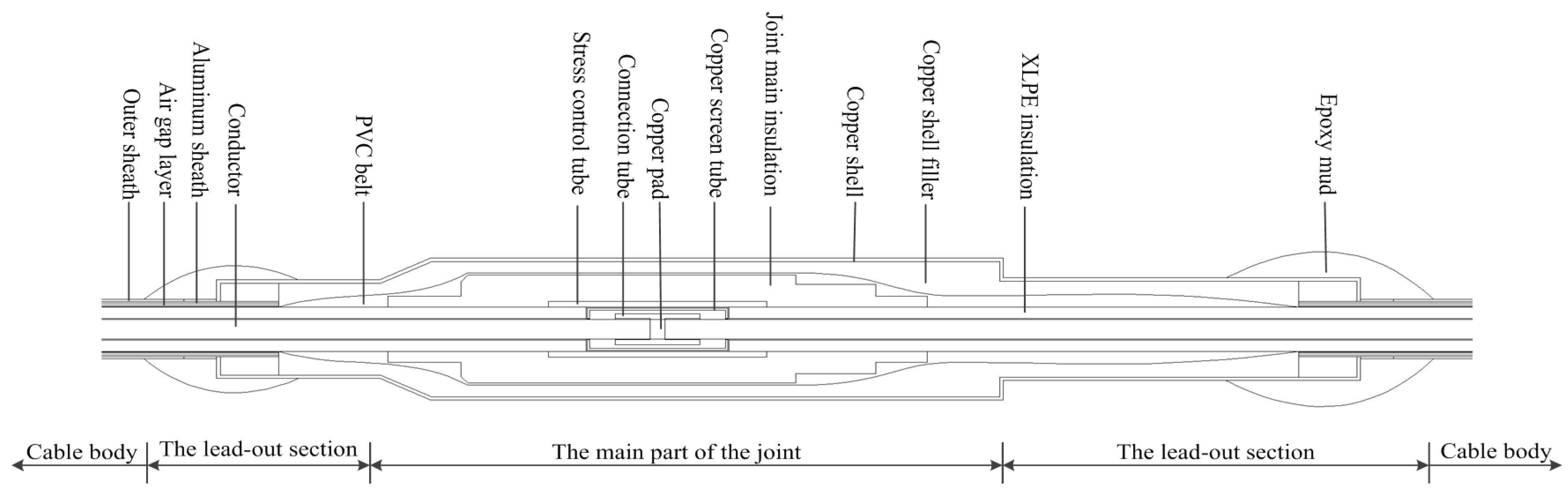
2.1. Cable Joint Geometric Model

High voltage cable normally has a single core and most of the portions of both the main body and the joint are axis symmetric. Only relatively small portions of the cable joint are asymmetric and their effects on the cable conductor’s temperature can be considered negligible [20,30]. Therefore, the cable joint can be considered as isotropic in the radial direction, and the solution for its steady-state temperature field distribution can be formulated as a 2D steady-state heat conduction problem. It has been pointed out in the literature [20] that the thermal field distribution in the cable joint as obtained by a 3D model is not necessarily more accurate than that obtained from a 2D model. Thus, this paper adopts a 2D FEA modelling approach.
The prefabricated straight-through cable joint studied in this paper is for a 110 kV 1 × 630 mm2 (single core) aluminum-sheathed, cross-linked polyethylene (XLPE) cable, which is installed in a trench. The following assumptions are made about this cable joint.
(1)
The cable has a stranded conductor and the cable joint is treated as a cylinder.
(2)
The copper protective shell is considered to be a cylindrical structure ignoring the influence of its top ground stud.
(3)
The equivalent radius is used to describe the corrugated aluminum sheath of the cable.
(4)
Small geometries, such as the earthling rod, the stress relief cone, and the shrinking belt around the copper shell, are neglected.
Figure 1 illustrates the 2D axial model of the cable joint described above. The model’s parameters are provided in Table 1. The structural parameters are obtained by actual measurement, and the thermal parameters are taken from the IEC standards.

2.2. Boundary Conditions in Modelling

The presence of the connection tube and copper pad (Figure 1) implies that the current density distribution of the conductor near the connection tube is different from that in the other parts of the cable joint. This may introduce difficulties in performing an analytical calculation of the heat generated by the conductor. Thus, the electric-thermal coupling module in finite element software ANSYS is adopted to carry out a numerical analysis to obtain the cable joint’s steady-state thermal distribution [31]. The current and voltage boundary conditions are set as:
  • One end of the cable joint’s conductor is set as the reference potential, and another end is loaded with different currents to simulate various operation conditions (as the load current is 50 Hz AC, the dielectric loss in the joint insulation is negligible).
  • The aluminium sheath is single-end grounded, so the circulation loss on the aluminium sheath is negligible.
According to IEC-60287, the equivalent resistance (consisting of contact and conductor resistance) of the cable joint is not larger than that of the cable body at the same length. Thus, the contact resistance introduced by the connection tube is ignored in the modelling.
To establish the thermal field of the cable joint in the electric-thermal coupling model, the thermal boundary conditions of the cable joint’s surface also needs to set. It can be one of the following three conditions [32]:
  • At the surface of joint, the temperature is a function of time and position (the first type of boundary condition).
  • At the surface of joint, the heat flux normal to the surface is a function of time and position (the second type of boundary condition).
  • At the surface of joint, contact with another medium can exist (the third type of boundary condition).
The operating conditions of the cable joint is complicated, and the loading current can be time varying. Thus, it is difficult to determine the temperature and heat flux at the cable joint’s boundary in real time, using either theoretical or experimental methods. The cable joint studied in this paper was under natural convection with an ambient airflow rate of less than 0.15 m/s. Thus, the cable joint is bounded by the air field. As a result, the third type of boundary condition is adopted, which assumes that the airflow temperature is the same as the ambient temperature. The natural heat transfer coefficient is decided by an empirical value, which is set as 7.5 W/m·K in this paper.
Figure 2 shows the current density distribution of the cable joint obtained from electric-thermal modelling. It can be seen that the current only flows through three components of the cable joint (the conductor, the connection tube and the copper pad), and Joule heat generated by these three components are the only heat sources in the cable joint. For the connection tube, the current is unevenly distributed and mainly near the copper pad.

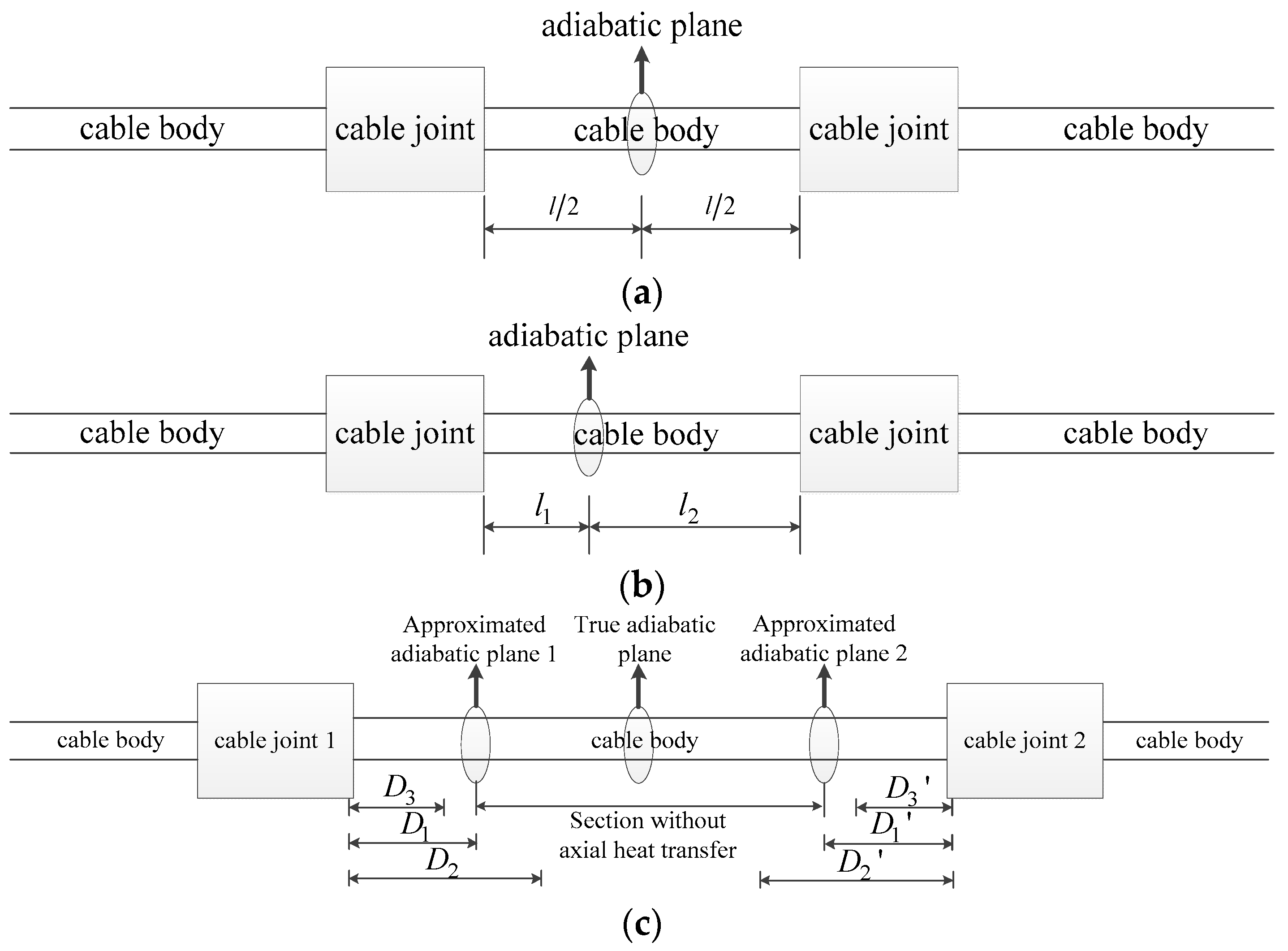
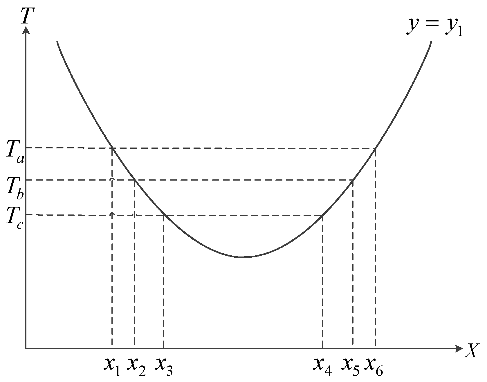
2.3. Setting the Approximated Adiabatic Plane

In an operating cable system, the length of cable body between two adjacent joints is normally between 200 and 400 m. A temperature gradient may exist between the cable joint and cable main body. The axial temperature difference leads to the presence of axial heat flow, which passes through the cable joint’s lead-out section to the cable body and gradually decays [33]. From a previous study [20], it can be inferred that the lowest temperature position of a cable is located on the cable’s main body between two adjacent joints. Thus, there is no axial heat transfer past the orthogonal plane of this position. This orthogonal plane is defined as the adiabatic plane. When the cable stretch is symmetric, the adiabatic plane between two adjacent joints is in the middle of the cable’s main body (Figure 3a). When the cable stretch is asymmetric, the adiabatic plane can be in any location along the cable’s main body (Figure 3b).
However, it might be very difficult to use a FEA method to solve the thermal distribution problem when the axial adiabatic plane is set in strict accordance with Figure 3a,b in the actual operating situation.
The cable operation experience shows that the axial temperature difference is very small at positions away from the joint. Due to the resolution of the measuring device, such small temperature differences cannot be identified. As such, the axial heat transfer influence in positions away from the joint can be neglected. In this paper, an approximated adiabatic plane for a cable joint is determined (Figure 3c).
In Figure 3c, along the extension of the lead-out section of cable joint 1 (cable joint 2), it is possible to find three planes: D1, D2 and D3 (D1′, D2′ and D3′). Their distance to cable joint 1 (cable joint 2) satisfy the relationship D2 > D1 > D3 (D2′ > D1′ > D3′), assuming the temperature at position D3 (D3′) is TD3′ (TD3’′) when D1 (D1′) is the approximated adiabatic plane while the temperature at the position D3 (D3′) is TD3″ (TD3’″) when D2 (D2′) is the approximated adiabatic plane. Then, if Δ = TD3″ − TD3′ (Δ′ = TD3’″ − TD3’′) is less than a predefined value (which can be determined through testing), the approximate adiabatic planes can be chosen at the position D1 (D1′).
The above approximated adiabatic plane is also affected by the cable’s loading condition. For the prefabricated straight-through joint studied in this paper, its ampacity cannot exceed 1600 A [9]. Thus, a 1600 A load current is used in the thermal calculation for determining the approximated adiabatic plane.
Using the above procedure, it was found that D1, D2 and D3 (D1′, D2′ and D3′) are 10, 20 and 9.5 m, respectively, for the prefabricated straight-through joint which is under investigation. This result is consistent with the instrument sensitivity, which was 0.1 °C. Therefore, two approximated adiabatic planes, one for each of the two adjacent cable joints, are set at positions 10 m away from the cable joints.

2.4. Numerical Results and Analysis

Taking into account the maximum load current that can be attained in field experiments, the cable’s load current during modelling was set at 1230 A. The steady-state thermal distribution of the cable joint is then obtained as shown in Figure 4. It can be seen that the highest temperature of the joint is at the connecting tube, while the lowest temperature is at the top of the epoxy mud. The joint’s thermal field radiates outward, elliptically centered on the connection tube. Some findings about the obtained joint’s thermal distribution at steady state are as follows. Findings 1 and 3 are consistent with those reported in the literature [19,20,21]. However, to the best knowledge of the authors, findings 2, 4 and 5 have not been reported before. These three findings may help improve the understanding of the axial thermal field and critical spot in prefabricated straight-through joints.
  • As shown in Figure 5, there is a temperature gradient along the axial direction of the cable joint’s conductor. The highest conductor temperature is at the center of the connecting tube, and reaches 91.1 °C, and the conductor temperature decreases to 69.7 °C along the axial direction away from the connecting tube. The cable joint’s structural characteristics and material thermo-physical properties cause the equivalent radial thermal resistance of the joint to be higher than that of the cable body. Therefore, the radial temperature difference inside the joint is higher than that inside the cable body under the same radial heat flow. This leads to an axial heat conduction between the joint conductor and the cable body conductor. As distance away from the connection tube increases, the effect of axial heat transfer gradually decreases, and the conductor temperature tends to be stable. From the above study, we found that the difference in surface temperatures between the cable joint and cable body is not significant (41.2 °C and 39.1 °C, respectively).
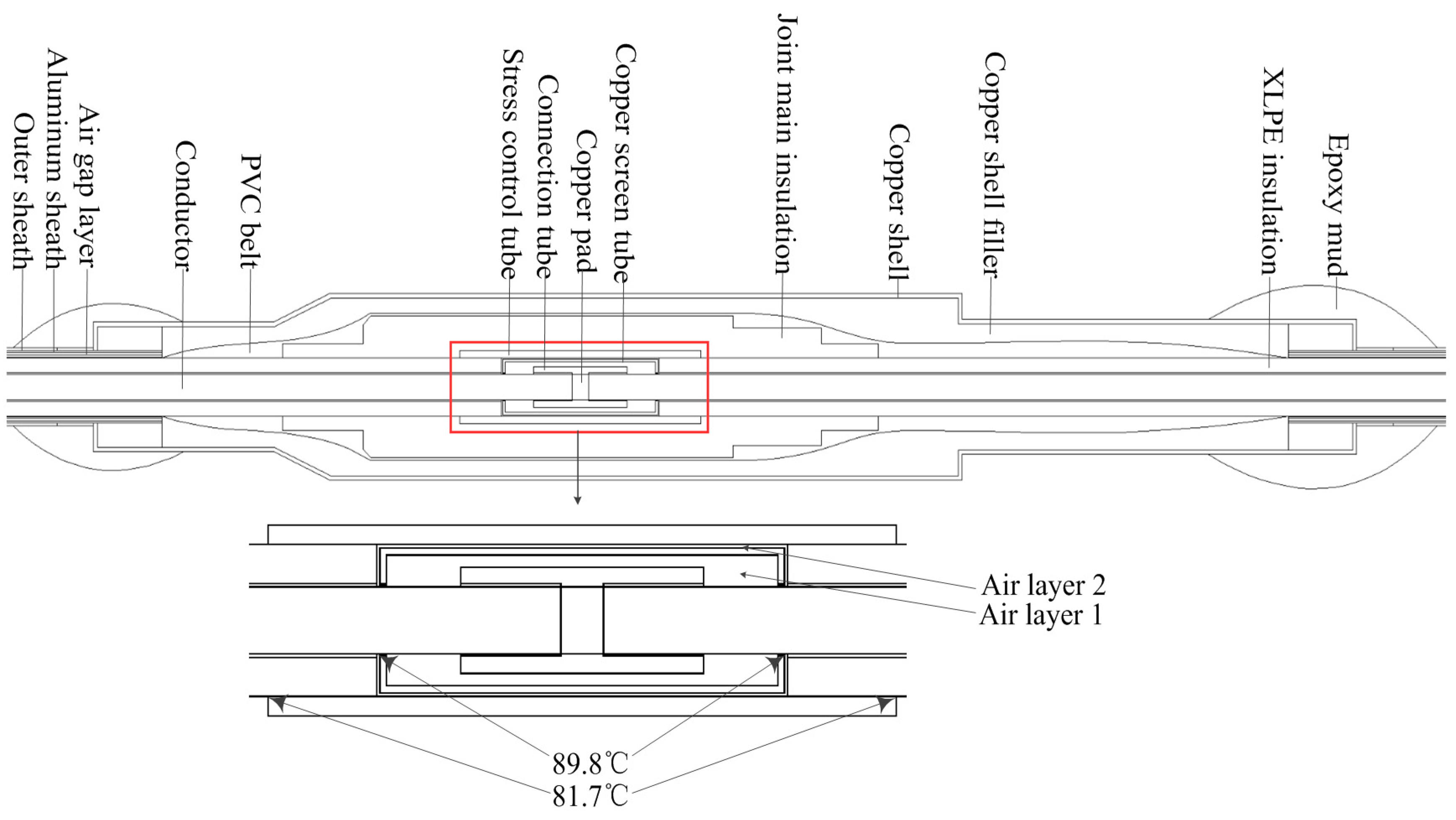
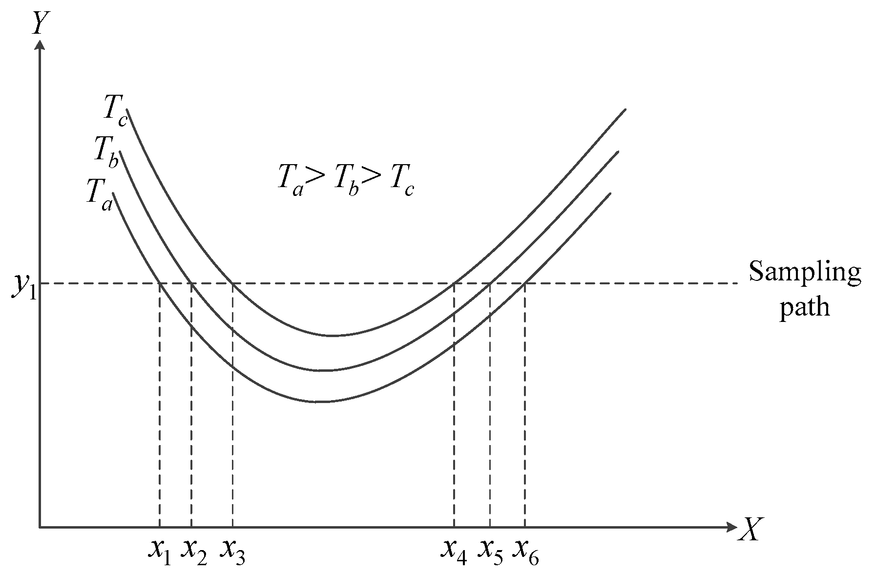
  • As is the case with the cable body, the ampacity of the cable joint is subject to the capability of the insulation to withstand long-term high temperature. Figure 6 presents the sampling result of the system shown in Figure 4. It can be seen that the insulation section of the joint adjacent to the conductor reaches 89.8 °C, which is higher than the highest temperature of the joint’s main insulation (81.7 °C). As a result, the temperature at the insulation section of the joint adjacent to the conductor becomes the critical factor limiting the ampacity of the cable joint. This section is the critical spot.
  • With the load current of 1230 A, the steady-state temperature of the conductor of the cable body is only 69.7 °C. In contrast, the highest steady-state temperature within the XLPE insulation of the joint is 89.8 °C. This temperature is almost equal to the long-term tolerance temperature (90 °C) of XLPE insulation. Therefore, the insulation of the cable joint is the critical component in determining the ampacity of a cable system.
  • As the distance away from the connecting tube increases, the cable joint’s surface temperature exhibits a slow increasing trend (from 41.2 °C to 43.5 °C) and the cable body’s surface temperature decreases to a constant value (from 43.5 °C to 39.1 °C). Thus, the highest surface temperature of the joint occurs at the end of its copper shell.
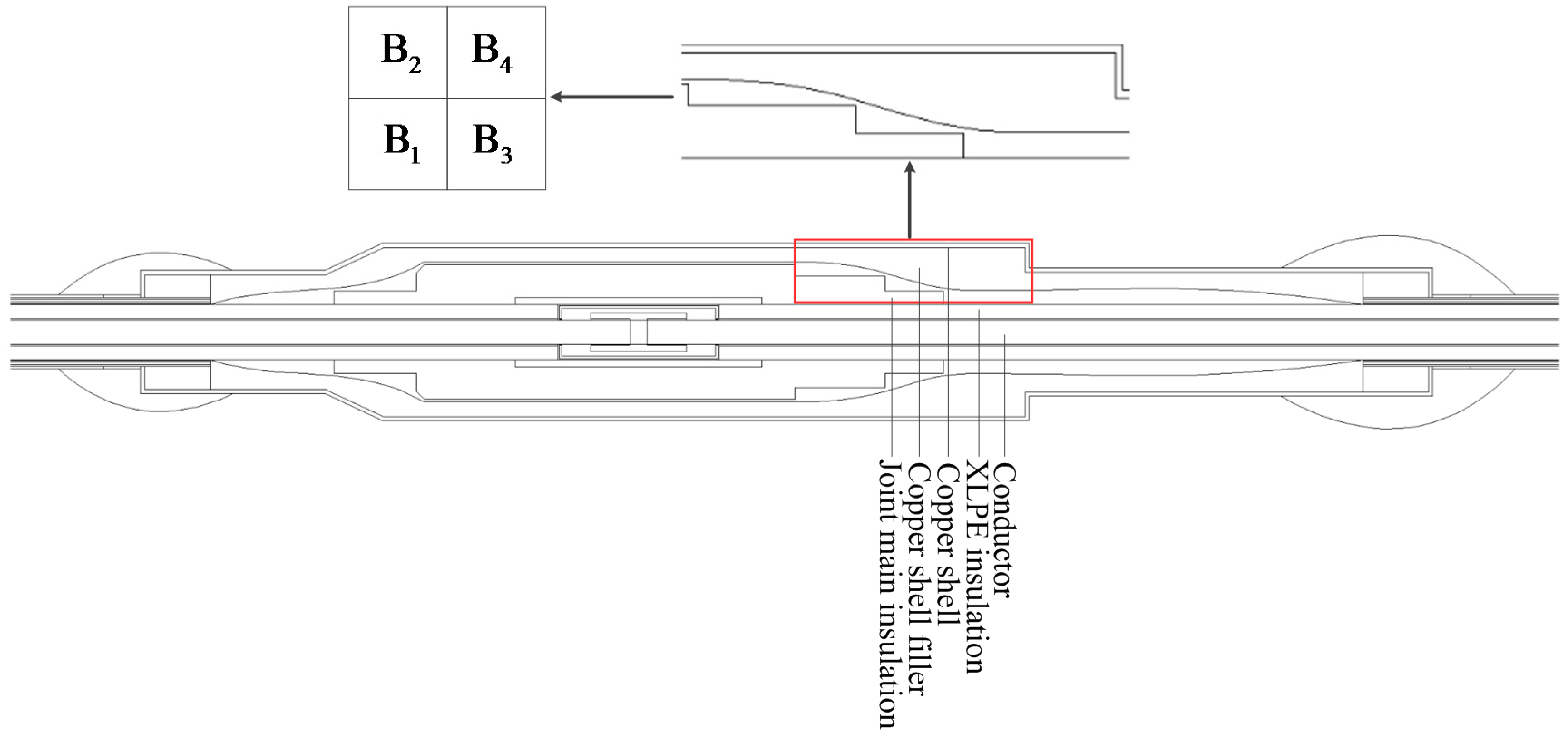
  • The modelling results reveal that the radial temperature difference inside the cable joint decreases with increasing distance away from the connecting tube. Figure 6 shows the radial thermal field distribution at the connecting tube. The temperature difference between the inner and outer diameter of each component of the connecting tube are provided in Table 2. The largest decrease in temperature in the radial direction is in the joint’s main insulation (27.9 °C) due to its thickness being the largest. Moreover, the temperature gradient in the air layer (air layer 2 in Table 2) between the copper screen tube and the stress control tube reaches 9.7 °C. This is due to the low thermal conductivity of air.
Figure 7 shows the isotherm diagram of the cable joint’s steady-state thermal field. It can be seen that the temperature near the connecting tube is higher than that of other locations away from the connecting tube. The temperature difference between the two adjacent isotherms is around 5 °C. It also can be seen from Figure 7 that some anomalous temperature regions exist. Because the steady-state thermal field of the joint is symmetrically distributed in the axial direction, only four regions (A, B, C and D) in Figure 7 are taken as examples.
In the following discussions, a normal vector is defined as pointing vertically from the high temperature isotherm toward the low temperature isotherm. Regions A and D (highlighted with circles) in Figure 7 are the insulation near the fracture of the joint’s aluminum jacket. The isotherms show a V-type trend along the normal vector of the isotherm in these two regions. The effect of the V-type isotherm can be illustrated in Figure 8 and Figure 9. In Figure 8, the X- and Y-axes represent the axial and radial displacements, respectively, of the sampling points from the geometric center of the connecting tube. Figure 9 shows the result of the sampling path along the X-axis in Figure 8; it can be seen that the temperature along the sampling path also shows the V-type trend.
The above phenomenon can be explained as follows. The temperature of the XLPE insulation layer is mainly determined by the radial heat transfer process. Near the end of the aluminum jacket, the cable body is surrounded by epoxy mud, which has a low thermal conductivity. This leads to a greater radial thermal resistance of the cable body than that of the areas A and D in the cable joint. Moreover, the joint section near the end of the aluminum jacket has a smaller radial dimension compared to the main part of the joint (Figure 1). However, the internal heat generation rate is not substantially different. Therefore, the lowest temperature appears in the XLPE insulation near the end of the aluminum jacket.
In Figure 7, regions B and C (highlighted with circles) are copper shell fillers near the end of the joint’s main insulation. The isotherms show a Λ-type trend along the normal vector of the isotherm in these two regions. This indicates that the temperature of the copper shell filler increases along the axial direction. The reason for the temperature anomaly in region B is further explained in Figure 10. In the figure, region B is further divided into four small sections B1–B4. B1 is the main insulation and B2, B3 and B4 are copper shell fillers.
The thermal conductivity of copper shell filler is twice that of the main insulation. So, the temperature difference inside the main insulation (B1) is much more significant than the temperature difference inside the copper shell fillers (B3). Moreover, the radial temperature difference between the conductor and copper shell near the end of the main insulation is not substantially different due to the high thermal conductivity of copper shell. This implies that the radial temperature difference between regions B1 and B2 is not much different than the difference between regions B3 and B4. Therefore, the radial temperature difference in region B2 is much lower than the difference in region B4. Furthermore, the difference in temperature in the axial direction of the copper shell is not obvious. Consequently, the temperature of the copper shell filler in B2 is lower than the filler in region B4.

3. Experimental Study of a Prefabricated Straight-Through Cable Joint of 110 kV XLPE Cable

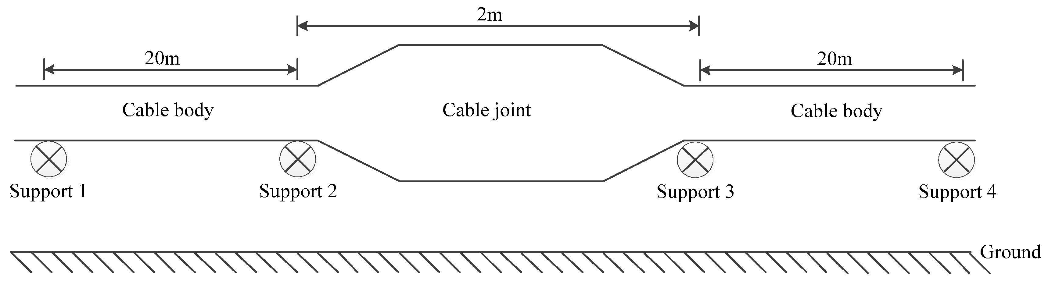
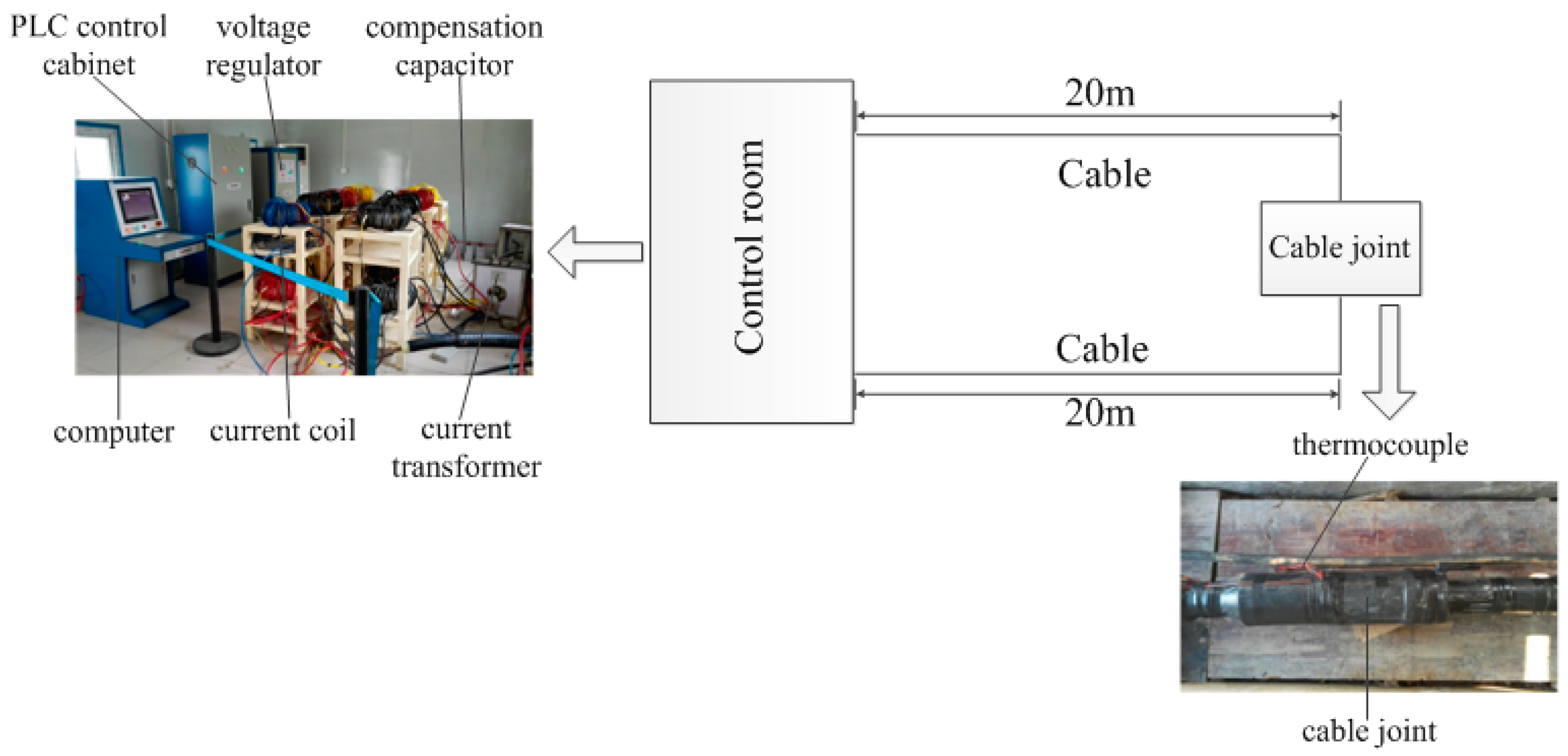
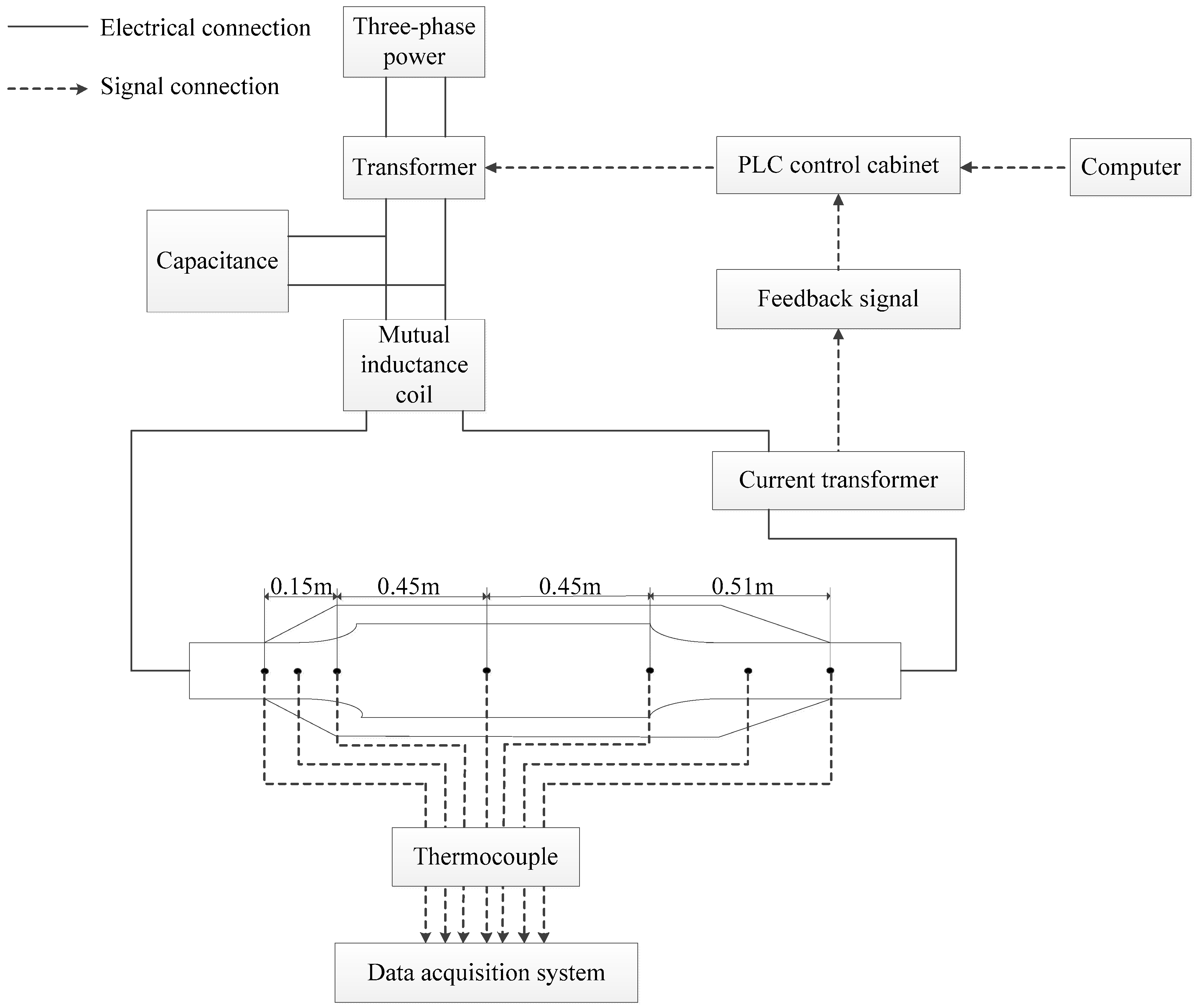
3.1. Experimental Setup

A series of steady-state temperature rise experiments were performed on a 110 kV XLPE cable with the above prefabricated straight-through cable joint. The experimental setup is shown in Figure 11, Figure 12 and Figure 13. The cable joint was put in a trench with large open ends on both sides to maintain an environment within the trench that is the same as the ambient environment. The cable either side of the joint extended for 20 m. Such a length is needed for reaching isothermal conditions. To maintain cable operation with an air laying condition, wood supports were placed under both the cable and cable joint; the surface of the cable and its joint did not touch the ground, thus avoiding heat transfer.
The structural parameters of the above cable joint have been provided in Table 1. Since the capacity of the power supply in the laboratory was not high enough, one end of the joint was grounded, i.e., the joint operated in a high-current and low-voltage mode. As shown in Figure 13, in the experiments, the current generation consisted of a three-phase power supply, a voltage regulator, a current coil and a compensation capacitor [34,35]. The feedback control comprised a computer, a programmable logic controller (PLC) control cabinet and a current transformer. The PLC adjusted the cable joint current according to the difference between the preset value and the measured value. Using this setup, the heat generated by the joint can be regulated to simulate the real operation of the cable joint.
During the experiments, temperatures were measured using thermocouples at seven measuring points along the surface of the joint’s conductor. To improve the accuracy of temperature measurement, three thermocouples were installed at each of the seven measuring points. The measured temperature was taken as the average of the readings of each of the three thermocouples. The thermocouples at the first temperature measuring point were directly attached to the surface of the crimping tube and the thermocouples at the other six measuring points were embedded into the surface of the joint’s conductor. All thermocouples were calibrated with an average measurement error of less than 0.1 °C. The thermocouples were connected to a data acquisition system for data processing and analysis.

3.2. Results and Discussion

Starting with a non-load condition, different currents were applied to the cable joint until the steady state was reached. The experiments were divided into four stages and the loads that were applied to each stage were 710, 970, 1150 and 1230 A. The measured steady state temperature of the joint’s conductor was compared with results obtained from modelling (Figure 14). It can be seen that the axial temperature distributions at different load currents obtained from the experiments agrees with those obtained from modelling.
With reference to the measured steady-state temperatures on the conductor of the cable joint, an error analysis of the modelling was conducted (Figure 15). The following observations can be made:
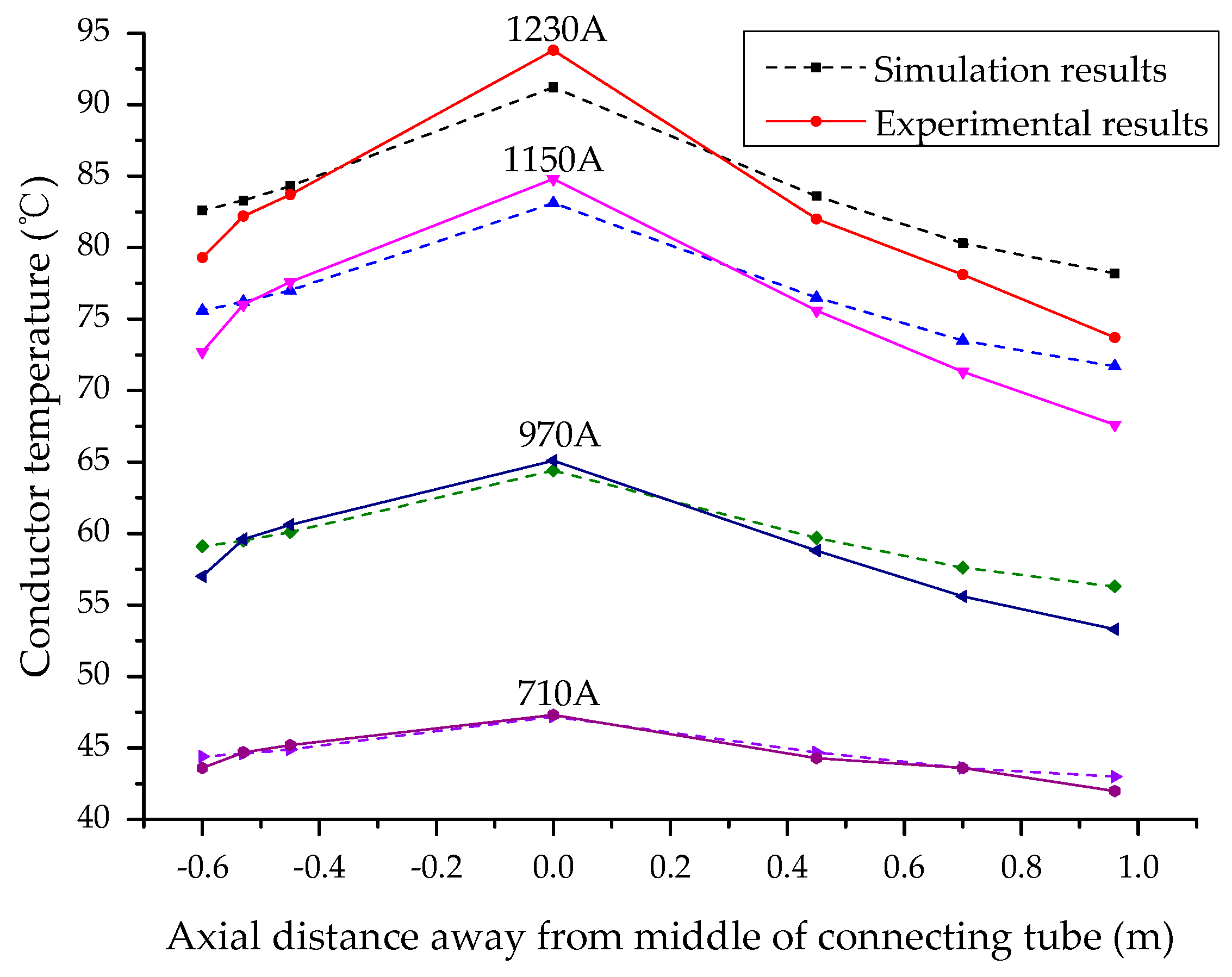
  • When applying different load currents to the joint, the maximum temperature at the steady state obtained from modelling was lower than that obtained from experiments. The discrepancies (e.g., modelling error) increased with increasing the applied load current. This might be due to the use of a connection tube in the joint, which introduces a contact resistance that may elevate the heat generation of the cable joint. The value of this contact resistance is affected by many factors and it is difficult to determine by modelling. The absence of contact resistance in the FEA modelling results in reduced heat generation of the joint; and in turn, the modelling generated lower temperature estimations compared to the experiments. With the increase of the load current, the inner temperature of the joint increases and leads to the increase of the contact resistance. This results in an increase in modelling error.
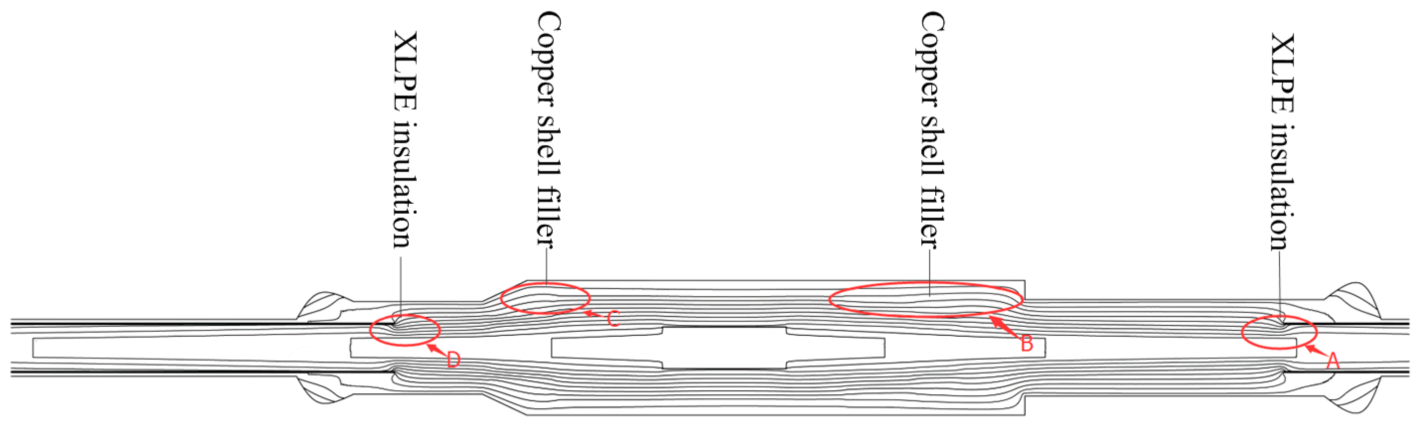
  • Under different load currents, the largest modelling error of the steady state conductor temperature is in the copper shell port on the longer half of the joint. Due to the imperfection of the installation process, the aluminum sheath and the copper shell may not tightly overlap in the cable joint and a void may exist between them. The influence of the void was not considered in the modelling. On the other hand, the epoxy mud used to seal the end of the copper shell in the experiments was manually applied. As such, the real shape of the mud cannot be exactly described in modelling.
  • The absolute error in the FEA modelling of the steady-state conductor temperature was less than 7% with reference to the experimental results. Thus, the model results are sufficiently accurate to be practically applied.
Therefore, it can be concluded that the accuracy of the joint electric-thermal modelling approach developed in this paper can provide reliable temperature estimation for the purposes of calculating the ampacity of a cable joint. The next section presents an algorithm that estimates the cable joint’s ampacity based on the findings of both the modelling and experiments.

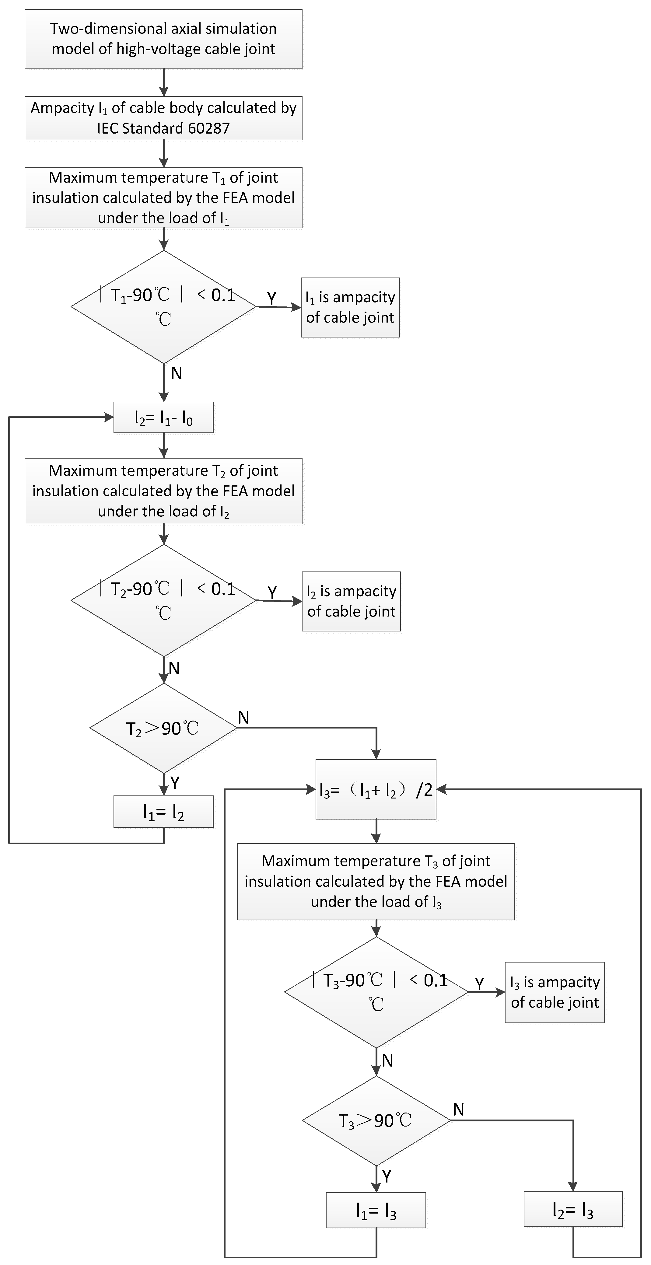
4. Ampacity Calculation of the Cable Joint

The accurate evaluation of a cable joint’s ampacity is very important for on-line cable condition monitoring [36,37]. In this paper, an algorithm has been developed for estimating the cable joint’s ampacity based on the theoretical and experimental results as presented in Section 2 and Section 3.
The algorithm adopts an iterative approach and uses the XLPE insulation’s long-term tolerance temperature as the criterion. The algorithm can eventually approach the highest tolerance current, i.e., the cable joint’s ampacity. The iterative process is considered to have converged when the temperature difference between the model estimate and the XLPE insulation’s long-term tolerance temperature is within a pre-defined limit. In this algorithm, the iteration constant (i.e., I0) is set to 100 A. The ampacity of the cable main body, as calculated by International Electrotechnical Commission (IEC) Standard 60287 (i.e., I1), is set as the initial value of the iteration. The whole procedure of the algorithm is shown in Figure 16. In Figure 16, I2 and I3 are the intermediate variables generated in the iteration.
Using the procedure shown in Figure 16, the ampacity of a cable joint under different loading and weather conditions (natural convection and temperature) can be calculated as shown in Figure 17 and Figure 18. With some modifications, the algorithm can also be used for the calculation of a cable body’s ampacity. To further prove that the joint is one of the hot spots in the whole cable system, we take the case when the ambient temperature is 25 °C and the natural heat transfer coefficient is 7.5 W/m·K as an example. The calculated results show that the ampacity of the cable joint is 1255 A, which is 19% lower than the ampacity of the cable body (1556 A). This verifies that the ampacity of a cable joint under the same environmental conditions is lower than the ampacity of cable body with the same conductor cross section.
Figure 17 shows the relationship between the ambient temperature and the cable joint’s ampacity under different convection heat transfer coefficients. It can be seen that the ampacity of a joint tends to linearly increase with the ambient temperature. This phenomenon can be explained by heat transfer theory. When the ambient temperature changes within a certain range, its influence on heat production and the material thermal conductivity can be neglected. Therefore, the temperature difference between the joint conductor and the ambient environment is almost constant, regardless of the change in ambient temperature.
Figure 18 shows the relationship between the convection heat transfer coefficient and the joint’s ampacity under different ambient temperatures. It can be seen that the ampacity of a joint tends to rise with an increase in the convection heat transfer coefficient; however, the changing rate gradually decreases. This is because increasing the convection heat transfer coefficient can promote heat transfer between the joint surface and the ambient environment. Thus, the temperature difference between the cable joint’s conductor and the ambient environment decreases with an increase in the convection heat transfer coefficient.

5. Conclusions

  • This paper developed an electric-thermal coupling model for a prefabricated straight-through joint of a 110 kV cable system. The model was successfully applied to obtain the joint’s steady-state thermal distribution and to evaluate the joint’s ampacity.
  • Based on the joint’s steady-state thermal distribution, as obtained by this model, it was pointed out that the XLPE insulation section of the joint adjacent to the conductor became the critical spot limiting the ampacity of the joint.
  • Based on the algorithm presented in Section 4, it was found that the ampacity of a cable joint is much lower than the ampacity of its cable body.
  • Comprehensive experiments on a real cable system with a prefabricated straight-through joint under different loading conditions were conducted. The experimental results verified that the model developed in this paper can be used for determining the ampacity of prefabricated straight-through joints of high voltage cable.

Acknowledgments

This project is supported by the National Natural Science Foundation of China (No. 51477054). The authors gratefully acknowledge the Cable Specialty Committee of the Guangdong Society for Electrical Engineering for providing technical assistance and the Transmission Management of Guangzhou Power Supply Bureau Ltd. for providing experimental locations. The authors would like to thank the anonymous reviewers for their instructive comments.

Author Contributions

This paper is a result of the collaboration of all co-authors. Gang Liu conceived and designed the study. Pengyu Wang established the thermal model and wrote the paper. Hui Ma helped with most of the corrections. Yigang Liu designed all the experiments. Tao Xu performed the experiments.

Conflicts of Interest

The authors declare no conflict of interest.

References

  1. Li, H.J.; Tan, K.C.; Su, Q. Assessment of underground cable ratings based on distributed temperature sensing. IEEE Trans. Power Deliv. 2006, 21, 1763–1769. [Google Scholar] [CrossRef]
  2. Huang, R.; Pilgrim, J.A.; Lewin, P.L.; Payne, D. Dynamic cable ratings for smarter grids. In Proceedings of the 4th IEEE PES Innovative Smart Grid Technologies Europe, Copenhagen, Denmark, 6–9 October 2013; pp. 1–5. [Google Scholar] [CrossRef]
  3. Marc, D.A.; Francisco, L. Adaptive soil model for real-time thermal rating of underground power cables. IET Sci. Meas. Technol. 2014, 9, 654–660. [Google Scholar] [CrossRef]
  4. Li, Y.; Wouters, P.A.A.F.; Wagenaars, P.; Wielen, P.C.J.M.; Steennis, E.F. Temperature dependent signal propagation velocity: Possible indicator for MV cable dynamic rating. IEEE Trans. Dielectr. Electr. Insul. 2015, 22, 665–672. [Google Scholar] [CrossRef]
  5. Sujit, P.; Francisco, L.; Matthew, T. Calculation of cable thermal rating considering non-isothermal earth surface. IET Gener. Transm. Distrib. 2014, 8, 1354–1361. [Google Scholar] [CrossRef]
  6. Neher, J.H.; McGrath, M.H. The calculation of the temperature rise and load capability of cable systems. AIEE Trans. 1957, 76, 752–772. [Google Scholar] [CrossRef]
  7. Anders, G.J. Rating of Electrical Power Cable, 1st ed.; IEEE Press: New York, NY, USA, 1997. [Google Scholar]
  8. Anders, G.J. Rating of Electric Power Cables in Unfavourable Thermal Environment, 1st ed.; IEEE Press: Piscataway, NJ, USA, 2005. [Google Scholar]
  9. International Electrotechnical Commission. Calculation of the Current Rating of Electric Cables; IEC 60287; IEC Press: Geneva, Switzerland, 2006. [Google Scholar]
  10. Insulated Conductors Committee of the IEEE Power Engineering Society. IEEE GUIDE for Soil Thermal Resistivity Measurements; IEEE Std 442, reaffirmed 2003; IEEE: Piscataway, NJ, USA, 1981. [Google Scholar]
  11. Frank, D.W.; Jos, V.R.; George, A.; Bruno, B.; Rusty, B.; James, P.; Marcio, C.; Georg, H. A Guide for Rating Calculations of Insulated Cables; Cigré TB # 640; Cigré: Paris, France, 2015. [Google Scholar]
  12. International Council on Large Electricsystems. Cable Rating Verification; Cigré WG B1.56; Cigré: Paris, France, 2016. [Google Scholar]
  13. Benato, R.; Colla, L.; Dambone Sessa, S.; Marelli, M. Review of high current rating insulated cable solutions. Electr. Power Syst. Res. 2016, 133, 36–41. [Google Scholar] [CrossRef]
  14. Eric, D.; Laurent, M.; Udo, F.; Vince, B.; Christian, R.; Jose, M.M.; Asakiyo, U.; Graeme, B.; Mike, S. Large Cross-Sections and Composite Screens Design; Cigré Technical Brochure 272 by WG B1.03; Cigré: Paris, France, 2005. [Google Scholar]
  15. Benato, R.; Paolucci, A. Multiconductor cell analysis of skin effect in Milliken type cables. Electr. Power Syst. Res. 2012, 90, 99–106. [Google Scholar] [CrossRef]
  16. Villacci, D.; Vaccaro, A. Transient tolerance analysis of power cables thermal dynamic by interval mathematic. Electr. Power Syst. Res. 2007, 77, 308–314. [Google Scholar] [CrossRef]
  17. Luoni, G.; Morello, A.S.; Crockett, A.E. Continuous current rating for external and surface cooled cable systems. IEE Proc. C 1981, 128, 129–139. [Google Scholar] [CrossRef]
  18. Belli, S.; Perego, G.; Bareggi, A.; Caimi, L.; Donazzi, F.; Zaccone, E. P-Laser: Breakthrough in power cable systems. In Proceedings of the 2010 IEEE International Symposium Electrical Insulation(ISEI), San Diego, CA, USA, 6–9 June 2010. [Google Scholar] [CrossRef]
  19. Yang, F.; Cheng, P.; Luo, H.; Yang, Y.; Liu, H.; Kang, K. 3-D thermal analysis and contact resistance evaluation of power cable joint. Appl. Therm. Eng. 2015, 93, 1183–1192. [Google Scholar] [CrossRef]
  20. Pilgrim, J.A.; Swaffield, D.J.; Lewin, P.L.; Payne, D. An investigation of thermal ratings for high voltage cable joints through the use of 2D and 3D Finite Element Analysis. In Proceedings of the 2008 IEEE International Symposium on Electrical Insulation, Vancouver, BC, Canada, 9–12 June 2008; pp. 534–546. [Google Scholar] [CrossRef]
  21. Pilgrim, J.A.; Swaffield, D.J.; Lewin, P.L.; Payne, D. Assessment of the impact of joint bays on the ampacity of high-voltage cable circuits. IEEE Trans. Power Deliv. 2009, 24, 1029–1036. [Google Scholar] [CrossRef]
  22. Nakamura, S.; Morooka, S.; Kawaski, K. Conductor temperature monitoring system in underground power transmission XLPE cable joints. IEEE Trans. Power Deliv. 1992, 7, 1688–1697. [Google Scholar] [CrossRef]
  23. Abdel Aziz, M.M.; Riege, H. A new method for cable joints thermal analysis. IEEE Trans. Power Appar. Syst. 1980, 99, 2386–2392. [Google Scholar] [CrossRef]
  24. Chang, H.; Tan, T.; Ruan, J.; Gao, Y.; Liu, K. Research on temperature retrieval and fault diagnosis of the cable joint. In Proceedings of the 39th Annual Conference of the IEEE Industrial Electronics Society (IECON2013), Vienna, Austria, 10–13 November 2013; pp. 7388–7393. [Google Scholar] [CrossRef]
  25. Ruan, J.; Liu, C.; Huang, D.; Zhan, Q.; Tang, L. Hot spot temperature inversion for the single-core power cable joint. Appl. Therm. Eng. 2016, 104, 146–152. [Google Scholar] [CrossRef]
  26. Hwang, C.C.; Chang, J.J.; Chen, H.Y. Calculation of ampacities for cables in trays using finite elements. Electr. Power Syst. Res. 1999, 54, 75–81. [Google Scholar] [CrossRef]
  27. Lin, S.; Hu, W. Theoretical research on temperature field of power cable joint with FEM. In Proceedings of the International Conference on System Science and Engineering (ICSSE), Dalian, China, 30 June–2 July 2012; pp. 564–567. [Google Scholar] [CrossRef]
  28. Fu, J.; Cheng, P.; Chen, W.; Yang, Q.; Hu, X.; Wang, Q.; Yang, F. Investigation of the effects of insulation defects on the 3-D electromagnetic-thermal coupling fields of power cable joint. In Proceedings of the 2016 IEEE 11th Conference on Industrial Electronics and Applications (ICIEA), Hefei, China, 5–7 June 2016; pp. 1436–1439. [Google Scholar] [CrossRef]
  29. Yang, F.; Liu, K.; Cheng, P.; Wang, S.; Wang, X.; Gao, B.; Fan, Y.; Xia, R.; Ullah, I. The coupling fields characteristics of cable joints and application in the evaluation of crimping process defects. Energies 2016, 9, 932. [Google Scholar] [CrossRef]
  30. Illias, H.A.; Lee, Z.H.; Bakar, A.H.A.; Mokhlis, H.; Chen, G.; Lewin, P.L. Electric field distribution in 132 kV one piece premolded cable joint structures. In Proceedings of the IEEE International Conference of Condition Monitoring and Diagnosis, Bail, Indonesia, 23–27 September 2012; pp. 643–646. [Google Scholar] [CrossRef]
  31. Rachek, M.; Larbi, S.N. Magnetic eddy-current and thermal coupled models for the finite-element behaviour analysis of underground power cables. IEEE Trans. Magn. 2008, 4, 4739–4746. [Google Scholar] [CrossRef]
  32. Baehr, H.D.; Stephan, K. Heat conduction and mass diffusion. In Heat and Mass Transfer, 2nd ed.; Springer: Berlin, Germany, 2006; pp. 111–114. [Google Scholar]
  33. Liu, G.; Lei, M.; Ruan, B.; Zhou, F.; Li, Y.; Liu, Y. Model research of real-time calculation for single-core cable temperature considering axial heat transfer. High Volt. Eng. 2012, 38, 1877–1883. [Google Scholar] [CrossRef]
  34. Liu, G.; Lei, C. Experimental analysis on increasing temporary ampacity of single-core cable. High Volt. Eng. 2011, 37, 1288–1293. [Google Scholar] [CrossRef]
  35. Lei, C.; Liu, G.; Ruan, B.; Liu, Y. Experimental research of dynamic capacity based on conductor temperature-rise characteristic of HV single-core cable. High Volt. Eng. 2012, 38, 1397–1402. [Google Scholar] [CrossRef]
  36. Aras, F.; Oysu, C.; Yilmaz, G. An assessment of the methods for calculating ampacity of underground power cables. Electr. Power Compon. Syst. 2005, 33, 1385–1402. [Google Scholar] [CrossRef]
  37. Swaffield, D.J.; Lewin, P.L.; Sutton, S.J. Methods for rating directly buried high voltage cable circuits. IET Gener. Transm. Distrib. 2007, 2, 393–401. [Google Scholar] [CrossRef]
Figure 1. 2D axial model of the 110 kV prefabricated straight-through cable joint.
Energies 10 02050 g001
Figure 2. Current density distribution of the cable joint.
Energies 10 02050 g002
Figure 3. Adiabatic plane of the cable joint: (a) adiabatic plane with symmetrical cable stretch, (b) adiabatic plane with asymmetrical cable stretch and (c) illustration of the method for setting the approximated adiabatic plane.
Energies 10 02050 g003
Figure 4. Steady-state thermal field distribution of the cable joint.
Energies 10 02050 g004
Figure 5. Conductor temperature distribution of the cable joint and nearby cable body (the axis origin is the geometric center of the connecting tube in the cable joint).
Energies 10 02050 g005
Figure 6. The sampling result of Figure 4.
Energies 10 02050 g006
Figure 7. Isotherm distribution of steady-state temperature field in the cable joint.
Energies 10 02050 g007
Figure 8. Partially enlarged V-type isotherms in the cable joint.
Energies 10 02050 g008
Figure 9. Sampling results along the axial direction in Figure 7.
Energies 10 02050 g009
Figure 10. Partially enlarged region B in Figure 7.
Energies 10 02050 g010
Figure 11. Cable installation diagram.
Energies 10 02050 g011
Figure 12. Experimental system.
Energies 10 02050 g012
Figure 13. Schematic diagram of the experimental setup.
Energies 10 02050 g013
Figure 14. Comparisons between experimental and modelling results under different loads.
Energies 10 02050 g014
Figure 15. Modelling error analysis.
Energies 10 02050 g015
Figure 16. Algorithm for calculating cable joint ampacity. FEA denotes finite element analysis.
Energies 10 02050 g016
Figure 17. Cable joint ampacity under different ambient temperatures.
Energies 10 02050 g017
Figure 18. Cable joint ampacity for different convection heat transfer coefficients.
Energies 10 02050 g018
Table 1. Detailed information of the prefabricated straight-through joint.
ComponentMaterialThickness (mm)Thermal Conductivity (W·m−1·K−1)
ConductorCopper15.0401
Connection tubeCopper7.3401
Conductor ShieldPolyolefin1.50.38
Insulation ShieldPolyolefin1.00.38
XLPE InsulationCross-linked Polyethylene17.00.4
Joint Main InsulationEthylene Propylene Rubber/0.25
PVC BeltPolyvinyl Chloride2.00.1667
Copper Shell FillerEpoxy Resin Sealant/0.5
Copper ShellCopper3.1401
Air Gap LayerAir3.00.023
Aluminum SheathAluminum2.5237
Outer SheathMedium Density Polyethylene3.00.32
Table 2. Radial temperature differences of each component at the position of the connecting tube in the cable joint.
The StructureInner Diameter Temperature (°C)Outer Diameter Temperature (°C)Temperature Difference (°C)
Conductor91.191.00.1
Air layer 191.089.81.2
Copper screen tube89.889.80
Air layer 289.880.19.7
Stress control tube80.174.45.7
Main Insulation74.447.427.0
Copper Shell Filler47.441.36.1
Copper Shell41.341.20.1
Air layer 1—the air layer between the connecting tube and the copper screen tube; Air layer 2—the air layer between the copper screen tube and the stress control tube.

